Understanding block rotation along strike-slip fault zones in Yunnan (China): paleomagnetic and structural approach.

Dottorato di ricerca in Scienze Geologiche, Biologiche e Ambientali

UNDERSTANDING BLOCK ROTATION ALONG

STRIKE-SLIP FAULT ZONES IN YUNNAN (CHINA):

PALEOMAGNETIC AND STRUCTURAL APPROACH

Ph.D Thesis

Dott.ssa Alessandra Giovanna Pellegrino

Coordinatore dottorato : Relatore/Correlatore :

Prof. Agata Di Stefano Prof. Rosanna Maniscalco

Prof. Fabio Speranza

XXXI CICLO

2015/2018

3 Introduzione e scopo del Progetto di Ricerca

Durante gli ultimi decenni, sono stati proposti diversi modelli tettonici per spiegare la deformazione e le rotazioni di blocchi crostali, attorno ad assi verticali, in zone di taglio o strike-slip. Un metodo per validare questi modelli è l’analisi paleomagnetico - strutturale realizzata proprio lungo le più importanti faglie trascorrenti del mondo.

L'area di studio proposta per il progetto di ricerca di questo dottorato, è stata analizzata da un classico e noto lavoro di Tapponnier et alii [1982], che descrive, attraverso un modello analogico con la plastilina, l’indentazione della placca Indiana nel continente Euro-Asiatico. Ciò avrebbe prodotto, a partire da 40-50 Ma, età della collisione tra i continenti India ed Eurasia, ispessimento crostale nell’area a nord e nord-est della catena Himalayana e l’estrusione del blocco Indocinese verso sud-est. Uno dei principali punti d’interesse sulla deformazione continentale e sull'evoluzione tettonica dell'Asia [Molnar, 1988], ed ancora oggetto di acceso dibattito, è il ruolo delle grandi faglie strike-slip che, probabilmente, hanno guidato l’estrusione del blocco Indocinese.

Un primo gruppo di studiosi considera la crosta essenzialmente rigida, con la deformazione concentrata lungo i suoi margini: in questo modello, le faglie trascorrenti litosferiche hanno grandi rigetti ed grandi tassi di movimento. Un secondo gruppo lega la deformazione della crosta continentale ispessita, come quella Tibetana, allo scollamento ed alla deformazione omogenea di un sottile settore crostale, a comportamento viscoso, soggetto a rotazioni e raccorciamento. Gran parte di questa controversia è focalizzata proprio sul ruolo e sul rigetto orizzontale della faglia del Red River, lunga circa 1000 km e che si estende con orientazione NW-SE dall’angolo SE del Tibet fino al Mar Cinese Meridionale. Questa faglia, insieme alla Gaoligong e alla Chongshan, dividono strutturalmente la provincia dello Yunnan (Cina sud-occidentale) in tre blocchi crostali più piccoli caratterizzati da un’intensa attività sismica. In questa tesi, si propone pertanto uno studio paleomagnetico e strutturale lungo queste faglie, al fine di valutare se, e con quale entità, queste siano responsabili della deformazione e delle rotazioni dei blocchi crostali che compongono la regione dello Yunnan.

4 Riassunto

I dati raccolti durante i tre anni di attività di Dottorato di Ricerca riguardano il paleomagnetismo di rocce sedimentarie e vulcaniche affioranti lungo due importanti zone di taglio che caratterizzano la provincia dello Yunnan (Cina): la faglia Gaoligong e la faglia del Red River. Durante il primo anno, sono stati campionati 50 siti (per un totale di 503 campioni) a distanze variabili (fino a ~25 km) dalle miloniti affioranti lungo la zona di taglio Gaoligong. I red beds di età Giurassico-Cretaceo, registrano rotazioni orarie rispetto al blocco Euro-Asiatico, che raggiungono il picco massimo (176°) in prossimità della faglia e diminuiscono progressivamente spostandosi verso est. Ad ovest della faglia Gaoligong invece, i siti di età Pliocene-Olocene, affioranti nel campo vulcanico di Tengchong, non evidenziano significative rotazioni. Pertanto, i dati dimostrano che l'attività della zona di taglio Gaoligong ha prodotto rotazioni orarie significative probabilmente coeve ai principali movimenti tettonici avvenuti nell’Eocene-Miocene. Il modello di rotazione dei blocchi crostali lungo la zona di taglio Gaoligong, risponde ad un modello cinematico crostale “quasi - continuo”, con blocchi di dimensioni ≤1 km vicino alla faglia, la cui dimensione aumenta allontanandosi verso est. I valori di rotazione e di dimensione della zona di deformazione, si traducono in un rigetto orizzontale della faglia Gaoligong di circa 230-290 km.

Al fine di investigare ulteriormente il ruolo delle faglie nella cinematica dello Yunnan, durante il secondo anno di dottorato, sono stati campionati altri 44 siti di età Triassico -Cretaceo (per un totale di 425 campioni) su entrambi i lati della zona di taglio del Red River e all’interno dei blocchi Chuandian, Lanping e Simao settentrionale. Quasi tutti i siti hanno prodotto componenti di magnetizzazione misurabili e stabili, ma la cronologia di acquisizione della magnetizzazione appare diversa nei tre blocchi. I dati evidenziano una rotazione variabile e differenziale che, anche in questo caso, non supporta un modello di rotazione rigida dei blocchi come proposto da autori precedenti, ma piuttosto suggerisce che: 1) il blocco Simao è costituito da blocchi minori (pochi km) che ruotano in senso orario, separati

5

da domini non rotanti di dimensioni simili; 2) una componente di magnetizzazione di alta temperatura (640-680 °C) suggerisce un comportamento rotazionale simile (blocchi secondari con rotazione oraria, antioraria e non-ruotati), anche al centro del “blocco” Lanping; al contrario, una componente di media temperatura (300-640 °C) acquisita successivamente al 28% della fase di piegamento non ha registrato alcuna rotazione. I siti vicini (entro i 25 km) al sistema di faglie della Red River, localizzati nel “blocco” Lanping producono invece grandi rotazioni dell'ordine di 180°. Anche i siti localizzati a 10-15 km di distanza dalla zona di taglio Chongshan mostrano rotazioni antiorarie di circa 90°, in accordo con il movimento sinistro della faglia.

I dati del presente lavoro, per la prima volta mostrano che le tre faglie Gaoligong, Chongshan e Red River influenzano significativamente le rotazioni di piccoli blocchi crostali nelle immediate vicinanze delle grandi faglie trascorrenti. Tuttavia, il verificarsi di ulteriori rotazioni (dell’ordine di 20°) all’interno dei blocchi Baoshan e Lanping - Simao, a distanze di oltre 20 km dalle faglie, lascia ancora aperto il quadro della deformazione e delle rotazioni di blocchi crostali che caratterizzano la provincia dello Yunnan.

6 Abstract

Data from this study report on the paleomagnetism of sedimentary and volcanic rocks cropping out near the Gaoligong and Ailao-Shan Red River Shear Zones. Fifty paleomagnetic sites were analyzed collecting 503 samples, during the first year of Ph.D., at variable distances (up to ~25 km) from mylonites exposed along the Gaoligong fault. Jurassic-Cretaceous red bed sites yield systematic CW rotations with respect to Eurasia reaching the peak values of 176° close to the fault, and progressively decrease moving eastward, up to be virtually annulled ~20 km E of mylonite contact. West of the Gaoligong fault, Pliocene-Holocene sites from the Tengchong volcanic field do not rotate. Thus, data show that the Gaoligong Shear Zone activity yielded significant CW rotations that were likely coeval to the main Eocene-Miocene episodes of dextral fault shear. The Gaoligong zone rotation pattern conforms to a quasi-continuous crust kinematic model, and shows blocks of ≤1 km size close to the fault, which become bigger moving eastward. Rotation and width values of the rotated-deformed zone translate to a 230-290 km Gaoligong Shear Zone dextral offset, which shows that fault shear plays a significant role in Indochina CW block rotation.

During the second year of Ph.D., forty-four Triassic-Cretaceous sites (425 samples) were collected at both sides of the Ailao-Shan Red River Shear Zone (ARRSZ), within the Chuandian, Lanping and Northern Simao blocks. Nearly all sites yielded measurable and stable magnetization components, but magnetization acquisition timing was different in the three blocks. Sites from the Chuandian block show a normal polarity and were remagnetized after folding. In the northern Simao block the magnetization was acquired before folding (about 33 Ma ago), but the ubiquitous normal polarity in Jurassic-Cretaceous sites suggests a pre-folding magnetic overprint. The data show variable and different rotation that do not display evidence of a rigid block rotation, but suggest that the northern Simao block is made of small (few km size) sub-blocks rotating CW, separated by non-rotating domains of similar

7

size. Finally, a high-temperature (640-680°C) magnetization component suggests a similar rotational behaviour (CW-rotating and non-rotating sub-blocks) in the centre of the Lanping block. Conversely, a 300-640°C component was later acquired at 28% unfolding and subsequently underwent no rotation. The sites close (less than 25 km) to the ARRSZ yield great rotations of nearly 180°, which confirm past occurrence of significant strike-slip shear along the ARRSZ itself. Conversely, sites located at 10-15 km distance from the Chongshan Shear Zone show ca. 90° CCW rotations that imply a left-lateral shear along the fault zone, consistently with recent geological evidence. Summarizing, data from my Ph.D. study, together with previous evidence of rotations documented both near the fault zones and within the blocks themselves, show that crustal deformation of the Yunnan is extremely complex and still puzzling. The Baoshan and Lanping-Simao blocks underwent strong internal deformation and were likely fragmented in smaller independent sub-blocks whose kinematics and tectonics are still a matter of speculation.

8 Guide of this thesis

This research is divided into four parts.

Part I contains six chapters. A brief introduction to the aim of the research presented in this thesis. Chapter 1, shows the state-of-the-art of the kinematic models of block rotation, fundamental setting to this research. The second and third Chapter include a brief overview of

the matter of Paleomagnetism and the methods used for gathering paleomagnetic directions through in situ sampling and paleomagnetic analysis in laboratory. Chapter 4 and 5 regard the

geological setting of the studied area and the description of paleomagnetic data collected by the previous authors in adjacent areas.

Part II, reports the outcomes from the research along the Gaoligong Shear Zone in Yunnan (Chapter 6), recently published on Tectonics by Pellegrino et al. [2018].

Part III, includes the results of the paleomagnetic analysis of the rotation pattern along the Ailaoshan Red River Shear Zone (Chapter 7), and of the deformation inside the Lanping,

Simao and Chuandian blocks. The use of anisotropy of magnetic susceptibility (AMS) measurements (Chapter 8) and magnetic mineralogy analysis (Chapter 9) permit to infer

tectonic deformation.

Finally, in Part IV there are the concluding remarks of this research (Chapter 10), followed

9

Introduction

Previous paleomagnetic data from Yunnan (China) showed a predominant post-Cretaceous clockwise (CW) rotation pattern, mostly explained invoking huge (hundreds of km wide) blocks, laterally escaping (and/or rotating) due to India-Asia collision, separated by major strike-slip shear zones. However, the matter of crustal blocks rotation pattern inside the deforming zone of strike-slip faults, remains still highly controversial. Two set of models

have been proposed to explain the rotation of Indochina block: afirst set of models suggests

that CW rotations of Yunnan are the result of lateral escape of Tibet that rotated CW around the north-eastern corner of the Indian Plate called “Eastern Himalayan syntaxis” [e.g. Chen et al., 1995; Funahara et al., 1992, 1993; Kondo et al., 2012; Sato et al., 2001, 2007; Tanaka et al., 2008; Tong et al., 2013]. However, this may explain CW rotations of the northern part of Indochina, but can hardly account for the CW rotations documented further south, at 21°-22°N latitudes.

A second set of models [Gao et al., 2015; Wang et al., 2008; Zhao et al., 2015] argues that CW rotations occur along rigid mega-blocks (hundreds of km wide) or slates bounded by strike-slip faults, conforming to the so-called “bookshelf” tectonics [Cowan et al., 1986; Garfunkel and Ron, 1985; Li et al., 2017a; Mandl, 1987; Mckenzie and Jackson, 1986; Nur et al., 1986; Ron et al., 1984]. This model is hard to maintain-at least for the northern Yunnan- as the elongated slates located between the faults are some 1000 km long and only 200-300 km wide, so that their rotations would lay a significant space problem according to Pellegrino et al. [2018]. Alternatively, the land stripes between the faults might be broken into several small slates, each rotating independently, of which –however- no field evidence has been found so far. There is a third tectonic mechanism possibly yielding vertical-axis rotations that has not been investigated in Indochina so far: strike-slip fault shear. In fact, it has been observed that strike-slip zones are bounded by damage zones where large (even >90°) vertical-axis rotations may occur in response to the ductile deformation taking place in the

10

lower crust [Beck, 1976; Hernandez-Moreno et al., 2014 and references therein; Kimura et al., 2011; Piper et al., 1997; Randall et al., 2011; Ron et al., 1984; Sonder et al., 1994; Pellegrino et al., 2018]. Depending upon fault displacement and locking, and crust rheology, such local rotation zone may be even 20-30 km wide on each fault side [Randall et al., 2011; Sonder et al., 1994]. Therefore, paleomagnetism is a powerful tool for documenting and quantifying such tectonic data and this thesis project will aid in the unravelling of the Indochina rotation pattern puzzle.

Therefore, pursued goals of this research are focused on the understanding of: (1) the vertical axis rotation pattern associated to main strike-slip fault systems in Yunnan and (2) the behavior of crustal blocks, during the rotation process in order to (3) evaluate if - and to what extent - the faults can play an important role in the Indochina block extrusion.

To reach these outcomes I investigated the distribution of vertical-axis paleomagnetic rotations inside the deforming zone of the important strike slip fault zones in Yunnan (China), which are interpreted as the extrusion guides of the Indochina block during the collision between India and Eurasia blocks.

11

Index

1. KINEMATICMODELSOFBLOCKROTATIONRELATEDTOSTRIKE-SLIP

FAULTING ...14

2. FUNDAMENTALSOFPALEOMAGNETISM ...25

2.1. GEOLOGICAL AND TECTONIC APPLICATIONS ...34

2.2. MAGNETIC ANISOTROPY ...36

3. SAMPLINGANDLABORATORYMETHODS ...44

3.1THE FOLD TEST ...54

3.2THE REVERSAL TEST ...55

4. GEOLOGICALSETTING ...59

EASTWARD DRIFT OF TIBET AND TECTONIC DEFORMATION OF EAST ASIA ...59

4.1TECTONICS OF YUNNAN AND CHARACTERISTICS OF ITS MAJOR SHEAR ZONES ...63

4.2THE SAGAING FAULT ...65

4.3THE GAOLIGONG SHEAR ZONE ...67

4.4THE CHONGSHAN SHEAR ZONE...71

4.5THE AILAOSHAN-RED RIVER SHEAR ZONE...72

4.6THE TENGCHONG BLOCK ...76

4.7THE BAOSHAN BLOCK ...77

4.8LANPING SIMAO BLOCK ...79

4.9CHUANDIAN BLOCK ...80

5. PREVIOUSPALEOMAGNETICDATA ...85

6. PALEOMAGNETICRESULTSANDMAGNETICOVERPRINTEVALUATION: ...97

THECASEOFGAOLIGONGSHEARZONE ...97

6.1 ROTATION PATTERN ALONG THE GAOLIGONG SHEAR ZONE ...112

6.2 DISCUSSION ...120

7. PALEOMAGNETICRESULTSANDMAGNETICOVERPRINTEVALUATION: ...127

THECASEOFAILAOSHANREDRIVERSHEARZONE ...127

7.1 ROTATION PATTERN ...141

8. AMSRESULTS ...152

9. MAGNETICMINERALOGYRESULTS ...172

10. CONCLUSIONS ...184

References ...190 Acknowledgements

13

Chapter

I

14

1. KINEMATIC MODELS OF BLOCK ROTATION RELATED TO STRIKE-SLIP FAULTING

A primary component of the intraplate deformation of Earth occurs in strike-slip tectonic domains, yielding both strike-slip fault displacement and vertical-axis rotation of crustal blocks [Freund, 1974; Garfunkel, 1974; MacDonald, 1980; Lamb and Bibby, 1989; Jackson and Molnar, 1990].

In the last decades, several different geometric models have been suggested to explain the pattern of deformation and paleomagnetic rotation along strike-slip fault zones. These models consider geologic parameters, such as crust rheology, length, sense and total slip of the main shear zone, structural arrangement, deformed zone width, and deformation scale. The rotation amount can be quantified using simple mathematic relations, if some of these parameters are known with good approximation [Hernandez-Moreno, 2015].

To validate the models, paleomagnetic measurements along first-order strike-slip faults have been conducted in different parts of the world: Dead Sea transform fault [Israel, Ron et al.,1984], North and Central Anatolian fault zone [Turkey, Piper et al., 1997; Lucifora et al., 2013], Las Vegas Valley Shear Zone [Western US, Sonder et al., 1994] , Alpine Fault [New Zealand, Randall et al., 2011], Eneko and Tanna fault zones [Japan, Kimura et al., 2004, 2011], fault systems of the Aegean Sea [central Greece, McKenzie and Jackson, 1986], Alpine Himalayan Belt [Iran, Jackson and McKenzie, 1984], San Andreas Fault System [Central California, Beck, 1986; McKenzie and Jackson, 1983; Terres and Luyendyk, 1985; Titus et al., 2011], and Liquine-Ofqui fault zone [Cile, Hernandez-Moreno et al., 2014, 2016].

Depending on block size and shape, and rotation pattern, crust deformation models can be

subdivided into three main groups, called discontinuous, continuous, or quasi-continuous

15

The discontinuous models consider the bookshelf tectonics [Ransome et al., 1910; Morton and Black, 1975; Cowan et al., 1986; Mandl, 1987], where sets of strike-slip secondary faults, within a shear zone, bound rigid or undeformed blocks with similar dimensions to the width of the shear zone that rotate as the faults move laterally [Ron et al., 1984; Garfunkel and Ron, 1985; McKenzie and Jackson, 1986; Nur et al., 1986] (Figure 1).

Figure 1. DISCONTINUOUS KINEMATIC MODELS. Modified after Hernandez-Moreno et al. [2014]. A)

Slate or floating block model and Pinned block model [Ron et al., 1984; Nur et al., 1986; Garfunkel

and Ron,. 1985; McKenzie and Jackson, 1986]; B) Conjugate set of bounding faults [Ron et al., 1984; Garfunkel and Ron, 1985].

Within the same domain, rotation is spatially constant in amount and sense, cannot exceed 90º, and decreases to zero when the secondary faults become parallel to the domain boundary. In the case of sets of conjugate faults (Figure 1B), expected rotations should be of both senses: CW (CCW) at blocks bounded by sets of left-lateral (right-lateral) strike-slip faults [Freund, 1974; Garfunkel, 1974; Ron et al., 1984; Garfunkel and Ron, 1985; McKenzie and Jackson, 1986; Beck et al., 1993; Hernandez-Moreno, 2015 and reference therein].

16

Figure 2. CONTINUOUS KINEMATIC MODELS. Modified by Hernandez-Moreno et al. [2014]. A) Continuous simple shear models [England et al., 1985; Sonder et al., 1986; Mckenzie and Jackson, 1986; Kimura et al., 2004, 2011]; B) Pure strike slip- No rotation [Geissman et al., 1984; Platzman and Platt, 1994; Bourne et al., 1998].

The second group of models corresponds to the continuous models.

McKenzie and Jackson [1986] postulated that if the scale of deformation has a large wavelength compared to the brittle layer crust thickness, the surface deformation is expected to be continuous. Differently from the discontinuous models, the shear is distributed within the deforming zone with no through-going faults over a wide uniform domain (Figure 2). Rotations are expected to be CW (CCW) in right-lateral (left-lateral) fault systems, to progressively increase towards the fault, and to be up to 90º in magnitude [Kimura et al., 2004, 2011].

17

Based on the assumption that the entire lithosphere behaves as a thin viscous sheet [Bird and Piper, 1980; England and McKenzie, 1982, 1983; Sonder and England, 1986], these models suggest that the rotation occurs in the brittle upper crust that forms a thin rigid plastic veneer upon the rest of the lithosphere. Deforming upper crust presumably follows passively the motion of the deeper parts of the lithosphere, expected to behave like a viscous medium [England et al., 1985; Sonder et al., 1986; England and Wells, 1991].

Several methods have been applied to quantify the total displacement of strike-slip faults: the continuous models consider necessary add the drag deformation within the shear zone (d, continuous rotational drag) to the offset on the fault trace (s, rigid deformation) (Figure 3) [Nelson and Jones, 1987]. Ignoring the drag deformation yields to underestimation of both individual faulting events magnitude and fault slip rates [Salyards et al., 1992; Nagy and Sieh, 1993; Kimura et al., 2004, 2011].

The continuous drag deformation d along a strike-slip fault and the amount of rotation at any point are mathematically expressed by Kimura et al. [2004; 2011] equations, but it can also be calculated based on the power law rheology model [England et al., 1985; McKenzie and Jackson, 1983; Sonder and England, 1986; Nelson and Jones, 1987; Kimura et al., 2011].

Finally, the third group (Figure 4), the quasi-continuous models, is also based on a viscous model for lithospheric deformation [England and McKenzie, 1982; England et al., 1985; Sonder et al., 1986; Sonder and England, 1986; England and Wells, 1991].

Figure 3. Continuous deformation model. Detail of Figure 5A. The amount of rotation at a point close to the fault trace is larger than at a point far from the fault. a width of the Shear Zone; d displacement parallel to the fault caused by slip deformations, s strike-slip offset on the fault trace. Modified from Nelson and Jones [1987].

18

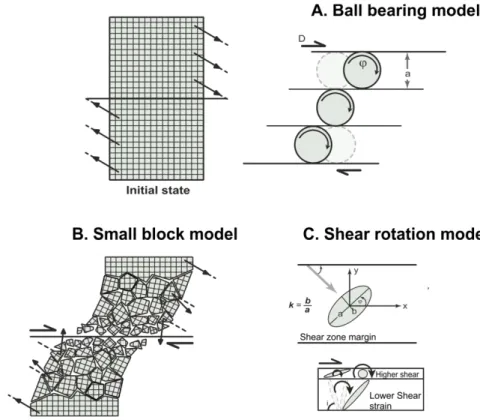
Figure 4. QUASI-CONTINUOUS KINEMATIC MODELS. Modified by Hernandez-Moreno et al., 2014. A) Ball bearing model [Beck, 1976; Piper et al., 1997]; B) Small block model [McKenzie and Jackson, 1983; Nelson and Jones, 1987; Sonder et al., 1994]; C) Shear rotation model

[Lamb, 1987; Randall et al., 2011].

Here the thin viscous sheet represents the ductile middle and lower crusts under the uppermost brittle seismogenic crust, which unlike in the continuous models, is broken into small rigid blocks with sizes smaller than the shear zone width (Figure 4B-5). Block rotations occur in response to the angular velocity of the ductile deformation, taking place at great depth in the lower crust [Beck, 1976; McKenzie and Jackson, 1983; Lamb, 1987; Nelson and Jones, 1987; Salyards et al., 1992; Sonder et al., 1994; Piper et al., 1997; Randall et al., 2011].

The rotation magnitude will depend on fault length, lithosphere rheology, displacement amount, block aspect ratio (short/long axis) and their orientation with respect to the system-bounding fault [Lamb, 1987; Piper et al., 1997; Randall et al., 2011]. The rotation is CW (CCW) in regions of dextral (sinistral) shear, and increases gradually getting closer to the

19

fault, reaching values greater than 90º [Nelson and Jones, 1987; Sonder et al., 1994; Piper et al., 1997].

One of the most simple quasi-continuous models is the ball bearing fashion [Beck, 1976; Piper et al., 1997], where crustal blocks can rotate freely like balls in a bearing into narrow zones bounded by strike-slip faults parallel to the main shear zone (Figure 4A-6). As the rotation is a continue process, brittle destruction at the corners of the blocks tends to produce sub-rounded equidimensional blocks [Hernandez- Moreno, 2015].

The relationship between fault displacement D and rotation φ (expressed as a proportion of 360º) of a fault block of width a approximated by a freely moving circular block is:

𝐷𝐷 = 𝜑𝜑𝜑𝜑𝜑𝜑 (𝟏𝟏)

But rotating blocks are not usually equidimensional, as might be required to accommodate very large rotations prevented by the friction between them [Nur et al., 1986].

Figure 5. Small-block (quasi-continuous model) from Lamb [1987].

Figure 6. Ball bearing fashion model from Beck [1976] and Piper et al. [1997].

20

Since from structural observations, may not be possible to know the block size or size distribution, Sonder et al. [1994] present two block geometry models to estimate the maximum characteristic block size associated with a strike-slip fault (Figure 7).

Figure 7. Models proposed by Sonder et al. [1994] to estimate block size. Arrows indicate

paleomagnetic declinations at hypothetical localities. a) Circular block model, R is the radius

of shaded rigid circular block, r the position of a locality relative to the centre of the block, and L the inter locality distance, 𝑝𝑝̅ (the average probability that a site a distance L from the locality at r is indistinguishable from that at r) is related to the fraction of the circle of radius L inside the rigid block (shaded circle). b) Domain block model. In this case R is the width of the domain, |𝑦𝑦| the distance from the domain axis of a locality, and L the distance of other localities from the first.

The first model (equal blocks rotating independently), considers a rigid circular block of radius R sampled at a distance r from its center (Figure 7a) [Sonder et al., 1994].

The second model concerns to highly elongated blocks rotating together as domains [McKenzie and Jackson, 1983, 1986; Ron et al., 1984; Taymaz et al., 1991a,b] (Figure 7b). Conversely, Lamb [1987] and Randall et al. [2011] in their shear rotation model showed ellipsoidal blocks whose rotation rate and amount are function of both their aspect ratio (k = short axis b/long axis a) and orientation with respect to the system bounding fault through time (Figure 4C). Thus, this model predicts a marked decrease in rotation rate for elongate blocks (k <1, constant) when they rotate into a direction more nearly parallel to the Shear Zone margins [Randall et al., 2011]. Conversely, if the aspect ratio k increases by breakup during rotation (k ~ 1), the resulting equidimensional block will continue to rotate at a constant rate [Lamb, 1987].

21

For a width shear zone W, and fault displacement D, the total amount of rotation at any particular time, given the initial orientation ϕi of the long block axis a, is determined by the

ratio D/W and the aspect ratio k [Lamb, 1987].

The block rotation for k > 5 can be approximated within 10% accuracy to that of a passive marker line, equation 2, while for k ~ 1 is defined by the equation 3 [Lamb, 1987]:

𝜃𝜃 = 90° − 𝜙𝜙𝑖𝑖+ atan (𝐷𝐷/𝑊𝑊 − tan (90° − 𝜙𝜙𝑖𝑖)) (𝟐𝟐) 𝜃𝜃 = 0.5 𝐷𝐷/𝑊𝑊 (𝟑𝟑)

If k does not equal to 1, also there is a simplified expression for R, the instantaneous rotation rate (dϕ/dt), by Lamb [1987]:

𝑅𝑅 =𝑊𝑊_{2 ��}1 − 𝑘𝑘_{1 + 𝑘𝑘}2₂� (cos 2𝜙𝜙 + 𝑡𝑡𝜑𝜑𝑡𝑡𝜃𝜃 sin 2𝜙𝜙) − 1� (𝟒𝟒)

Positive values of R indicate CCW rotations.

When k = 1, R is constant and equals –W/2 (CW to dextral shear). For k < 1, the rotation rate varies with orientation. For sufficiently small values of k, R changes sign for certain orientations and hence the block will rotate in the opposite direction. The overall effect of all this deformation is a “straightening-out” of the major faults, where shear could be taken up by slip on the faults without any rotation of the intervening faults blocks or slow rotation.

The end-member of the quasi-continuous models would be in the case of elongated blocks trending approximately parallel to the relative plate motion across the strike-slip zone. Pure strike-slip is applied to blocks displacing parallel to the deformation zone, implying a lack of rotations [Geissman et al., 1984; Platzman and Platt, 1994; Bourne et al., 1998] (Figure 8).

22

If the frictional forces on faults walls are negligible in comparison with basal traction, the block will be in equilibrium when the net drag force on their base is zero [Bourne et al., 1998]. This coincides with one of the stationary states of Lamb [1987].

Figure 8. Transcurrent deformation by displacement on parallel faults, with no rotation. Modified from Sonder et al. [1994].

24

Chapter

II

25

2. FUNDAMENTALS OF PALEOMAGNETISM

Paleomagnetism [Tarling, 1983; Tauxe, 1998; 2009; Butler, 1992] is a branch of Geophysics that studies the geomagnetic field behaviour of the geological past. It has widespread applications for a variety of disciplines: the study of atmosphere and biosphere interactions, the study of the early history of the Earth [e.g., Tarduno et al., 2006], the physics of the Earth's interior [e.g., Christensen and Wicht, 2007], tectonics [e.g., Torsvik et al., 2008, 2012; Hernandez Moreno et al., 2014; 2016], geologic applications from magnetostratigraphy, biostratigraphy [e.g., Opdyke and Channell, 1996], and archaeomagnetic dating [e.g., Lanos, 2004; Pavòn-Carrasco et al., 2011].

This subject has been vastly addressed in the last forty years by both research papers and books [e.g, Irving, 1964; McElhinny, 1973; Beck 1976, 1980, 1984; McElhinny, 1976; Jelinek, 1977, 1978; Hillhouse, 1977; Simpson and Cox, 1977; Beck and Burr, 1979; Kamerling and Luyendyk, 1979; Coney et al., 1980; Magill and Cox, 1980; Bates et al., 1981; Magill et al., 1981; Globerman et al., 1982; Magill et al., 1982; Demarest, 1983; Merril and McElhinny, 1983; Tarling, 1983; Hillhouse and Grommé, 1984; Coe et al., 1985; Luyendyk et al., 1985; Wells and Coe, 1985; Beck et al., 1986; Grommé et al., 1986; May and Butler, 1986; Hagstrum et al., 1987; Wells and Heller, 1988; Butler et al., 1989; Butler, 1992; Dunlop and Özdemir, 1997; Tauxe, 1998, 2009; McElhinny and McFadden, 2000].

The Earth’s magnetic field is approximately a dipolar field (95% of the field component), resulting from an internal source (the dynamo in Earth’s core mantle and crustal field) and external source (atmospheric field, and crustal induced field; Merrill et al., 1996). The non-dipolar field is that part of internal geomagnetic field, remaining after that dipole contribution has been removed.

26

Assuming the validity of dipolar geocentric field, the geomagnetic field can be represented as a vector framed into a three-dimensional, orthogonal coordinate system usually with origin in a specific point on the earth surface. This vector has an H magnitude and can be broken into

two components, Hv vertical and Hh horizontal (Figure 9). The direction of geomagnetic field

is describe by Inclination I (angle between the horizontal plane and the geomagnetic field

vector, ranging from -90° to 90° and positive when downward) and declination D (angle from geographic north to horizontal component, ranging from 0º to 360º, positive clockwise).

Figure 9. Geomagnetic field H components: Hv vertical component, Hh horizontal

component, I inclination, D declination. Modified after McElhinny [1973].

The vertical component, Hv, of the surface geomagnetic field, H, is defined as positive

downwards and is given by

Hv = H sin I (𝟓𝟓)

where H is the magnitude of H and I is the inclination of H from horizontal, ranging from

–90° to +90° and defined as positive downward. The horizontal component, Hh, is given by

Hh = H cos I (𝟔𝟔)

and geographic north and east components are respectively,

27

where D is declination, the angle from geographic north to horizontal component, ranging from 0° to 360°, positive clockwise [Butler et al, 1998].

Determination of I and D completely describes the direction of the geomagnetic field. If the components are known, the total intensity of the field is given by the equation:

𝑯𝑯 = �𝐻𝐻_𝑁𝑁2 _{+ 𝐻𝐻}

𝐸𝐸2+ 𝐻𝐻𝑉𝑉2 (𝟖𝟖)

A central concept to many principles of paleomagnetism is the Geocentric Axial Dipole

(GAD) model, where the magnetic field produced by a single magnetic dipole at the center of the Earth and aligned with the rotation axis is considered (Figure 10).

The geographic latitude λ is ranging from –90° at the south geographic pole to +90° at the north geographic pole. The inclination of the field can be determined by

tan 𝐼𝐼 = �_𝐻𝐻𝐻𝐻𝑣𝑣

ℎ� = �

2 sin 𝜆𝜆

cos 𝜆𝜆 � = 2 tan 𝜆𝜆 (𝟗𝟗)

and I increases from –90° at the geographic south pole to +90° at the geographic north pole. This relationship between I and latitude will be essential for paleogeographic reconstructions and tectonic applications of paleomagnetism. For a GAD, D = 0° everywhere.

Figure 10. Modified after Butler [1998]. Geocentric axial dipole model. Magnetic dipole M is placed at the center of the Earth and aligned with the rotation axis; the geographic latitude is λ; the mean Earth radius is re; the magnetic field directions at

the Earth’s surface produced by the geocentric axial dipole are schematically shown; inclination, I, is shown for one location; N is the north geographic pole. Redrawn after McElhinny [1973].

28

The magnetic field in a generic point is described by the equation:

B = μ0H + μ0J

where B is magnetic induction (expressed in T), H magnetic field strength (A m–1_{), J}

magnetization (Am–1_{) or magnetic moment per unit of volume.}

In vacuum, J is nil, in matter its properties depend on those of the elementary particles, according to which substances are subdivided into three categories: dia-, para- and ferromagnetic.

The diamagnetic response to application of a magnetic field is acquisition of a small induced

magnetization, Ji, opposite to the applied field, H. The magnetization depends linearly on the

applied field and reduces to zero on removal of the field. Magnetic susceptibility values, χ,

for a diamagnetic material is negative (χ < -10-5 _{SI) and independent of temperature (Figure}

11a). An example of a diamagnetic mineral is quartz, calcite and dolomite.

For Paramagnetic solids, the acquisition of induced magnetization is parallel to the applied field. Magnetic susceptibility values for these materials are positive (10-5_{≤ χ ≤ 10}-3 _{SI) and}

depend on temperature (Figure 11b). For any geologically relevant conditions, Ji is linearly

dependent on H. As with diamagnetic materials, magnetization reduces to zero when the magnetizing field is removed. An example of a paramagnetic mineral are clay minerals, fayalite, Fe2SiO4.

Ferromagnetic substances "sensu latu" are magnetite, titanomagnetites, greigyte. The χ >> 0

and varies in a complex way according to the variation of applied field and temperature (Figure 11c-12). The main characteristic of ferromagnetic substances is a magnetic field of their own, also in absence of an external field H.

In this type of substance, very strong interaction exists at atomic level, called exchange interaction, which favour the orderly arrangement of the dipole magnetic moments. Above a

29

certain temperature, characteristic of each ferromagnetic substance, spontaneous magnetization material fades, and the material becomes paramagnetic. This characteristic

temperature is called the Curie Temperature (TC), instead for anti-ferromagnetic substances

(hematite) is known as Neel Temperature (TN). Based on the size of a single ferromagnetic

granule, it is possible that its internal structure is divided into a series of microscopic volumes each characterized by a preferential direction (and versus) of magnetization J. These regions are called magnetic domains and are developed to minimize the overall magnetic energy of the ferromagnetic granule.

Depending on the size, granules will be:

• Single Domain (SD) (a granule SD of cube-shaped magnetite, has size less than 0.1 μm);

• Pseudo Single Domain (PSD) (a PSD granule of cube-shaped magnetite, has dimensions between 0.1 μm and 1 μm) and

• Multi Domain (MD).

There is another category of ferromagnetic substances called superparamagnetic (SP). A

superparamagnetic granule is a ferromagnetic granule of extremely small size (of the order of 0.01-0.03 μm for magnetite). Because of their dimensions, in order to remove an external magnetic field H, these granules are not able to maintain a remaining magnetization for a long time (paramagnetic substances loose the remaining magnetization instantly). Another feature of these substances is that they have a very high magnetic susceptibility (allowing easy identification) [Butler, 1992].

30

Figure 11. Modified after Butler [1998]. a) Magnetization, J, versus magnetizing field, H, for a

diamagnetic substance. Magnetic susceptibility, c, is a negative constant. (b) J versus H for a

paramagnetic substance. Magnetic susceptibility, c, is a positive constant. (c) J versus H for a

ferromagnetic substance. The path of magnetization exhibits hysteresis (is irreversible), and magnetic susceptibility, c, is not a simple constant.

Figure 12. Modified after Pullaiah et al. [1975]. Normalized saturation magnetization versus temperature for magnetite and hematite. js0 =

saturation magnetization at room temperature; for hematite, js0 ≈ 2

31

Paleomagnetism entails the assumption that the “frozen” magnetization ( primary) during rock formation (consolidation, diagenesis, cooling, etc), by means of several acquisition mechanisms (detrital, thermal, chemical magnetization), is parallel to the contemporaneous geomagnetic field at the time of the formation.

The essential paleomagnetism theory was presented by the Noble prize winner Louis Néel [1949, 1955], who explained how the ancient magnetic field (Banc) might be preserved in

rock’s magnetic memory.

The Néel relaxation theory [1949] defines the characteristic relaxation time (τ) by the equation, which relates τ to frequency factor ( ≈ 108 _s-1_{), volume of single domain grains (v),}

the anisotropy constant (k), the absolute temperature (T) (kT is the thermal energy), the

microscopic coercitive force in single domain grains (hc) and the saturation magnetization of

the ferromagnetic material (js):

𝜏𝜏 =_{𝐶𝐶 𝑒𝑒𝑒𝑒𝑝𝑝 �}1 𝑣𝑣 ℎ_{2𝑘𝑘𝑘𝑘 � (𝟏𝟏𝟏𝟏)}𝑐𝑐 𝑗𝑗𝑠𝑠

The Nèel theory is valid for the single domain grains (SD, i.e. of ~ 0.03 µm with a single and stable domain). Depending on Temperature, the relaxation time can overcome the geological time or be unstable over minutes (as the T closes in the unblocking temperature of magnetic grains the relaxation time decrease exponentially).

The capability of rocks to record a stable remanent magnetization depends on the relaxation time, as stated by the Néel theory [1949, 1955], depending, in turn, from temperature, and volume of magnetic grains [Butler, 1992; Tauxe, 2009].

The original magnetization can be stable along geological times, although rocks may be exposed to other magnetic field, and undergo thermal, chemical processes that can overprint or even remove the primary magnetization, then acquiring secondary remagnetization.

32

Secondary magnetizations can be partial or total, deleting completely the original magnetization. Let's distinguish:

The Natural Remanent Magnetization (NRM) is the remanent magnetization in a rock sample prior to laboratory treatment, and depends on the geomagnetic field and the geological processes occurred during rock formation. NRM is typically composed of different components; a primary component is the component acquired during the rock formation, secondary components are acquired subsequently, altering or even obscuring the primary NRM. The main forms in which the NRM can be recorded are the TRM, DRM and CRM.

The Thermo Remanent Magnetization (TRM) is acquired during cooling from high temperatures to temperatures below Curie Temperatures (temperature below which the magnetic material retains a remanent magnetization (Figure 13); it changes with respect to magnetic minerals).

Figure 13. Modified after Tauxe, 2005; a) Picture of lava flow courtesy of Daniel Staudigel. b) While the lava is still well above the Curie temperature, crystals start to form, but are non-magnetic. c) Below the Curie temperature but above the blocking temperature, certain minerals become magnetic, but their moments continually flip among the easy axes with a statistical preference for the applied magnetic field. As the lava cools down, the moments become fixed, preserving a thermal remanence.

33

The Detrital Remanent Magnetization (DRM) is acquired during the accumulation of magnetic minerals during sedimentation and diagenesis.

The Chemical Remanent Magnetization (CRM) is acquired during the formation (precipitation of ferromagnetic minerals from a solution) of magnetic minerals within a rock, or the alteration of pre-existent magnetic minerals (Figure 14).

Figure 14. Modified after Tauxe [2005]; Grain growth CRM. a) Red beds of the Chinji Formation, Siwaliks, Pakistan. The red soil horizons have a CRM carried by pigmentary hematite. b) Initial state of non-magnetic matrix. c) Formation of superparamagnetic minerals with a statistical alignment with the ambient magnetic field (shown in blue).

Secondary component of remanent magnetization should be detected and rejected (as the

Isothermal and Viscous Remanent Magnetizations - IRM and VRM).

For the interpretation it is critical to isolate the primary and secondary magnetizations and evaluate rocks post-depositional tilting, or folding and other geological processes overprinting the original component of remanent magnetization.

For further details, see reference books by Butler [1998], Lanza and Meloni [2006] and Tauxe [2009].

34

2.1.GEOLOGICAL AND TECTONIC APPLICATIONS

Since decades [e.g. Torsvik et al., 2008, 2012; Hernandez Moreno et al., 2014 and reference therein] the paleomagnetism has played a central role in the solution of tectonic problems from lithospheric plates scale (paleogeographic reconstructions, poles migrations, etc.) to small scale, detecting tectonic motions as rotations with respect to a reference paleomagnetic pole.

The paleomagnetism is the only tool that permits to measure the intensity H, inclination I and declination D of the magnetic field, and therefore deduce all the components of a remanent magnetization of rocks, necessary to detect vertical-axis rotation and latitudinal motion of crustal blocks.

To determine the expected paleomagnetic direction for rocks of any age at any point on Earth surface and then the motions of crustal blocks with respect to the rotation axis, we need to know reference poles. If the measured paleomagnetic declination and inclination are different with respect to those expected, in relation to the geographic position and the age of the analyzed rocks, tectonic rotations can be inferred.

There are two basic methods of analyzing vertical-axis rotations and latitudinal motions from paleomagnetic directions, the direction-space and pole-space approaches. These methods have been developed by Beck [1976, 1980], Demarest [1983], and Beck et al. [1986].

In this work, the direction-space approach is considered, where the observed paleomagnetic direction for a particular site (Io, Do) is simply compared with the expected direction (Ix, Dx)

obtained on rocks of the same age from the stable part of the continent (Figure 15). The inclination flattening or latitudinal motion, F, and the rotation, R, of declination is given by, respectively:

𝐹𝐹 = 𝐼𝐼𝑒𝑒 − 𝐼𝐼𝑜𝑜

35

R is defined as positive when Do is clockwise with respect to Dx.

Both the expected and observed directions have associated confidence cones (α95), so F and R

have 95% confidence limits ΔF and ΔR, respectively. Results of direction-space analyses are usually reported by listings of R ± ΔR and F ± ΔF. A significant positive flattening of inclination, F ± ΔF, indicates motion toward the paleomagnetic pole. To a complete explanation of the confidence limit mathematical development refer to Demarest [1983] and Butler [1992].

Figure 15. Modified after Butler [1992]. a) Equal-areal projection of an observed discordant paleomagnetic direction, inclination Io and declination Do, compared to an expected

direction, inclination Ix and declination Dx. The observed direction is shallower than the

expected direction by the flattening angle F. Observed declination is clockwise from the expected declination by the rotation angle R. b) Comparison of observed and reference paleomagnetic poles. The discordant paleomagnetic pole OP (observed pole) was determined from paleomagnetic analysis of rocks at the collection location labeled S; RP is the reference paleomagnetic pole; the spherical triangle with apices at S, OP, and RP is shown by the heavy lines; pr = great circle distance from S to RP; po = great circle distance from S to OP; poleward transport p = po – pr; vertical-axis rotation R = angle of spherical triangle at S.

This analytical approximation can be used when the 95% confidence cone of the paleomagnetic direction is less than 10º and the mean inclination is not too close to vertical [Clark and Morrison, 1983; Demarest, 1983]. For I >80º the paleomagnetic declination is poorly defined.

36

2.2.MAGNETIC ANISOTROPY

Other important structural information may also come from the magnetic anisotropy studies,

a field also widely investigated in the last forty years [Janák, 1967; Hrouda and Janák, 1976; Jelinek, 1977, 1978; Borradaile, 1981, 1987, 1988; Hrouda, 1982; Borradaile and Tarling, 1984; MacDonald and Ellwood, 1987, Hrouda and Jelinek, 1990; Parés et al., 1999].

Rocks in which intensity of induced or remanent magnetization depends on direction of the

applied magnetic field gain a magnetic anisotropy. One type of magnetic susceptibility (K,

which represents the ratio between the induced magnetization M and the applied magnetic field H) is the Anisotropy of Magnetic Susceptibility (AMS), in which susceptibility is a function of direction of the applied field.

Measurement of the AMS is the technique used to determine the preferred orientation of fine-grained minerals in sediments where no mineral fabric is appreciable to the naked eye (“magnetic fabric”, eg. Owens and Barnford, 1976; Goldstein, 1980; Hrouda, 1982; Borradaile, 1988; Lowrie, 1989; Pearce and Fueten, 1989; Jackson and Tauxe, 1991; Rochette et al., 1992; Sagnotti and Speranza, 1993; Tarling and Hrouda, 1993; Borradaile and Henry, 1997; Bouchez, 1997; Mattei et al., 1997; Cifelli et al., 2005; Pares et a.l, 2015; Caricchi et al., 2016).

The fabric is the result of various forces acting during the formation and eventual geologic history of the rock: mainly gravity, Earth’s magnetic field, hydrodynamic forces and tectonic stress.

The AMS can be geometrically defined as a second-rank tensor, commonly expressed in

terms of a triaxial ellipsoid with its own orientation defined by the directions of the three

37

Figure 16. The magnetic susceptibility ellipsoid. M maximum (or K1- Magnetic Lineation), K

intermediate (or K2), K minimum (or K3 - Magnetic Foliation). Modified after Chadima and

Jelinek [2009].

The AMS ellipsoid principal axes usually correspond to the strain ellipsoid axes, indicating that the magnetic fabric is a strain proxy, and suggesting that magnetic fabric measurements are significant with respect to the strain history of rocks [e.g. Goldstein and Brown, 1988].

Several parameters are used for the quantification of the magnitude of anisotropy and for defining the shape of the AMS ellipsoid [Figure 17; Jelinek, 1981; Hrouda, 1982; Tarling and Hrouda, 1993; Winkler et al., 1997].

Figure 17. Most commonly used AMS parameters (SI units). Modified after Winkler et al., [1997], see references therein.

38

The magnetic lineation (L) and foliation (F) describe the shape of ellipsoid with a geometrical meaning: the lineation corresponds to the direction of K1, the foliation to the plane being defined by the directions of K1 and k2 and hence orthogonal to k3.

When the ellipsoid is prolate (k1>k2=k3) L prevails, and when it is oblate (k1=k2>k3) F

prevails (Figure 18-19).

A more detailed evaluation of the shape of the ellipsoid is given by the Jelinek shape parameter, T, for which -1≤T<0 corresponds to prolate ellipsoids, and 0<T≤1 to oblate ellipsoids [Jelinek, 1981; Figure 19].

Figure 18. Shape of AMS ellipsoids; a) oblate (= planar fabric);

b) prolate (= linear fabric).

Modified after Lanza and Meloni, [2006]

a _b

Figure 19. Flinn diagram [Flinn,1962] . Shape parameter T as a function of lineation (L) and foliation (F). Arrows point towards increasing degree of anisotropy (P). Modified after Tarling and Hrouda [1993].

39

One of the main breakthroughs in the last decade has been the wide recognition of a specific

magnetic mineralogy related to AMS. In particular, there are important mineral sources of susceptibility that are not carriers of NRM (ferromagnetic minerals sensu lato) such as the diamagnetic, paramagnetic, and anti-ferromagnetic minerals, referred to as matrix minerals because they constitute the main volume fraction of common rocks [see detail in Figure 20; Owens and Barnford, 1976; Borradaile, 1987; Rochette, 1987]. The paramagnetic minerals, often play a major role in the magnetic susceptibility of rocks [Rochette, 1987], different from diamagnetic compounds like quartz, calcite or water which do not vary to a great extent, having a mean value of about -14 x 10-6 _SI.

The anti-ferromagnetic matrix behaviour exemplified by goethite and hematite, leads to a linear susceptibility smaller than the paramagnetic susceptibility. According to Neel and Pauthenet [1952], at this point it is worth mentioning a difficulty arising from the present definition of matrix susceptibility: hematite contributes to both the matrix component, with an isotropic anti-ferromagnetic susceptibility, and the ferromagnetic component which is alone responsible for the anisotropy.

Figure 20. Modified after Rochette et al. [1992], see references therein. Selected AMS Data for rock-Forming Minerals.

40

In weakly deformed (non-metamorphic) sedimentary rocks, AMS reflects the pristine fabric produced during incipient deformation at the time of, or shortly after, deposition and diagenesis of the sediment [Sintubin, 1994; Mattei et al., 1995, 1997; Sagnotti et al., 1998, 1999; Parés et al., 1999; Coutand et al., 2001; Cifelli et al., 2004, 2005, 2009; Soto et al, 2009].

AMS analysis of weakly deformed sediments, have frequently been used in orogenic settings to document the syn-sedimentary tectonic regime [Kissel et al., 1986; Mattei et al., 1995, 1997, 1999; Sagnotti and Speranza, 1993; Sagnotti et al., 1998; Parés et al., 1999, 2015; Maffione et al., 2008, 2012, 2015; Macrì et al., 2014; Cifelli et al., 2013, 2015; Caricchi et al., 2016].

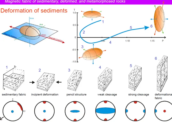
During deposition, sedimentary rocks acquire the so called ‘sedimentary fabric’ characterized by the kmax and kint axes dispersed within a plane (magnetic foliation, the orthogonal plane to

the minimum magnetic susceptibility direction) that is sub-parallel to the stratification plane. This sedimentary fabric can be partially overprinted by a ‘tectonic fabric’ during incipient deformation [e.g., Parés et al., 1999; Alimohammadian et al., 2013]. The result of this process is the development of a magnetic lineation (the direction of maximum susceptibility in a rock)

whereby kmax aligns parallel to the maximum axis of stretching (ε1), hence perpendicular to

the maximum axis of compression (σ1). This mechanism allows a direct correlation between

the AMS and strain ellipsoids [e.g., Parés et al., 1999, 2015].

A series investigations of correlation between the AMS fabric and structural observations,

confirmed that in compressional settings the magnetic lineation is usually sub-horizontal and

parallel to fold axes or local thrusts strikes [e.g. Borradaile and Henry, 1997; Mattei et al., 1997; Sagnotti and Speranza, 1993; Mattei et al., 1997; Sagnotti et al., 1998; Maffione et al., 2008], whereas it coincides with the stretching direction in extensional basins [e.g. Sagnotti et al., 1994; Cifelli et al., 2005; Oliva-Urcia et al., 2009]. In extensional settings, the magnetic

41

lineation coincides with the local dip of the bedding, and is therefore perpendicular to the local normal fault planes [Sagnotti et al., 1994; Mattei et al., 1997, 1999; Cifelli et al., 2004, 2005; Maffione et al., 2012; Porreca and Mattei, 2012]. Few attempts of using AMS analyses in strike-slip tectonic settings have been done in the past [e.g., Cifelli et al., 2013; Ferré et al., 2002].

Increasing deformation progressively modifies the shape of the AMS ellipsoid from a pure sedimentary fabric (oblate ellipsoid: kmax ≈ kint >> kmin), to a sedimentary fabric with a marked

tectonic imprint (triaxial ellipsoid: kmax > kint > kmin), to a tectonic fabric (prolate ellipsoid:

kmax >> kint ≈ kmin), and eventually returning during the highest strain to an oblate ellipsoid

with the magnetic foliation parallel to the cleavage/schistosity [e.g., Parés, 2004, 2015] (Figure 21).

Figure 21. Magnetic fabric evolution during progressive deformation. The ellipsoid is oblate (flattened) when K1»K2 but K2>K3, and prolate (cigar-shaped) when K1> K2, K2»K3. Modified

42

In the last stage of deformation, which corresponds to incipient metamorphism, the pristine tectonic fabric developed during the initial (syn-sedimentary) phases of deformation is completely obliterated. Conversely, the pristine tectonic fabric is not easily overprinted by small strains at low temperature [e.g., Borradaile, 1988; Sagnotti et al., 1994, 1998; Cifelli et al., 2004, 2005; Parés, 2004; Soto et al., 2009]. This implies that, compared to classical structural geological analysis, where the definition of the age of deformation requires additional constraints (i.e., crosscutting relationships or unconformities), the finite strain determined from AMS analyses of weakly deformed rocks is a direct and powerful tool that can be used to study the deformation active at the time of sedimentation.

Sometimes, unusual relationships between structural and magnetic axes, consisting in the “exchange” of the maximum and minimum anisotropy axes (Figure 22, so called inverse

magnetic fabric) can occur because of the presence of certain magnetic minerals, either SD

magnetite, iron-bearing carbonates or various paramagnetic minerals like tourmaline, cordierite, goethite or siderite [Rochette et al., 1992]. Rocks with fine-grained magnetite, are particularly prone to anomalous AMS fabric. Therefore it is strongly recommended to investigate the mineralogical source of AMS and to compare AMS with other types of anisotropy or mineralogical investigation. Accordingly, in the past, authors strongly recommended to investigate the mineralogical source of AMS and to compare AMS with other data of different types of anisotropy or mineralogical investigation.

Figure 22.

Example of Inverse Fabric projection.

43

Chapter

III

44

3. SAMPLING AND LABORATORY METHODS

During this research activity, two field campaigns for sample collection were carried out on April 2016 and 2017, providing a total number of 930 core samples. The samples were collected following a classic paleomagnetic sampling method: several sites have been selected in the same rock unit and several samples in the same site (ca. 10 on average). The samples include volcanic rocks (n. 17 basalt sites) and sedimentary rocks (n. 5 whitish siltstones sites and n. 72 continental red beds).

Sampled sites were aligned along transects cutting the main strike-slip faults considering that several studies demonstrated that shear-related rotations virtually end within 10–20 km from the fault trace [Ron et al., 1984; Sonder et al., 1994; Piper et al., 1997; Randall et al., 2011; Hernandez-Moreno et al., 2014, 2016].

Figure 23. A) Portable petrol-powered drill; B) paleomagnetic sampling; C) Pomeroy orientation device in use as a sun magnetic compass; D) Schematic of the principles of sun compass orientation (by Tauxe, 2005).

A B C

45

The samples were drilled using a portable petrol-powered and water-cooled drill (Figure 23). Cores were oriented in situ before extraction using a magnetic compass, corrected for the local magnetic declination for year 2016/2017 (between 0° and 0.9° W according to NOAA’s National Geophysical Data Center, http://www.ngdc.noaa.gov/geomag/declination.shtml) and, when possible, the sun. Afterward, the cores were cut into standard cylindrical paleomagnetic specimens of 22 mm height.

Paleomagnetic measurements were later carried out in the shielded room of the paleomagnetic laboratory of the Istituto Nazionale di Geofisica e Vulcanologia (Rome), using a 2G Enterprises DC-superconducting quantum interference device cryogenic magnetometer (Figure 24).

Neogene volcanic samples were demagnetized in 10 steps by alternating field (AF) yielded by three orthogonal coils in-line with the magnetometer up-to a maximum AF peak of 100 mT (Figure 24a). Red beds, Jurassic basalts and whitish siltstones samples were thermally demagnetized using a Pyrox shielded oven (Figure 24b) in 12 steps (20°, 200°, 300°, 350°, 400°, 440°, 480°, 520°, 560°, 600°, 640°, 680°C) of temperature up to 680°C. Demagnetization data were plotted on orthogonal vector component diagrams [Zijderveld, 1967].

46

The magnetization components were identified by principal component analysis (PCA) [Kirschvink, 1980] using Remasoft 3.0, a freeware distributed by Agico [Chadima and Hrouda, 2007]. The site mean paleomagnetic directions were computed using Fisher [1953] statistics, and plotted on equal-angle projections. Finally, the rotation and flattening values with respect to Eurasia were evaluated according to Demarest [1983], using the reference paleopoles by Torsvik et al. [2012] for 170-140 Ma sites (Europe), and the most recent East Asia-focused poles by Cogné et al. [2013] for 130 to 10 Ma sites (Figure 25-26).

a b

c

Figure 24. a-c) View of the

magnetically shielded room of the paleomagnetic laboratory (INGV, Rome) and schematic description of samples position into cryogenic

magnetometer ; b) The Pyrox oven

and its controller, to demagnetize up to 700 °C.

47

Figure 25. East Asia paleopoles from Cogné et al. [2013].

48

To define the sense and amount of rotation, have been always considered the smaller angle between the observed and expected declinations, thereby calculating rotation values always ≤|180°|. This is a conservative approach, although we are aware that in the past, some authors considered rotation values exceeding 180° [e.g. Hernandez-Moreno et al., 2014; Nelson and Jones, 1987; Nelson and Piper et al., 1997].

Moreover, for each sampling site, have been selected specimens for additional magnetic analyses carried out with the aim of characterizing the magnetic mineralogy.

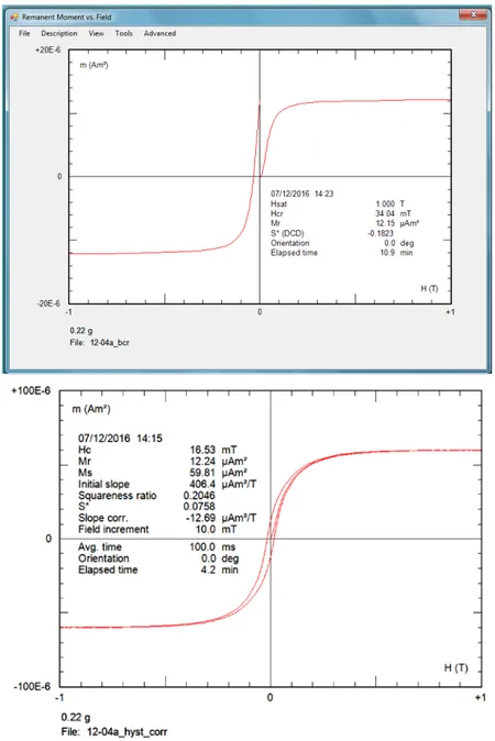
For hysteresis measurements, the samples were crushed into powder and then placed in pharmaceutical gel caps #4 (corresponding to a filled volume of about 0.15 ml), in order to vibrate by means of a carbon fiber probe in the Princeton Measurement Corporation Micromag 3900 Vibrating Sample Magnetometer (VSM) (Figure 27). The software MicroMagVSM was used for hystresis data analysis (Figure 28).

49

Figure 28. Graphic interface of MicroMagVSM program used for data visualization of hysteresis measurements

The coercive force (Bc), the saturation or maximum remanent magnetization (Mrs) and the saturation/maximum magnetization (Ms) were measured using the VSM under cycling in a maximum field of 1.0 T, and determined after subtracting the high field paramagnetic linear trend when saturated samples. The coercivity of remanence (Bcr) values have been extrapolated from the backfield remagnetization curves up to -1 T, following a forward magnetization in +1 T field. Bcr represents the negative field needed to remove the remanent magnetization after applying the maximum positive field. The saturation remanence to

50

saturation magnetization (Mrs/Ms) vs. the ratio of remanent coercive force to coercive force (Bcr/Bc) has been plotted in a Day plot [Day et al., 1977; Dunlop, 2002].

First order reversal curves (FORCs) have been measured using the Micromag operating software, and processed, smoothed and drawn with the FORCINEL Igor Pro routine [Harrison and Feinberg, 2008]. FORCs are a series of partial hysteresis loops made after the sample magnetization is saturated [Pike et al., 1999; Roberts et al., 2000]. Selected FORCs have been measured in steps of 2 mT with an averaging time of 100 ms; the maximum applied field was 1.0 T. The optimum smoothing factor was calculated by the FORCINEL software.

For one specimen from each basalt and red bed sites, have been also measured the variation of the low-field magnetic susceptibility (K) during a heating and cooling cycle performed in air, from room temperature up to 700°C, using an AGICO KLY-3 Kappabridge coupled with a CS-3 furnace (Figure 29). The Curie/Néel points have been estimated as the temperature, or range of temperatures, at which the paramagnetic behavior starts to dominate, following the approach outlined by Petrovsky and Kapicka [2006]. Cureval8 software was used for data analysis (Figure 29).

Figure 29.

Graphic interface of Cureval8 program used for data visualization of thermal curves.

51

Analysis of low-field anisotropy of magnetic susceptibility (AMS) was done using a MFK1 Kappabridge (AGICO) (Figure 30-31). During measurement, the specimen slowly rotates subsequently along three perpendicular axes (total of 64 measurements are made during one spin). The AMS parameters were evaluated using Jelinek statistics [Jelinek, 1977, 1978; see details in chapter II]. Anisoft42 software was used for data analysis [Chadima and Jelinek, 2009] (Figure 32).

Figure 30. AGICO MFK1-FA susceptibility meter, connected to the furnace for measuring the variation of susceptibility vs. temperature.

52

Figure 31. Three specimen positions for the automatic AMS measurements using the rotator.

Figure 32. Graphic interface of the program used for data visualization AMS analysis [Chadima and Jelinek, 2009].

53

Finally, have been also used a tool to apply a pulse magnetic field up to 2.7 T, in order to

impart an isothermal remanent magnetization. This method, called the "Three Axis Method"

or the "Lowrie Method" [Lowrie, 1990], applies to a sample three decreasing fields along

three orthogonal directions (2700 mT, 600 mT and 120 mT respectively from z, y and x axes) using a pulse magnetizer (Figure 33). Then the sample is thermally demagnetized by increasing temperature steps. From the analysis of the demagnetization curves along the three x, y and z components, it’s possible to discriminate the Curie (or Néel) temperatures of distinct ferromagnetic fractions of analyzed sample and characterized by specific coercivity spectrum.

Figure 33.

The 2G pulse magnetizer, the field can reach up to 2.7 T

54

3.1THE FOLD TEST

With the fold test (or bedding-tilt test) can be evaluated relative timing of acquisition of a component of NRM (usually ChRM) and folding. If a ChRM was acquired prior to folding, directions of ChRM from sites on opposing limbs of a fold are dispersed when plotted in geographic coordinates (in situ) but converge when the structural correction is made (“restoring” the beds to horizontal). The ChRM directions are said to “pass the fold test” if clustering increases through application of the structural correction or “fail the fold test” if the ChRM directions become more scattered. The fold test can be applied either to a single fold or to several sites from widely separated localities at which different bedding tilts are observed (Figure 34). The fold test is used to understand when the magnetizations were acquired with respect to the tilting process [Butler, 1992].

Figure 34. Modified after Butler [1992]. Schematic illustration of the fold and conglomerate tests of paleomagnetic stability. Bold arrows are directions of ChRM in limbs of the fold and in cobbles of the conglomerate; random distribution of ChRM directions from cobble to cobble within the conglomerate indicates that ChRM was acquired prior to formation of the conglomerate; improved grouping of ChRM upon restoring the limbs of the fold to horizontal indicates ChRM formation prior to folding. Redrawn from Cox and Doell [1960].