Applied Image Processing Algorithms for Forensic Applications

UNIVERSITA’ DEGLI STUDI DI CATANIA

D

R

M

A

– XXIV ciclo

Tesi di Dottorato

Applied Image Processing Algorithms

for Forensic Applications

Arcangelo Ranieri BRUNA

Tutor Coordinatore

Ch.mo Prof. Sebastiano Battiato Ch.mo Prof. Giovanni Russo

5

7

Acknowledgements

I would like to take this opportunity to thank the whole Image Processing Lab (Catania University), in particular prof. Battiato for his patience and to trust on me.

A special thank is also dedicated to Fausto Galvan and Giovanni Puglisi for the excellent job: thanks to their technical background they allowed the research to proceed faster and in the right direction.

I cannot forget also to thank my family whose patience allowed me to dedicate some of the time I should have spent with them for this PhD.

9

Contents

Preface ... 11

Essential bibliography ... 15

PARTI IMAGE FORGERY DETECTION USING COMPRESSION ARTIFACTS ANALYSIS ... 17

1. Abstract ... 18

2. The driving application... 22

3. The DCT – Discrete Cosine Transform ... 23

4. The JPEG file format ... 26

5. DCT artifacts ... 31

6. Cropping (copy and paste) detection ... 35

Li et al approach ... 36 6.1. Proposed system ... 41 6.2. Experimental results ... 47 6.3. 7. Double quantization detection ... 51

State of the art ... 52

7.1. Scientific background ... 54

7.2. Proposed solution (formula based) ... 57

7.3. Proposed solution (analysis of the histogram of DCT bins) ... 64

7.4. 8. Conclusions and future works ... 86

10

9. Abstract ... 88

10. Introduction... 89

11. State of the art ... 91

12. Validation and classification ... 95

Calibration ... 95 12.1. Training ... 96 12.2. Banknote authentication ... 98 12.3. 13. HW prototype ... 101 14. Experimental results... 104

15. Conclusions and future work ... 106

11

Preface

The research activities described in this thesis have been mainly focused on the analysis and development of techniques able to detect image forgeries. Image Forgery is not only the process to modify an image, but it has a more subjective meaning. A definition could be the following: image forgery is the process of making, adapting, or imitating images with the intent to deceive. It means that an image can become a forgery based upon the context in which it is used. Image manipulation to enhance the visual appearance or to obtain funny images usually cannot be considered forgery, while similar images used to create ambiguous scenario or to discredit someone is a forgery.

The thesis is organized in two main parts: Forensics Image Processing mainly focused on detecting tampering by using compression artifacts analysis and banknote counterfeit detection.

Tampering detection through compression artifacts analysis

Image forgery is not new, but was already performed also in the past with ‘analog’ photography, but it was not simple to obtain realistic images with such techniques, so only few experts were able to create forgeries. Conversely, the digital imaging and the availability of several image processing softwares allow also to inexpert people to obtain good results. There are several kinds of digital forgeries [1]:

 Images created with computer graphics tools (i.e. graphic rendering): these are generated through tools and they are entirely virtuals. Although these tools are very powerful, it is not simple to obtain a ‘realistic’ image, hence only experts are usually able to create deceiving images (i.e. forgeries).

12

 Images obtained by altering the content of a real image: in this case the modifications are obtained by altering some parameters available in any image processing software, e.g., contrast, colors, brightness, etc. The modification can be global or local, just to enhance some particular.

 Images obtained by adding, removing or moving objects. The easiest way is to copy one object from an image and insert it into another image. By manipulating the content, the meaning of the image can drastically change.

There are two methodologies to detect tampered images: active protection methods and passive detection methods [2]. The active protection methods make use of a signature inserted in the image [3]. If the signature is no more detectable, the image has been tampered. These techniques are used basically to assess ownership for artworks and/or related copyrights. Passive detection methods make use of ad-hoc image analysis procedures to detect forgeries. Usually the presence of peculiar artifacts is properly investigated and, in case of anomalies, the image is supposed to be counterfeit.

There is no complete tool helping investigators to detect forgeries, since several techniques counterfeit methods are possible. So the detectives must rely on their experience and apply (usually) semi-automatic methods to retrieve if an image has been tampered.

The first part of the thesis has been devoted to detecting tampering by using compression artifacts analysis. JPEG and MPEG, i.e. the two most used still and video compression standards make use of Discrete Cosine Transform (DCT) engines followed by quantization. It allows obtaining high compression ratio, but, conversely, produces a peculiar artifact. The investigation focused on the characterization of such artifacts and on exploiting such

13 anomalies to detect counterfeits. The most important artifact is the blocking artifact, i.e. a sort of grid superimposed to the original image. This effect is visually visible at higher compression rate, but it can be measured also with low compression ratio. The grid is aligned with the image and has usually the size of 8x8 pixels (in both the directions). Driven by an application aiming to retrieve the original camera model used to shoot the image, two research topics have been targeted: the cropping detection, i.e. the operation that allows obtaining a subpart of the image, and the double quantization detection, i.e. the fact that an image, previously compressed, is opened, modified and hence re-compressed. Moreover techniques aiming to retrieve the first quantization coefficients were also been analyzed.

Image cropping is the technique used to remove unwanted portion of the image. The main effect of the cropping is a misalignment of the regular grid (blocking artifact). Starting from the state of the art algorithms, a new technique has been developed in order to detect if the regular grid is not aligned to the block size (8x8 pixels). This algorithm is very reliable at higher compression ratio while the reliability decreases according to the bit rate, since the blocking artifact is also reduced.

Banknotes counterfeit detection

The detection of counterfeit banknotes is one of the most important tasks in billing machines. Usually it is performed by employing several image analysis techniques (transmittance analysis, reflectance analysis, etc.) on different light spectra (visible, infrared and ultraviolet). Unfortunately these systems are very expensive and are used only for ATM machines where a high degree of reliability is required since those machines are fully

14

unsupervised by humans. In the last years, cheaper systems for validation and classification of banknotes have been commercialized. They are usually based on motors aimed to let the banknote pass through light emitters and sensors in a dark area.

The second part of the thesis is devoted to describe a new system (both hardware and software) for banknote counterfeit detection. The target was to develop a very cheap system without any moving parts (e.g. motors). Users should simply lean the banknote to be analyzed in a flat glass and the system detects forgery, as well as recognizes the banknote value. We used an infrared camera to acquire the banknote enlighten by six infrared Light Emitter Diodes (LED). The infrared light has been used because there are two different inks used in the banknotes with different behavior: one is reflective and one is absorptive. It allows obtaining peculiar images difficult to be counterfeit. In order to obtain a system with high reliability, a lot of problems where handled. First of all the IR light of the LED produces a non-uniform light distribution. It required performing a calibration and a generation of a correction map to be used before image analysis. Moreover the dust in the glass and the high level of noise due to the low light conditions produce very noisy image. Also the banknote position in the glass is a concern, since it produces roto-translation of the acquired image. The last but not the least was the ambient light: since there is no cover in the proscenium, the ambient light (direct light and reflections) cause several problems to the acquired image and, hence, to the image recognition system.

Overall we had also to face with performance constraints: reliability and response time were very tough. It was required to obtain 100% of counterfeit detection, while an amount of false positive were accepted. All the validation and recognition phases should provide results in 2-3 seconds.

15 Unfortunately there were few papers in literature related to banknotes and very few about euro-banknotes. A technique has been deceived using a template matching approach: a training phase allows retrieving a template for each banknote (seven templates for all the banknotes). In order to reduce the effect of the light of the LEDs, a calibration phase allows, for each sample, to detect the light distribution map. During the acquisition process, a pre-processing phase allows compensating for the illuminant and to remove Gaussian noise. The validation phase allows to detect the validity of the banknote and the denomination phase allows obtaining the value of the valid banknote. A hardware prototype has also been developed for real time usage.

Essential bibliography

A. R. Bruna, G. Messina, S. Battiato, “Crop Detection Through Blocking Artefacts Analysis” - International Conference on Image Analysis and Processing (ICIAP) 2011

S. Battiato, A. R. Bruna, G. Farinella, C. Guarnera, “Counterfeit Detection and Value Recognition of Euro Banknotes” accepted in 8th International Joint Conference on Computer Vision, Imaging and Computer Graphics Theory and Applications (VISAPP 2013)

S.Battiato, A.R.Bruna, F. Galvan, G. Puglisi, “A new method to extract the first quantization coefficient in double compressed images” submitted to IEEE International Conference on Multimedia and Expo (ICME 2013), 15-19 July, 2013

S.Battiato, A.R.Bruna, F. Galvan, G. Puglisi, “Double compressed images detection through histogram analysis”, to be submitted to IEEE International Conference on Image Processing (ICIP 2013), 15-18 Sep, 2013

16

S.Battiato, A.R.Bruna, G.Messina, G.Puglisi, “Image Processing for Embedded Devices” - Applied Digital Imaging ebook series (book), eISBN: 978-1-60805-170-0, 2010

S. Battiato, A. R. Bruna, G. Farinella, C. Guarnera, “Counterfeit Detection and Value Recognition of Euro Banknotes” to be submitted to MDPI Sensors — Open Access Journal

17

PART

I

18

1. Abstract

Image Forgery is the process of making, adapting, or imitating images with the intent to deceive. It means that an image can become a forgery based upon the context in which it is used. As example, funny modifications to an image in general cannot be considered a forgery until it is not used, e.g., to extort money. There are several examples in internet. One of the most interesting is http://www.fourandsix.com/photo-tampering-history/.

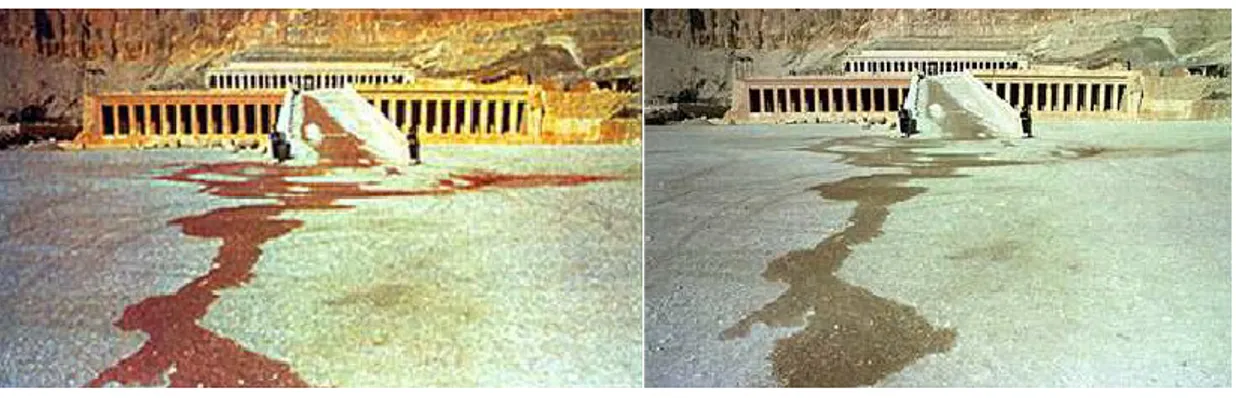
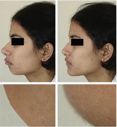
As example, in Figure 1, the intent of the image modification is to hide body imperfections [1]. It cannot be considered a forgery. Conversely, the image in Figure 2 is probably a forgery. Figure 3 is also a forgery since the image was used by a Swiss tabloid to deceive the and to fascinating the readers. Figure 4 instead is not a forgery since in this case the aim is not to deceive someone but to show the customers the benefits of a surgical treatment.

In the last years, the number of forged images has drastically increased due to the spread of image capture devices, especially mobile phones, and the availability of image processing software. Several techniques may be used to tamper an image: copy and paste, filtering, collage of multiple image, etc. are just few examples.

In image forensics it is important to understand (without any doubts) if an image has been modified after the acquisition process.

There are two methodologies to detect tampered images: active protection methods and passive detection methods [2]. The active protection methods make use of a signature inserted in the image [3]. If the signature is no more detectable, the image has been tampered. These techniques are used basically to assess ownership for artworks and/or related copyrights. Passive detection methods make use of ad-hoc image analysis

19 procedures to detect forgeries. Usually the presence of peculiar artifacts is properly investigated and, in case of anomalies, the image is supposed to be counterfeit.

There is no complete tool helping investigators to detect forgeries, since several techniques counterfeit methods are possible. So the detectives must rely on their experience and apply (usually) semi-automatic methods to retrieve if an image has been tampered.

In this thesis are shown methods able to detect tempering by analyzing artifacts due to the compression algorithms. In particular, since the JPEG and MPEG compression schemes are the most used in the world, we focalized on analyzing the effect of the block based DCT transform and quantization of the coefficients. The methodologies are basically stand-alone systems and may be integrated in more complex pipeline, as shown in Figure 5.

20

Figure 1: Funny image that cannot be considered as forgery.

Figure 2: This image manipulation, probably, should be considered as forgery.

Figure 3: After 58 tourists were killed in a terrorist attack at the temple of Hatshepsut in Luxor Egypt in Nov 1997, the Swiss tabloid Blick digitally altered a puddle of water to appear as blood flowing from the temple.

21

Figure 4: In this case the image was modified digitally to show the changes that can be achieved with surgical-orthodontic treatment.

22

2. The driving application

Although the research has been driven to obtain stand-alone systems to detect forgeries in order to be used to detect the single tampering, also a driven application has been chosen by cascading different blocks in order to obtain a complete solution. As example, in Figure 5 there is a block based schema of a system able to retrieve the camera model from an image, after a copy/paste and re-encoding counterfeit process. The proposed solution aimed to handle images without any further compression. In this case, in fact, the further compression may introduce blocking artifact that may deceive the algorithm. In this case, the algorithms described in [4] and [5] can be used for the quantization detection, while the study proposed in [6], [7] can be used for the signature detection block. In particular the image cropping and the re-quantization will be described in this thesis. They could be inserted in a pipeline for complex tampering detection using compression artifacts analysis.

The research was oriented, in particular, to detect forgeries using the file format commonly used by internet and DSC users. Since JPEG is the most used algorithm for still images and MPEG for video sequences [8], we focused on these algorithms and exploit their peculiarities to detect forgeries. Both JPEG and MPEG use Discrete Cosine Transform (DCT) to obtain a high compression ratio preserving visual quality. This is the reason why, in the next chapters, the DCT, the JPEG algorithm and the DCT artifacts are deeply described.

23

3. The DCT – Discrete Cosine Transform

The Discrete Cosine Transform (DCT) [9], [10] and [11] is one of the most used image transformation. It is used to de-correlate the image data in the spatial frequencies. It is similar to the Discrete Fourier Transform (DFT), but has several advantages. It is real (while the DFT is complex), it is simpler to be computed, etc.

There are eight standard DCT variants, of which four are common. The most common variant of discrete cosine transform is the type-II DCT, which is often called simply "the DCT"; its inverse, the type-III DCT, is correspondingly often called simply "the inverse DCT" or "the IDCT". These transformations (DCT and IDCT) are used in some images and video standard compression engines, e.g.: JPEG, MJPEG, MPEG, DV. Moreover there is the modified discrete cosine transform (MDCT), based on the DCT type IV, which is based on a DCT of overlapping data and it is used mostly in audio compression standards, e.g. AAC, Vorbis, WMA, and MPEG-1 audio Layer 3 (known as MP3).

We focused on the DCT and IDCT (i.e. type-II and type-III), since they are used in image and video compression standards.

Formally, the discrete cosine transform is a linear, invertible function (where denotes the set of real numbers), or equivalently an invertible N × N square matrix. The N real numbers are transformed into the N real numbers according to

the formula:

24

Figure 6: Two dimensional DCT spatial frequencies.

Since an image is a 2D matrix, the 2D transform is obtained as a separable product (equivalently, a composition) of DCTs along each dimension, i.e.:

Eq. 2

The kernel is separable, i.e. it is obtained as two application of the 1D DCT twice: first by row and then by column.

It allows reducing the implementation complexity.

The image in Figure 6 shows combination of horizontal and vertical spatial frequencies for an (8x8) two-dimensional DCT. Each step from left to right and top to bottom is an increase in frequency by 1/2 cycle. For example, moving right one from the top-left square yields a cycle increase in the horizontal frequency. Another move to the right yields two

half-25 cycles. A move down yields two half-cycles horizontally and a half-cycle vertically. The source data (8x8) is transformed to a linear combination of these 64 frequency squares.

26

4. The JPEG file format

JPEG is acronym of Joint Photographic Expert Group [12]. It is the most used still image compression standard algorithm for both low quality images (i.e. the images used in internet) and high quality images (i.e. the images acquired by the digital still cameras) [8], and resisted also to ‘attacks’ of other standards, e.g., the JPEG2000 [13].

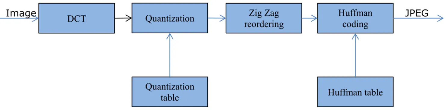
The Figure 7 shows the block based schema of the algorithm.

The image is supposed to be described in YCrCb format (i.e. luminance and chrominance). The chrominance components may also be subsampled, since the visual impact of the lossy information is negligible.

Every component (both luminance and chrominance) is divided into 8x8 pixels blocks. Each block is transformed in the DCT domain according to a modified formula described in the previous Section 3:

Eq. 3

where

 is the horizontal spatial frequency, for the integers .  is the vertical spatial frequency, for the integers .

 is a normalizing scale factor to make the

27

Figure 7: Block based schema of the JPEG standard.

 is the pixel value at coordinates  is the DCT coefficient at coordinates

Compared to the DCT in Section 3, this formula makes the DCT-II matrix orthogonal (i.e. the transpose matrix is the inverse matrix), but breaks the direct correspondence with a real-even DFT.

It is used to de-correlate the 64 coefficients in the spatial frequencies, so each one of the coefficient can be elaborated independently using a visually weighted quantization matrix. The quantization coefficients are the main cause of the loss of information. In Figure 8 is shown the quantization matrix for the luminance and chrominances proposed in the Annex K of the JPEG standard [22]:

DCT

Image _Quantization Zig Zag

reordering Huffman coding Huffman table JPEG Quantization table

28 [ ] [ ]

Figure 8: Standard proposed quantization matrix used for the luminance (Y) and the chrominance (C).

[ ]

Figure 9: Example of quantization table optimized for landscapes.

The quantization step is performed according to the following formula:

(

) Eq. 4

The standard does not impose to use the quantization table shown above, so the quantization values can be chosen depending on the desired compression ratio [14], [15],

29 [16]. Optimization of the coefficients may be performed depending on several aspects: image acquisition sensor, target bit rate, image category (e.g. portrait and landscape), etc [17]. In Figure 9 an example of quantization table optimized for landscapes is shown.

It is important to remark that every image acquisition system uses, in general, its own quantization tables. This information can be used to retrieve the camera model even if it is not directly shown in metadata [6], [7].

The coefficients of the quantized blocks are then reordered according to a zig-zag ordering method shown in Figure 10. It allows obtaining a 1D vector of coefficients ordered according to the spatial frequency, in particular from the lowest frequency (called DC) to the highest frequencies (called AC).

The particular scanning allows obtaining, statistically, nonzero values at the beginning of the vector and a long run of zero coefficients. Finally the chain is encoded using a run-length/variable length encoder through a Huffman table. The Huffman table is not standardized, but can also be optimized, i.e., according to the image content [18]. This process allows modifying the bit rate, but it is a time consuming methodology and the benefit in terms of compression ratio improvement is not enough, so it is not usually used by commercial systems in real time.

30

31

5. DCT artifacts

The DCT, as stated above, is the widely used image transformed domain for image and video compression since it provides better tradeoffs between image quality and compression ratio. Increasing the compression ratio, the quality, of course, decreases. Several artifacts are generated at lower quality, since they are the result of discarding a relevant amount of information represented by DCT coefficients once they have undergone the lossy quantization process. Usually these are side effects. But, since they are well known and widely studied, they can also be used to detect if a compression schema has been applied to an image.

The most known artifacts are [44], [45] and [46]:

 Blocking  Ringing

 Color bleeding

Blocking artifact is the most known artifact. It appears as small square blocks all over the

images. It is due to the fact that JPEG and MPEG compression engines work with 8x8 blocks, one at a time. An example is shown in Figure 11.

32

Figure 11: Example of blocking artifact.

Ringing artifact is a distortion of edge appearance. DCT based compression schemes, in fact,

operate in spectral domain, trying to represent the image as a sum of smooth oscillating waves. Spectral domain is appropriate for capturing relatively smooth color gradients, but not particularly appropriate for capturing edges. So, instead of capturing an edge as it is, the edge is fitted with wave functions. Further quantization step produces loss of detail and, especially in strong edges, produces this artifact. An example is shown in Figure 12.

33

Figure 12: Example of ringing artifact.

Colour bleeding artifact appears as a smearing of the colour between adjacent areas of

strongly contrasting chrominance. This phenomenon can be observed in both still images and videos. The phenomenon is due to the combination of quantization and decimation (mainly 4:2:0 sub-sampling), which introduces spurious information on the reconstructed signal; hence no bleeding is usually observed when the two signal degrading processes are not simultaneously applied. An example of such artifact is visible in the Figure 13.

34

Figure 13: Example of color bleeding artifact.

Usually these artifacts are unwanted effects and a lot of algorithms have been developed to reduce them. In image forensic they can be used to detect if tampering methods have been used.

35

6. Cropping (copy and paste) detection

Copy and paste is the simplest technique used to counterfeit images. It can be used to obtain a completely new image by cropping the interest part or to cover unwanted details.

Several algorithms exist in literature as reported in a recent survey [4]. Among others, a lot of methods in the field consider the possibility to exploit the statistical distribution of DCT coefficients in order to reveal the irregularities due to the presence of a superimposed signal over the original one [4], [5], [20], [21]. The DCT artifacts analysis have a further advantage due to the fact that it is the most used compression technique; JPEG [22] for still images and MPEG compression family [23] for video sequences make use of block based DCT data compression (usually 8x8 pixel size non-overlapping windows).

While there are a lot of algorithms in literature for the estimation of the quantization (and compression) history [4], [5], there are only a few approaches for cropping detection [21]. In this Section a pipeline is suggested aiming to merge both techniques in order to obtain a more reliable system. In fact, blocking artifacts analysis works well when the image is aligned to the block boundary. But, in case the image has been cropped, this assumption is no more valid and the detection may fail. In the Figure 5 the quantization detection block is preceded by a cropping detection in order to align the image to the block boundary. It allows to increase the reliability of the detection and to better understand if only some parts of the image are tampered.

In Li et al. [2] the grid extraction is realized by extrapolating the Block Artefact Grid (BAG) embedded in the image where block artefact appears, i.e. the grid corresponding to the blocks boundaries. The authors introduce a measure of blockiness just considering the ratio between the sum of AC components of the first raw (and column) with respect to the DC

36

coefficient in the DCT domain. One of the main drawbacks of the method is related to the fact that it requires to compute 8x8 pixels DCT again (in a dense way) over the image under detection, just to locate properly the correct alignment. Also the detection of tampered regions corresponding to misaligned grid is demanded to a visual inspection of the resulting filtering operation without a clear and objective measure.

The same authors propose in [21] an interesting approach based on spatial consideration devoted to locate the BAG just combining together a series of derivative and non-linear filters to isolate blockiness avoiding the influence of textures or strong edges present in the input image. Unfortunately, both the techniques were not properly evaluated just considering a proper dataset (high variability with respect to resolution size) and a sufficient number of misalignments cropping with respect to the 8x8 grid. Also an exhaustive comparison just considering the overall range of JPEG compression factors is lacking.

As described in [4], [24] the new emerging fields of Digital Forensics require to provide common benchmarks and datasets that are needed for fair comparisons among the numerous proposed techniques and algorithms published in the field. The same authors suggested a third approach in [25] that overcome some problems of the previous and will be described deeply in the next Section.

Li et al approach

6.1.

One of the most interesting approaches related to the detection of copy and paste detection of pre-quantized images is the Li et al approach [25]. They define “Block Artifact Grid” (BAG) as the grid embedded in an image where block artifact appears.

37

Figure 14: Example of BAG misalignment.

The DCT grid and BAG match together in undoctored images. When an image slice is moved, the BAG within it also moves. In Figure 14 there is an example showing the mismatch of the BAG with the DCT grid when a slice is copied and pasted in another image area.

Li proposed an algorithm to detect the BAG misalignment. It locates the BAG firstly, and then checks whether the BAG mismatches or not with the DCT grid. Once a BAG mismatch is detected, then the image can be considered doctored. It is based on the assumption that the high frequency AC coefficients of every 8x8 DCT block are usually zero after quantization in a pre-compressed image. When no copy and paste operation occurred, high frequencies coefficients of all the blocks are zero, otherwise some values are not zero, since BAG is not aligned. It is basically an anomaly and it is a cue of copy and paste operation. Even when the texture is complex and some high frequency coefficients are not zero, the misaligned BAG may be also detected.

As example a 1D example will be considered. To locate the BAG, an error measure was defined, as shown in the following formula:

38

| | Eq. 5

Where is a predictive value while is the signal and i is the index in the range

[0,length(signal)]. Since high frequency DCT coefficients are usually zero, the prediction can

be obtained by imposing the 7th coefficient to be zero too, as shown in the following formula:

[∑

]

Hence the prediction value can be computed as:

∑ ( )

Eq. 7

Sliding the window along the sequence, the error effect is calculated. An example is shown in Figure 15. It is visible that the minimum of the values appear at the block edges.

The extension to the 2D case is straightforward: assuming the block to be 8x8 (as usual for JPEG standard), suppose the luminance signal and are the corresponding DCT

coefficients:

39

Figure 15: Example of 1D BAG signal and correspondent error function.

Then the local effect is defined by using the last column and row AC coefficients of each block:                         77 76 75 74 67 66 65 64 73 72 71 70 63 62 61 60 50 41 40 07 06 05 04 30 20 10 03 02 01 00 p p p p p s s s p p p p s s s s s s s p s s s s s s s s s s

Since the 2D DCT is composed by:

Eq. 9

There are 15 undetermined coefficients. By imposing:

( ) Eq. 10

40

The formula can also be expressed as a matrix equation:

[ ][ ] [ ] ( ) Eq. 11

Where:

( ) ( ) Eq. 12

And

∑ ∑ ( ) ( ) Eq. 13

Thus the predictive coefficients can be calculated as:

[ ] [ ] [ ] Eq. 14

Finally, the local effect can be defined as the root-mean square prediction error:

√

∑ ( ) ∑ ( )

Eq. 15

Sliding the window in the whole image, the map of error E can be obtained as the BAG. The lower values (darkest point if showed as image) correspond to the BAG. In the Figure 16 an example of the process is shown.

41

Figure 16: Lena image and the corresponding Block Artifact Grid (BAG) image.

Proposed system

6.2.

The DCT codec-engines (e.g., JPEG, MPEG, etc.) typically apply a quantization step in the transform domain just considering non-overlapping blocks of the input data. Such quantization is usually achieved by a quantization table useful to differentiate the levels of quantization adapting its behavior to each DCT basis. The JPEG standard allows using different quantization factors for each of the bi-dimensional DCT coefficients. Usually standard quantization tables are used and a single multiplicative factor is applied to modify the compression ratio [26],[27], obtaining different quality levels. As the tables are included into the image file, they are also customizable as proved by some commercial codec solutions that exploit proprietary tables. Images compressed by DCT codec-engines are affected by annoying blocking artifacts that usually appear like a regular grid superimposed to the signal. In the following, we discuss a simple example based on the Lena image [43]. The picture has been compressed using the cjpeg [26] software with a properly managed

42

Figure 17: Blocking artefact example in a JPEG compressed image (quality factor = 40).

compression ratio, obtained modifying the quantization tables through the variation of the quality parameter in the range {10, 90} (see Figure 17).

It is an annoying artefact visible especially in flat regions. It is also regular, since it depends on the quantization of the DCT coefficients of every 8x8 blocks.

Unfortunately, this kind of artefact is not simple to be characterized (i.e., detectable) in the Fourier domain, since image content and the effect of the quantization step of the encoding pipeline mask the regular pattern, as shown in Figure 18.

43

Figure 18: Results of the visualization of the Fourier spectrum applied to the compressed Lena image shown in Figure 17.

We established to work directly in the spatial domain and, in particular, in the luminance component. The blocking artefact is basically a discrepancy in all the borders between adjacents blocks. It is regularly spaced (8x8 for JPEG and MPEG) and it also affects the image in only two perpendicular directions (horizontal and vertical if the image has not been rotated).

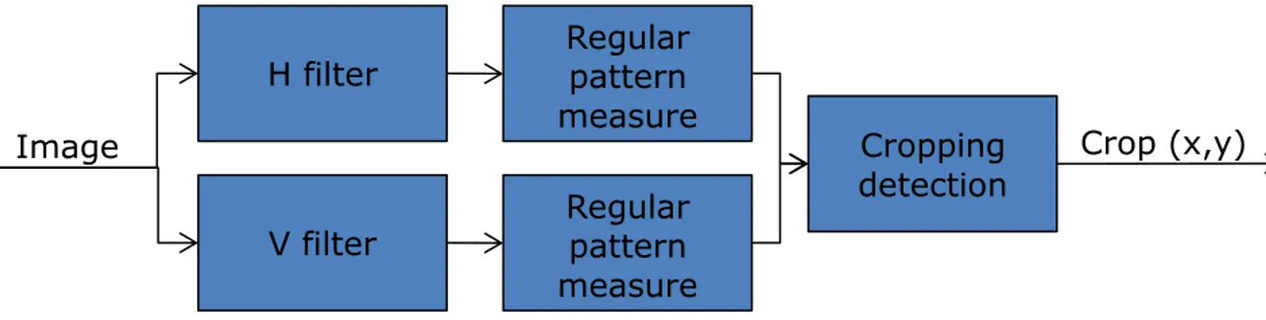
The straightforward way to detect such artefact exploits a derivative filter along the horizontal and vertical direction. The proposed strategy could be easily generalized to consider all possible malicious rotation of the cropped image, just iterating the process at different rotation angles. In Figure 19 the overall schema of the proposed algorithm is depicted.

44

Figure 19: Block based schema of the cropping detection algorithm.

Figure 20: Effect of the Sobel filter (3x3 kernel size) applied to the Lena image.

The blocks “H filter” and “V filter” are derivative filters. Basically they are High Pass Filters (HPF) usually used to isolate image contours. An example is the Sobel filter, with the following basic kernel:

; 1 2 1 0 0 0 1 2 1              H ; 1 0 1 2 0 2 1 0 1               V Eq. 16

These filters are able to detect textures, as shown in Figure 20. H filter Image Regular pattern measure Cropping detection Crop (x,y)

V filter Regular pattern measure

45 It is very useful to retrieve textures of the image, but the blocking artefact effect is also masked. In order to detect only regular pattern and discard real edges, a very long taps directional filter has been used It was obtained by properly expanding the following 3x3 filters along the horizontal or vertical direction:

; 0 0 0 1 1 1 1 1 1               H ; 0 1 1 0 1 1 0 1 1               V Eq. 17

Bigger is the number of taps, better are the results, although computational time also increase. In Figure 21 is shown the result of a long directional filters with different kernel size.

We define the Regular Pattern Measure (RPM) that computes a measure of the blockiness effect as defined in the following. Let I a MxN pixel size image and IH , IV the corresponding filtered images obtained by applying a directional HPF as above. For sake of simplicity let suppose to have serialized the image, by simple scan line ordering of the corresponding rows and columns just obtaining the vector IH’, IV’ . The RPM values for both directions is obtained as:







46







Figure 21: 30 taps directional HPF applied to the Lena image. Borders are not considered (thus the vertical size in the left image and the horizontal size in the right images are less than the original size).

Experiments have shown that both the RPMH and RPMV measures allow discriminating, in a

very robust way (e.g., with respect to the main content of the image), the periodicity of the underlying cropping positions. Such values can be extracted by considering a simple order statistic criterion (e.g., the maximum). Figure 22 and Figure 23 show the plot of the two RPM measures, in case of no cropping (e.g., blocking artefact starts with the pixel [1,1]) and in case of malicious cropping at position [6, 5].

47

Figure 22: RPM measure without cropping. The blocking artefact starts with the pixel [1,1].

Figure 23: RPM measure with cropping. The blocking artefact starts with the pixel [6,5].

Experimental results

6.3.

To assess the effectiveness of any forgery detection technique, a suitable dataset of examples should be used for evaluation. According to [24] the input dataset contains a number of uncompressed images organized with respect to different resolutions, sizes and camera models. Also the standard dataset from Kodak images and from UCID v.2 have been used. The overall dataset can be downloaded from [28]. It is composed by 114 images with different resolution. Experiments were done varying in an exhaustive way the cropping position and the compression rate.

0 2 4 6 8 6 7 8 9 10 11 12 13x 10

4 _{regular vertical pattern measure}

0 2 4 6 8 0.8 0.9 1 1.1 1.2 1.3 1.4x 10

5_{regular horizontal pattern measure}

0 2 4 6 8 6 7 8 9 10 11 12 13x 10

4 _{regular vertical pattern measure}

0 2 4 6 8 7.5 8 8.5 9 9.5 10 10.5 11 11.5x 10

48

Moreover the cjpeg [26], (i.e., the reference code for the JPEG encoder), has been used to compress the images and the flag -quality was used to modify the quality from 10 (high compression ratio) to 90 (low compression ratio) with the step of 10. In particular each image has been cropped in order to test every possible cropping position in the 8x8 block, just to consider the possibility to test the method also in presence of real regular patterns in the image that could influence the results. In Table 1 are reported the overall results, described in terms of correct percentage of the cropping position detection, with respect to the involved compression ratio.

Table 1: Results of the proposed method.

Quality factor Accuracy (%)

10 99 20 91 30 80 40 69 50 58 60 46 70 39 80 28 90 16

Exhaustive tests have been done for every image, every cropping position and quality factor. Thus the accuracy has been obtained considering 2891 cases.

49

Figure 24: RPM measure obtained at varying the quality factor.

Experimental results show that performances increase according to the compression rate. It is reasonable, since the blocking artifact increases at higher compression ratio.

In Figure 24 the RPM (only vertical) measure is shown at varying the quality factor (real crop position = 7). Reducing the quantization (i.e., increasing the quality factor), the peak is less evident and, in this example, with the quality=80 the estimation fails, since the effect of a real edge becomes predominant.

50

Figure 25: Li’s method [1, 7] applied to Lenna image at varying the quality factor.

The proposed solution was compared to the method described in [2] [21]. Unfortunately in these papers the cropping detection is not automatic, but it is supposed a visual inspection at the end of the process. In Figure 25 are shown the results of this method at varying the quality factor from 10 to 90 for the Lena image for a cropping position (3,5). It is evident that the cropping position is detectable up to q=40. Above this value it is no more visible. Similar results have been obtained for all the involved dataset.

Lenna - q=10; crop=(3,5); Lenna - q=20; crop=(3,5); Lenna - q=30; crop=(3,5);

Lenna - q=40; crop=(3,5); Lenna - q=50; crop=(3,5); Lenna - q=60; crop=(3,5);

51

7. Double quantization detection

In the forensic domain it is important to recover image history, i.e. the camera that acquired the image and any further modification (cropping, filtering, merging with other images, etc.). One of the steps is to detect whether or not an image has been doubly compressed, since every (malicious) modification needs the user to decompress the image, to perform the modification and to save it again.

This is not a clear indication of forgery, but it tells us that the image, probably, is not the one originally saved at the time of the shooting. In literature, algorithms can be found able to detect if double quantization occurs. They are based on the analysis of anomalies in the DCT coefficient distribution. Unfortunately, there are no methods able to retrieve in a robust way the coefficients of the first compression in a double compressed JPEG image. It could be useful, e.g., to detect the camera model used for capturing the image. In the following Sections we report methods able to obtain these coefficients exactly when the second compression is lighter than the first one. In these approaches we do not only use anomalies of the compression engines, but we rely also on the peculiar statistical distribution of the DCT coefficients. It is well known, in fact, that the AC coefficients are distributed according to a Laplacian distribution [20]:

( ) Eq. 20

Where:

√

Eq. 21

52

Figure 26: An example of Laplacian distribution.

In Figure 26 there is an example of Laplacian distribution.

State of the art

7.1.

The pipeline which leads to ascertain whether an image has undergone to some kind of forgery leads through the following steps: determine whether the image is “original” and, in the case where the previous step has given negative results, try to understand the past history of the image. Discovery that the input image has been manipulated or not is a prelude to any other type of investigation. Regarding the first stage, the EXIF metadata could be examined, but they are not so robust to tampering, so that they can give us indicative but not certain results. To discover image manipulations, many approaches have been proposed in literature (JPEG blocking artifacts analysis [29], hash functions [30], etc.). A lot of works have proved that analyzing the statistical distribution of the values assumed by the DCT coefficient is widely more reliable [20]. In this regard, as reported in [31], [4] and [32], by checking the histogram of these values we are able not only to determinate

53 whether the image was or not doubly saved, but also if the quantization coefficient, in this case, was greater than or less the one of the first compression. In [5], the authors suggest a method that helps to determine whether an image has been subjected to double compression with the same compression factor. The part of this theory not yet fully developed, at least in our knowledge, concerns the determination of the values of the coefficients of the first quantization. In our approach we focused on the determination of these coefficients. In particular we demonstrate that, when the second quantization factor is lower than the first one, the performed estimation is without doubts, i.e., it also allows detecting the forgery.

From here on, q1 and q2 will indicate respectively the coefficient of first and second

quantization for a generic frequency in the DCT domain. In [33] the author, to estimate q1,

proposes to carry out a third quantization and then calculates the error between the coefficients before and after this step. By varying the coefficient of the third quantization he is able to detect two minima, one (absolute) in correspondence of q2, and one (local) in

correspondence of q1. We will discuss in detail the results of this method and its limitations

in the remainder of this Section, which is structured as follows: in Section 7.2, after a brief review of the JPEG compression algorithm, we present the mathematical details of our new method, we will explain why we are able to find q1 when q1> q2, and also because this

method cannot bring to the same good results in the case where . In Section 7.3 the effectiveness of the proposed solution has been tested considering both synthetic and real data (uncompressed images) reproducing a double quantization in order to simulate the lossy part of the JPEG algorithm.

54

Scientific background

7.2.

The JPEG compression engine [34] works just considering a partition of the input image into 8x8 non-overlapping blocks (for both luminance and chrominance channels). A DCT transform is then applied to each block; next a proper dead-zone quantization is employed just using for each coefficient a corresponding integer value belonging to an 8x8 quantization matrix [20]. The quantized coefficients obtained just rounding the results of the ratio between the original DCT coefficients and the corresponding quantization values are then transformed into a data stream by mean of a classic entropy coding (i.e., run length/variable length). Coding parameters and other metadata are usually inserted into the header of the JPEG file to allow a proper decoding. If an image has been compressed twice (i.e., after having introduced some malicious manipulation) although, of course, the current quantization values are available, the original (initial) quantization factors are lost. It is worth noting that in forensics application, this information could be fundamental to assess the integrity of the input image or to reconstruct some information about the embedded manipulation [35].

For sake of simplicity, considering a single DCT coefficient c and the related quantization factors q1 (first quantization) and q2 (second quantization), the value of each coefficient is

given by:

( ( ) ) Eq. 22

To infer the value of q1, previous works suggest to quantize again such value with a

quantization coefficient (q3) varying in a certain range [33] and to evaluate an error function

55 ( )

( ( ( ( ) ) ) ( ( ) ) )

Eq. 23

For examples, taking an image from [36], the outcome, considering the DC term when q1= 23 and q2= 17, is shown in Figure 27 (a). In this particular case (both coefficients are prime

numbers) we obtain interesting results: both q1 and q2 can be easily found, since they

correspond to the two evident local minima. Hence, in this specific example, the first quantization coefficient q1 can be retrieved (q2, as mentioned before, is already available).

Unfortunately, in real cases, the original quantization coefficient cannot be easily inferred as reported in the following:

 Considering the quantization values used before (q1= 23, q2= 17) and the same input

image, but varying q3 in the range [1:70], the outcome is more complex to analyze

than before. Several local minima arise and a strong one can be found in 65 (see Figure 27 (b)).

 Considering the same input image and q3 in the range [1:30], but with different

quantization coefficients q1 = 21 and q2 = 12 (they are both not prime numbers), the

outcome reported in Figure 27 (c) is obtained. Without additional information about the input image, a wrong estimation could be performed (for example q1 = 28).

56

(a)

(b)

(c)

Figure 27: Examples of error function values vs q3 for the triple quantization: (a) q1 = 23, q2 = 17 and q3 is in

the range [1:30]; (b) q1 = 23, q2 = 17 and q3 is in the range [1:70]; (c) q1 = 21, q2 = 12 and q3 is in the range

57 When q3 = q2, the error function Eq. 23 is equal to zero. This motivates the absolute minima

found in the previous examples.

Finally, the Eq. 23 allows estimating q2, but this information is not useful since q2 is already

known from the bitstream. Obtaining reliable q1 estimation from Eq. 23 is a difficult task

because too many cases must be considered. In the following an alternative strategy able to sensibly increase the reliability of the estimation is then proposed.

Proposed solution (formula based)

7.3.

As explained above, Eq. 23 allows obtaining q2 (already present in the header data) but is

not able to provide a reliable estimation of q1. To solve this problem we have designed a

new error function:

( ) ( ( ( ( ( ) ) ) )

( ( ) ) ) Eq. 24

To properly understand the behavior of Eq. 24, especially when q3= q1, we have to better

analyze the effect of a single quantization and de-quantization step. If we examine the behavior of the following function:

( ) Eq. 25

We can note that if q is odd, all integer numbers in [ ( ) ( )] will be mapped in nq (with n a generic integer number). If q is even it maps in nq all the integer

58

Figure 28: The effect of quantization and de-quantization for coefficient q1.

numbers in [ ]. From now on we call this range ‘space attributable to nq’. We can see an example of this in Figure 28 when q is even.

As a consequence of this behavior, we can say that Eq. 23 “groups” all integer numbers of its domain in multiples of q.

It is very important to observe that the maximum distance between a generic coefficient c and the corresponding ̂, obtained by the quantization and de-quantization function, is if c

is even, ( ) if c is odd. Based on the above observation, we analyze three rounds applied in sequence, when q2< q1 and q3= q1:

( ( ( ) ) ) Eq. 26

 ( ) for the above observations leads to the situation shown in

Figure 28;

 ( ) maps multiples of q1 in multiples of q2. It is worth noting that,

being q2< q1, a generic nq1 will be mapped in a multiple of q2 (for example mq2)

whose distance from nq1 will be less than or equal to (or ( ) if q2 is odd),

59

Figure 29: Scheme describing the effect of three quantization and de-quantization with coefficients q1,

q2 and q3 = q1 again.

 at this point, ( ) maps c2 in nq1 again, since, as pointed out in the

preceding paragraph, c2 is in the space attributable to nq1.

With the three steps above, we demonstrated that, as shown graphically in Figure 29:

( ( ( ) ) ) ( )

Eq. 27

Therefore the error function in Eq. 27 is zero when q3 = q1 regardless the c value.

7.3.1.

Experimental results

In order to prove the effectiveness of the proposed approach several tests and comparisons have been performed. A first test has been conducted considering artificial data. Specifically, a random vector of 5000 elements has been built by using a uniform

60

distribution in the range [-1023:1023]. The range corresponds to an input image within the range [0:255] in the spatial domain. In fact, the output of the DCT transform, as it is defined, is three bits wider of the input bit depth and it is centered in zero. These simulated DCT coefficients are then used as input of the error function (Eq. 27) by considering several pairs of quantization coefficients with q1 < q2. As can be easily seen from Figure 30 (a, b and c),

Eq. 27 has a global minimum (equal to zero) when q3 = q1. Moreover, q1 value can be found

in the range ] [. It is worth noting that, sometimes, more than one local minimum can be found in the range ] [. For example, this behavior can arise when q1 is a multiple of q2 (see Figure 30 (d)). However, even in this case, the correct q1

value can be easily found. In fact, the additional minima are always between q1 and q2 and

their positions depend on the common divisors between q2 and q3. Hence, in this case, q1 is

61

(a) (b)

(c) (d)

Figure 30: Examples of error function values vs q3, computed by using the proposed solution Eq. 24: (a) q1 =

23, q2 = 17 an q3 is in the range [1:30]; (b) q1 = 23, q2 = 17 and q3 is in the range [1:70]; (c) q1 = 20, q2 = 12 an

q3 is in the range [1:70]; (d) q1 = 40, q2 = 20 an q3 is in the range [1:70].

Further tests and comparisons have been performed by simulating a double compression process on real uncompressed images. Specifically, we randomly selected a photo from the Kodak image dataset [36] composed by uncompressed images, we divided it into 8x8 blocks of pixels and, for each block, we computed the DCT. Later, considering all the computed blocks of DCT coefficients, we collect in a vector the elements with the same relative

62

position in the block. The obtained vector has been then double quantizated and dequantizated, with two values q1 and q2 (where q1 > q2), randomly generated in a range of

values [1:30]. Finally, starting from the double quantized vector, we evaluated both the error function Eq. 23 related to [33] and the proposed one Eq. 24. As can be easily seen from Figure 31 the proposed error function outperforms the one proposed in [33] providing, in all the considered cases, a clear global minimum (equal to zero) in correspondence of q3 = q1. On the contrary, obtaining q1 values from Eq. 23, analyzing their

local minima, is a difficult task (see, for example, Figure 31 (g)). Moreover, in some cases, the correct solution does not correspond to a minimum of Eq. 23 as in Figure 31 (c).

As already stated before, the proposed error function has a local minimum (equal to zero) when q3 = q1 and the correct solution has to be looked for in the range ] [ (q2 is

already available). However, in some conditions, other minima could appear. For example, we have already described the behavior reported in Figure 31 (b and f) (q1 is a multiple of q2), that can be easily solved considering the maximum q3 element with zero value. Other

conditions can also produce additional zeros. Specifically, the distribution of the DCT coefficients, depending on the image content, can influence the final results (see Figure 31 (e, i and l)). Although in these cases we obtain more than a candidate (at most 3 in our experiments), the correct q1 value corresponds to the maximum one.

63

Figure 31: Test on real image dataset. The proposed function Eq. 24 is able to better estimate the q1

64

Proposed solution (analysis of the histogram of

7.4.

DCT bins)

In this paragraph a methodology to detect double quantization is explained. It is also able to reconstruct some coefficients of the original quantization matrix. It is based on the analysis of the histogram of bins of the dequantized DCT coefficients.

In particular it is based on the assumption that the quantization step projects the original space of the original DCT data in a subspace composed by a lower number of bins. A further quantization (i.e. double quantization) reduces more and more the cardinality of the new subspace.

In the Figure 32 an example of the histogram before and after a first and a second quantization is shown.

The same concepts explained in 7.3 are used for this method: the original DCT values span in the integer values; the values after the first quantization span in a subset (multiple of the quantization step); the values after the second quantization span in the subset depending on both the first and second quantization values. After Huffman decoding and de-quantization steps, the histogram can be used to detect the first de-quantization coefficient.

In order to better explain the process, the graphs shown in the Figure 32 will be better described: The first graph shows the histogram of the DCT data after the DCT and rounding operation. All the integer bins are filled, i.e. all the integer values spanning theoretically in the range [ ]. It is also important to observe that the histogram has a Laplacian distribution. It is a well-known behavior of the distribution of the AC coefficients [20], as described in Section 7. The second graph shows the histogram of the same image after the

65 first quantization and de-quantization. All the available bins are multiple of the quantization step (10 in this case). Each non zero bin (t) contains all the original values spanning in the range [t-q1/2, t+q1/2]. The third graph shows the histogram after the second quantization

and de-quantization. In this case the bins are not all the multiples of the second quantizer (in this case 6), but some values are missed. As example, the bin 24 is zero because it should contains the bins, before the second quantization, in the range [21, 27], but these values are not multiple of the first quantization table (i.e. 10), so the bin is empty.

The proposed solution makes use of the available non zero bins and the analysis of the anomalies in the histogram of the decompressed image to detect if double quantization occurred. Some values of the original quantization matrix can also be reconstructed. Since the bins are symmetrical respect to the zero value, the absolute value allows increasing their numbers and, hopefully, filling empty bins (see Figure 33).

66

Figure 32: Quantization and double quantization effects on DCT data. Bins are accumulated in few coefficients (multiple of the quantization value). Double quantization produces some anomalies in the dequantized bins. -150 -100 -50 0 50 100 150 200 0 50 100 150 200 Rounded DCT coefficients DCT data H is to gr am -150 -100 -50 0 50 100 150 200 400 600 800 First quantization/de-quantization (q1=10) dequantized coeffs H is to gr am -200 -150 -100 -50 0 50 100 150 200 400 600 800 Second quantization/de-quantization (q2=6) dequantized coeffs H is to gr am

67 The idea is based on the following rationales:

1. Each non zero bin (k) is multiple of the second quantization step (see Figure 32); 2. The needed information can be extracted only through non zero bins analysis.

3. The symmetry of the histogram and the algorithm allows to consider the absolute value of each bin (see Figure 33).

4. The zero bin does not provide any information for the quantization value estimation. 5. Every non zero bin (k) collects all the coefficients of the first quantization step laying

in the interval [k-q2/2, k+q2/2].

Based on these assumptions, it is possible to build an iterative method to retrieve, for every position in the 8x8 grid of the block, the quantization coefficient of the first compression. Since some bins will not be available, especially for the highest frequencies, some coefficients will not be recovered uniquely. This method allows also providing a probability level of each of the reconstructed coefficient. In the following the methodology is explained. Examples will refer to the histogram in Figure 33 obtained by quantizing the DCT coefficients (0,2) with q1=10 and q2=6.

68

Figure 33: The histogram considered as example for the following paragraphs. Only the absolute value is taken into account.

It considers the absolute values of the bins. Moreover all the nonzero bins are taken into account. They are sorted and the list of each entry is taken into account only once. In this example the list of nonzero bins is:

{ }

Every bin ( ) allows detect a list of candidates for the original quantization value. Based on the rationale (5) described previously, we have:

69 Where ̅is the estimated quantization value, and is the second quantization value

(known). It means that the estimated values are not necessarily unique. As example, for

n1=12 and q2=6 we will have:

̅ { [ ] [ ] [ ] [ ] Eq. 29

For n2=18 and q2=6 we will have:

̅ { [ ] [ ] [ ] [ ] Eq. 30

For n3=30 and q2=6 we will have:

̅ { [ ] [ ] [ ] [ ] Eq. 31

This process may be iterated for all the ( ) available bins. For any set of { } with , it is possible to estimate if there is one or more quantizer values that is a possible quantizer value as the intersection of the corresponding sets of values. As example, for the possible first quantizer coefficient is in the following range:

70

̅ {[ ] [ ] [ ]} [ ]

for the possible first quantizer coefficient is in the following range:

̅ {[ ] [ ] [ ]}

That means that this is not a possible set. By varying all the possible there are several allowed set. The possible values for the first quantization coefficient are the union of all the non-empty set.

It is possible to formalize this process.

A single set of values for a given set of can be formalized as:

̅ ( ̅(

)

̅(

)

̅(

))

Eq. 32

Then, for each set of values obtained with the Eq. 32, the first quantization coefficient belongs to the union of all the non-empty set.

Generalizing:

̅ ⋃(⋂ ̅( )) Eq. 33

This formula was implemented with an iterative method. The result, for each bin, is a collection of one or more candidates.

It is to be noted that the retrieval may be done for each of the 8x8 block position, hence 64 times for luminance and 128 for chrominance. In order to detect if a double quantization occurred, it is enough to detect only one coefficient where ̅ is not null.

The methodology may be also used to reconstruct the entire first quantization table, as described in the following Section.

71

7.4.1.

Quantization matrix reconstruction

The method described above allows retrieving a value or a set of values for each of the 8x8 quantization coefficient. It allows reconstructing the first quantization value as the collection of ̅ values with only one value. It allows detecting without any doubt the original quantizer. The other coefficients, i.e. the set containing more than one value, are due to lack of information (i.e. few nonzero bins). In this case we may choose one of these values according to a heuristic methodology. In case of uncertainty, the probability of the estimation is ( ̅).

A possible heuristic is also described in the next Section.

7.4.2.

Experimental results

The method described above has been implemented in Matlab. It was tested by using the image database in [36]. In this Section is shown the results obtained with one of the image of the database, in particular kodim13.png.

72

Figure 34: Kodim13.png, the image used for the tests shown in this Section.

The image was quantized first with the following quantization table:

[ ]

The second quantization is the following:

[ ]