Università degli Studi di Catania
Scuola Superiore di Catania
International PhD
in
ENERGY
XXIII cycle
Adsorption Machine & Desiccant Wheel based
SOLAR COOLING
in a Second Law perspective
Santo Bivona
Coordinator
of
PhD
Tutor
Prof. Alfio Consoli
Prof. Luigi Marletta
1
FOREWARD 3
1. SOLAR COOLING SYSTEM: AN OVERVIEW 5
1.1. Introduction 5
1.2. Conventional cooling technology in a Second Law perspective 5
1.3. Solar technologies for cooling 8
1.3.1. Closed-cycle systems 8
1.3.2. Open-cycle systems 9
2. INTRODUCTION TO EXERGY ANALYSIS 9
2.1. The First Law of Thermodynamics 10
2.2. The Second Law of Thermodynamics 11
2.2.1. The Gouy-Stodola equation 12
2.2.2. The dead state 13
2.3. The concept of exergy 13
2.3.1. Exergy and Anergy 14
2.3.2. Exergy efficiency 16
2.3.3. Exergy of humid air 17
3. SOLAR COOLING SYSTEM DESIGN AND ANALYSIS 18
3.1. System overview and main components description 18
3.2. Dynamic model and simulations 21
3.3. Simulation results 29
3.4. Energy analysis and plant sizing 41
3.4.1. Thermal loads 41
3.4.2. Fan coil 42
3.4.3. Adsorption machine 43
3.4.4. Dry cooler 43
3.4.5. Thermal solar collectors and gas boiler 44
3.4.6. Results of energy analysis 45
3.5. Exergy analysis 46 3.5.1. Solar collectors 47 3.5.2. Boiler 47 3.5.3. Heat storage 48 3.5.4. Dry cooler 49 3.5.5. Fan coil 49 3.5.6. Adsorption machine 51
3.5.7. Results of exergy analysis 51
3.5.8. Global exergy efficiency indexes 55
3.6. Comparison with a conventional HVAC system 56
2
4. USE OF A DESICCANT WHEEL IN HVAC SYSTEM 66
4.1. Desiccant systems 66
4.2. System layout 67
4.3. Desiccant wheel characterization 69
4.4. System analysis 83
4.5. Final results 92
5. CONCLUSIONS 100
3
FOREWARD
The energy demand for summer conditioning is rising year by year due to new massive installation of small/medium size electrical chiller for commercial and residential buildings. Electrical chillers are characterized by low price, easy and quick installation and can provide both cooling and heating if used as heat pumps. On the other hand they need relevant amount of electrical power to operate. This leads to high consumption of fossil fuels for power production, which results in high emission of greenhouses gasses and risk of electricity grid overload.
To find new solutions for air conditioning, research activities are focused on exploiting solar energy for cooling purposes. Fig. (I) shows the cooling and heating loads and the course of the solar radiation during the 12 months of the year. The maximum of the solar radiation occurs in the peak of the cooling load. Therefore, it appears obvious that, using a thermally driven machine and suitable solar collectors, it is possible to take advantage of the solar system for cooling purposes.
Fig. (I) Cooling (in blue) and heating (in red) loads.
Solar cooling plants are supposed to be able to:
- Reduce summer electrical consumption and risk of grid overload and black-out.
- Reduce greenhouse gas emission and air pollution due to fossil fuel utilization.
4
This thesis investigates on exploiting solar energy to provide air conditioning for a small office room. Two different systems based on sorption materials will be analyzed from the First and Second Law point of view, in order to be compared in terms of main features, performance and limits of use.
Plant layout design parameters will be assessed after a number of simulations in dynamic condition, involving solar collectors type and area, heat storage and different system control strategies. Results can be compared in terms of energy performance to find the best compromise between performance and predicted cost. Thus, by means of the First and Second Law analysis, the main figures of merit will be assessed.
A rather new HVAC plant layout, based on a desiccant rotary wheel (solar DEC), will be also analyzed. A mathematical model will be developed and implemented in a computer code in the MathCAD environment, to predict the thermodynamic conditions of air streams at the outlet of a desiccant wheel.
This will allow the simulation of the solar DEC and its analysis in a First and Second Law perspective.
The sensitivity theory will be also applied in order to investigate the systems response to deviations of some state variables from their nominal values. In this context a number of sensitivity coefficients will be determined in relation to the most relevant design parameters. That provides useful information for control strategies in dynamic regime and hints for systems design and optimization.
5
1. SOLAR COOLING SYSTEM: AN OVERVIEW
1.1. Introduction
The most recent surveys ascertain that the demand for building cooling has been increasing in the past few years and will continue to do so dramatically in the near future. The AUDITAC study showed that in 1990 about 10,000 GWh of primary energy were consumed in Europe by
small Room Air Conditioners (RAC) (<12 kW) with 540 Mm2 (million square meters) of
cooled floor area and that in 2020 this value is expected to increase by a factor of four to
about 44,000 GWh, with a cooled area of 2,400 Mm2. Although high, this value does not
include centralized systems, generally installed in large commercial buildings.
The reasons for such a forecast in the cooling demand are several, but mostly due to the more and more popular tendency of modern architecture to use glass façade surface areas, higher demand for comfort, quantitative increase of office and service buildings, increasing number of electric appliances and, in one word, expected economic growth.
All that implies energy, economic and environmental consequences. The technologies currently available are those based on electrically driven compression chillers and thermally driven sorption chillers. Actually, with electric chillers being dominant, the concern is about electricity consumption and, more importantly, black-out risks which may occur in large urban areas, when several thousands of small and large size air-conditioning units are likely to be activated almost simultaneously during the hottest hours of the day in the summer season. Solar cooling systems may help alleviate this problem, considered that the peak cooling demand in summer is synchronous with solar radiation availability.
But there are also different kind and perhaps more substantial reasons which should encourage the shift to new technologies, such as those based on thermodynamic considerations.
1.2. Conventional cooling technology in a Second Law perspective
Air conditioning for the summer season mostly relies on cooling and cooling is mostly based on either electrically-driven or thermally-driven chillers. The energy indicator for both is the
6
well known Coefficient of Performance (COP) which, for the two technologies, is defined respectively as: el th el g Q Q COP COP P Q = =
being Q the cooling power (useful effect), Pel the electricity required to drive the chiller and
Qg the thermal power offered to the generator of the thermal (or sorption) chiller. Actual
values for the COP lay in the following range: COPel = 2 ÷ 4; COPth = 0.6 ÷ 1.2.
On the basis of these numbers one should not conclude that electric chillers are better than thermal chillers, because such a comparison is not properly stated. Indeed the two definitions of COP refer to energy of different quality: heat (Qg) for the sorption machine and electricity (Pel) for the compression machine. A more rational basis for comparison is the Primary Energy Ratio, defined as the ratio of the delivered useful cold (Q) to the Primary Energy (PE) consumption to drive the machine:
Q PER
PE
=
The PE in the currently accepted definition is energy that has not been subjected to any conversion or transformation process, therefore one may consider fossil fuels as sources of PE. As a result, the PER may be assessed by combining the previous equations, such as:
el el el th th g
PER =COP PER =COP
being el = Pel / EP the efficiency of the electric system (nationwide efficiency) and
g = Qg / EP the efficiency of the boiler driving the sorption chiller. Rough numbers may be
as follows: hel = 0.40 (recommended value for Europe); hg=0.90, thus:
PERel=(2÷4) 0.4=0.8÷1.6 and PERth = (0.7 ÷ 1.2) 0.9 = 0.63 ÷ 1.08.
Looking at these results one may conclude that current technologies for cooling are quite acceptable, and in certain cases (for PER > 1), apparently able to provide the user with a cooling energy even greater than the exploited PE. Of course there is no violation of the
7
physics laws, since COPs do not include, by definition, the energy taken from the environment.
A quite different picture appears when one looks at the problem from a second law perspective. In this case we have to judge the technologies on the basis of the exergy efficiency, defined as the ratio of the exergy required by the end-use to that exploited to drive the system. Now the purpose is to extract from the building the heat Q in order to maintain the interior spaces at temperature T
(e.g., T = 26 °C = 299 K) against an outdoor (environment) temperature To(e.g., To= 33 °C =
306 K).
For an electric chiller the exploited exergy is Pel (electric energy is pure exergy). For a sorption chiller, the thermodynamic potential which drives the machine may be assessed as
Qg (1– To/Tg). The maximum temperature Tg of the energy source, for a chiller powered by a
conventional gas boiler, may be assumed equal to the flame temperature (e.g., Tg= 1,500 K).
In formulas: (1 ) 306 ( 1) 3( 1) 7 % 299 306 (1 ) ( 1) ( 1) 299 0.7 2% 306 (1 ) (1 ) (1 ) 1500 o a o el el el a o o a a th th o o g g g T Q T T COP P T T T Q T T COP T T Q T T = = = = = = = =
The results reveal that, under the light of the 2nd Law, the current technologies for cooling are not as good as described, via COP and REP, by the first law. The poor exergy efficiencies tell us something about the improper use we make of the energy sources in this field. The sad thing is that these technologies are also the most widespread in the world and involve both the civil and the industrial sectors.
8
1.3. Solar technologies for cooling
The system under consideration are generally divided into two main categories: close and open cycles.
1.3.1. Closed-cycle systems
These types of systems are based mainly on the absorption cycle. In its simplest, single-effect configuration, an absorption system employs a refrigerant expanding from a condenser to an evaporator through a throttle. A second working fluid is the absorbent. When heat is supplied to the desorber, it absorbs refrigerant vapor from the evaporator at low pressure, and desorbs into the condenser at high pressure. The absorption system is hence a heat-driven heat pump; the heat may come from a variety of sources, including solar. The system operates between two pressure levels, and interacts with three heat reservoirs at various temperature levels: at low temperature in the evaporator; at the intermediate temperature (ambient conditions) in the absorber and condenser. Currently the most common absorbent-refrigerant pairs are LiBr-water and LiBr-water-ammonia.
Single-effect absorption systems have a limited COP: about 0.7 for LiBr-water and 0.6 for ammonia-water, with consequences in terms of solar collector area. Better performance can be achieved by using a higher temperature heat source and a double stage design. In this case high temperature collectors, such as evacuated tube or concentrating collectors must be used. The higher cost of the cooling machine and the solar collector should hence be considered. Double stage absorption chiller may have COP as high as 1.0-1.2, while triple-effect, although still under development, may achieve COP of about 1.7. These systems may be adapted to and employed in a solar-powered installation with high temperature solar collectors. The single stage system requires temperature in the range 80-100°C; for a higher supply temperature, it is worth switching to a double stage system, up to about 160°C, and then to a triple-effect. As to the cooling power, only very few systems are commercially available in the in the range of small capacities (< 100 kW), whereas much more manufacturers offer products for large capacities up to several thousands kilowatts.
9
Adsorption chillers working with solid sorption materials are also available. For a continuous operation it is necessary to work with two or more adsorbers, in such a way that when the first is the desorption the other in the adsorption phase. Adsorption systems allow for somewhat lower driving temperatures but have a somewhat lower COP compared to absorption systems under the same conditions. Silica gel or zeolite adsorption machines with cooling capacities of about 75 kW to several hundreds kilowatt are now available but with very limited application on the field. The noiseless operation and the use of environmentally friendly working fluids ( mostly water ) are further advantages of this technology.
1.3.2. Open-cycle systems
Open-cycle systems are based on the use of desiccant materials which may be liquid or solids. The cycle is “open” in the sense that the refrigerant is discarded from the system after providing the cooling effect and new refrigerant is supplied in its place in an open-ended loop. In this type of systems air cooling and dehumidification is not obtained by means of chilled water, but by specific treatments to the supply (or process) air streams. The solid or liquid sorbent is regenerated with ambient or exhaust air heated to the required temperature by the solar heat source.
For systems using solid sorption material such as silica gel, it is usual to employ a rotary bed carrying the sorbent material, referred to as a 'desiccant wheel', to allow continuous operation. Systems employing liquid sorption materials are less widespread but also available on the market. An interesting feature of desiccant materials is that they have the possibility of energy storage by means of concentrated hygroscopic solutions, as well as bacteriostatic qualities.
2. INTRODUCTION TO EXERGY ANALYSIS
In this chapter the main differences between First and Second Law analysis will be assessed. The concept of exergy, which leads to a different perspective in developing a system performances evaluation, will be shown. At the same time the equation needed to proceed with the air conditioned system analysis will be pointed out.
10
2.1. The First Law of Thermodynamics
When dealing with energy balances, the First Law of Thermodynamics is usually taken into account. It states that energy is a conservative property; this means that during any real steady-state process the overall energy flow leaving a system equals the overall energy flow entering the system.
Actually, the different forms of energy (thermal, mechanical, internal, potential, kinetic) may individually undergo quantitative changes, but the overall amount of energy is conserved. The energy balance equation, which quantifies the energy conservation law for a stationary process observed through a control volume, may be stated as follows:
k entrata k uscita k k w z g h m w z g h m P Q = + + + + 2 2 2 2 & & & (2.1) Where:
• Q& = thermal energy flow crossing the system boundaries [W] • P = mechanical power crossing the system boundaries [W]
• m&= mass flow rate entering / leaving the system [kg/s]
• z = height of the system above a reference level [m] • w = mass flow velocity [m/s]
• h = specific enthalpy measured at the system inlet and outlet [kJ/kg]
The index of performance derived from such an approach compares the amount of energy required by the final user (either electric, or mechanical, or thermal) to the total amount of energy exploited by the system, expressed as:
system the to provided Energy user the to release Energy =
One must realize that such a definition compares different forms of energy. As an example, in
the case of a power plant for the production of electric energy, the energy efficiency ( el) is
11 th el el Q P & =
where Pel is the electric power, and Qth the thermal energy to drive the system.
But, as a matter of fact, different forms of energy have different potentials to produce useful work. So the definition of efficiency stated above is a comparison between quantities which are metrically homogeneous but not conceptually equivalent.
2.2. The Second Law of Thermodynamics
The Second Law of Thermodynamics may help overcome this drawback, on the basis of a rather different approach to system analysis.
The starting point is that real processes are not reversible and give rise to entropy production: friction, hysteresis, molecular or thermal diffusion are the most common examples of irreversibilities occurring in a real process. The mathematical form of the Second Law most suitable for our purposes is the Clausius equation:
(
)
(
)
= j j Outlet k Inlet k T Q s m sm& & & (2.2)
where:
• m&= mass flow rate [kg/s]
• s = specific entropy content [kJ/(kgK)];
• Q& = heat transfer occurring through the system boundaries [W]
• T = temperature of the environment being involved in the heat transfer [K]
• = overall entropy production due to irreversibility [W/K]
As stated by the Second Law, S 0, being = 0 only for ideal (reversible) processes. This relationship is precious, as it allows the assessment of entropy production , which is always the unknown of the problem. It is intuitive that when dealing with complex systems, it is possible to decompose them into several, more simple subsystems; by evaluating for each one of them, it is possible to detect the ones most responsible for thermodynamic drawbacks and thus provide corrective measures.
12
2.2.1. The Gouy-Stodola equation
The first law contains a term for work, but no term for irreversibility, whereas the second law contains a term for irreversibility but not for work. Combining the first and the second law statements allows to state a more general equation than the previous ones. Before doing this it is appropriate to adopt the following expressions:
+ = + = j j j j j T Q T Q T Q Q Q Q 0 0 0 (2.3)
Being Qothe heat transfer to the environment and Toits temperature.
By combining equations (2.1) and (2.2) and taking into account eq. (1.3), one obtains the Gouy-Stodola equation: 0 2 0 2 0 0 2 2 1 m h T s w gz m h T s w gz T T T Q P outlet k k inlet k k n n n + + + + +
= & & & (2.4)
For an ideal reversible process (T = 0), the Gouy-Stodola equation yields:
+ + + + + = outlet k k inlet k k n n n id gz w s T h m gz w s T h m T T Q P 2 2 1 0 & 0 2 & 0 2 & (2.5)
For all real processes T > 0, thus Pid > P, in other terms 0
0 >
= T
P
Pid (2.6)
This means that irreversibilities erode the thermodynamic potential of the energy flows; in other words, at the end of the process or at the system outlet, the energy flows have a lower potential to produce work, and this reduction is measured by the entropy production To. This term is also referred to as “Irreversibility”:
0
T
13
2.2.2. The dead state
The work potential of a system at a given state may be assessed by letting the system proceed towards and actually reach a stable equilibrium with the environment. In fact, when the system and the environment are in equilibrium, no further change of state can occur spontaneously and hence no further work can be produced.
When such a situation occurs, the system is said to be in the dead state. Specifically the dead
state is characterized by conventional values for pressure po and temperature To. Additional
requirements for the dead state are that the velocity of the fluid stream is zero (wo= 0) and the
gravitational potential energy is zero (zo = 0). These restrictions of pressure, temperature,
velocity and elevation characterize the restricted dead state, associated with the thermomechanical equilibrium with the environment. It is restricted in the sense that the chemical equilibrium with the environment is not considered, that is the control mass is not allowed to pass into or react chemically with the environment.
The problem of the chemical equilibrium with the environment will be dealt with later on.
2.3. The concept of exergy
Exergy is defined as the work potential of a system relative to its dead state. Following this definition, for each term appearing in eq. (2.5), it is possible to derive an expression for exergy.
Exergy of (mechanical. or electrical) work:
P
EP = (2.8)
Exergy of heat Q available at temperature T:
=
T T Q
EQ 1 0 (2.9)
14
(
)
(
)
+ +(
)
= 2 02 0 0 0 0 2 g z z w w s s T h h m Em & (2.10)So for a control volume, eq. (2.4) may be rewritten in terms of exergy, as follows:
( )
EP outlet( )
Ep inlet =( )
EQ inlet( )
EQ outlet +( )
Em inlet( )
Em outlet To (2.11)And rearranging the terms:
(
EP +EQ +Em)
inlet =(
EP +EQ +Em)
outlet + T0 (2.12) Therefore: = inlet outlet k j E E T0 (2.13)The irreversibility can then be quantified as the difference in exergy measured at the inlet and outlet of the control volume.
2.3.1. Exergy and Anergy
Considering a given amount of thermal energy Q available at the temperature T allows to state that: = T T Q EQ 1 0 (2.14)
EQ can be thought of as the maximum work which can be extracted from a Carnot cycle,
receiving the heat Q and working between the temperatures T and To . By rewriting the
equation in the form:
T T Q Q
15
it is easy to recognize Q as the amount of energy available at the beginning, and T T
Q 0 as the
amount of energy rejected to the environment as thermal waste; at these conditions, energy is no longer recoverable for technical purposes. Some Authors refer to this quantity as “not available energy” or Anergy.
Similar considerations can be made in relation to the mass flow, where:
The exergy content is:
(
)
(
)
(
0)
2 0 2 0 0 0 2 g z z w w s s T h h + +
The energy content is:
(
)
(
0)
2 0 2 0 2 g z z w w h h + +
The anergy content is: T0
(
s s0)
All forms of energy at the dead state are anergy. The natural environment is an infinite reservoir of anergy. Distinction should be made between anergy and irreversibility. The former has always existed, the latter results while a process is occurring. Irreversibility is anergy which arises whenever a physical event takes place.
Anergy may enter the control volume and then grow by addition of the irreversibilities. Eventually the anergy flow will join the irreversibility flow, so that at the system outlet the anergy results higher than it was at the inlet.
To summarize the previous results, the following relationship can be stated between energy, exergy and anergy :
Anergy Exergy
Energy = +
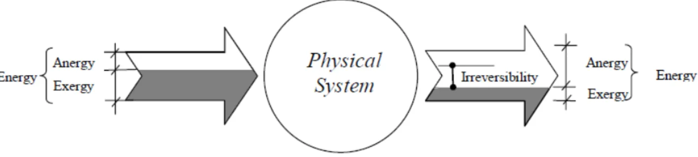
A pictorial view of the concepts outlined so far is provided in Fig. 2-1. Its message is clear: going through the physical system, the exergy flow is lowered by the entropy production, the anergy flow increases by the same quantity, while the energy flow remains constant.
16
Fig. 2-1Exergy and anergy flows across a physical system.
In conclusion, by using the exergy and anergy concepts, the first and second law of thermodynamics may be reformulated as follows:
• in any process the sum of exergy and anergy remains constant;
• in any real process the exergy decreases and the anergy increases by the same quantity as the entropy production;
• the anergy cannot be converted into exergy.
2.3.2. Exergy efficiency
According to this approach, the thermodynamic figure of merit for a process in a second law perspective is the exergy efficiency, defined as:
input Exergy output Exergy = In formulas: inlet inlet outlet inlet outlet E T E T E E E 0 0 1 = = = (2.16)
The exergy efficiency is thus a ratio between quantities that now are both metrically and conceptually homogeneous. The numerical values of never exceed unity. The maximum exergy efficiency ( = 1) is only achievable by ideal systems ( = 0).
17
2.3.3. Exergy of humid air
The availability of a mixture of substances at a given temperature and pressure (T, p) is the maximum work obtainable by bringing the stream to the thermo-mechanical equilibrium with the environment.
Some common energy engineering processes have a mass interaction with the environment, in the sense that the mass may be released to the environment and/or have chemical reactions with it.
In the realm of the HVAC, a relevant case of chemical interaction with the environment is the diffusion process. This process occurs, for example, when the exhaust air is released to the outside from conditioned rooms or when the condensed water is dripping out from a cooling coil.
On the other hand, humid air is a binary mixture of dry air and water vapour; of course everyone of these components has its own thermal, mechanical and chemical interaction with the environment. In order to analyze these processes in a second law perspective, it is necessary to take into account the chemical potential of the constituents, since it is different from that of the environment.
After reaching the mechanical, thermal and chemical equilibrium with the environment, the system is said to be in the ultimate dead state.
The concept of chemical equilibrium involves the calculation of the chemical potential of substances and an extensive theoretical treatment, which is not the case to go through here: the interested reader is referred to the specialized literature.
Actually, the problem of psychrometric processes in terms of “available energy” was first stated and solved by Wepfer, Gaggioli and Obert in a fundamental article published in 1979 [2]. They derived the basic equation for the humid-air streams availability by re-writing the Gouy-Stodola equation, in a proper way for HVAC applications, stating that the global availability is obtained by summing up the thermomechanical and the chemical availability. By doing this, one obtains the following relationship for the evaluation of the exergy of a humid air stream, as a function of pressure p, temperature T, and absolute humidity x:
(
)
(
)
(
)
(
)
0 0 0 0 0 0 0 0 1 , , ln 1 ln 1 ln ln 1 a pa pv a a x T p x e T x p c x c T T T x R T R T x x T p x x + = + + + + + + + (2.17)18 where:
• x= x/0,622;
• Cpa is the dry air specific heat; • Cpv is the water vapour specific heat; • Rais the gas constant for the dry air;
The reference condition (ultimate dead state), denoted with the subscript “0” is usually
assumed to be that of outdoors; therefore: xo= xE; To= TE; po= pE; eE = eo= 0. The exergy of a water flow rate, when kinetic and potential terms can be disregarded, reduces to:
(
)
0 0 0 0 pwln v oln pw w RT T T c T T T c e = (2.18)where cpw is the specific heat for liquid water, Rvthe water vapour constant and othe relative
humidity for the reference state ( o =V E) . The exergy of the condensate produced by
saturating the vapour contained in the humid air can be expressed as a function of the relative humidity oof the outdoor air:
0 ln o v c RT e = (2.19)
By using these formulas and the Gouy-Stodola equation, it is possible to study the basic processes of the air conditioning under a second law perspective.
3. SOLAR COOLING SYSTEM DESIGN AND ANALYSIS
This chapter is intended to present the design of a solar cooling system and its energy performance. On the basis of the results coming from the First Law analysis, the system will be analyzed from a Second Law point of view, pointing out its exergy inefficiencies.
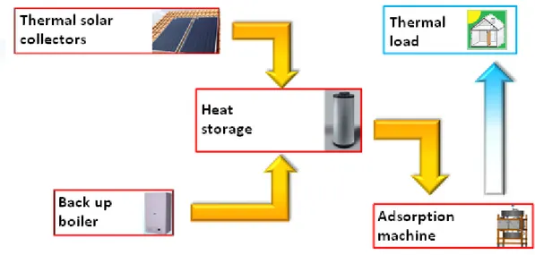
3.1. System overview and main components description
The system under investigation in this report (shown in Fig. 3-1) is made up of a thermally
19
storage tank is fed with water heated by a solar panel field and a back up boiler. The adsorption machine is connected to a dry-cooler transferring the heat rejection to the external environment. The chiller provides cold water for the fan-coil, which produces the cooling effect.
Fig. 3-1System plant layout.
The system dynamic model was built in order to find the optimum values for solar panel field (type, surface and technical specification) and for heat storage volume.
Solar collector used to collect heat for solar cooling application or domestic hot water production can be divided in two main groups: flat plate and evacuated tube collectors.
Flat plate collectors (see Fig. 3-2) consist of an insulated metal box (glass wool is mainly used) to minimize heat losses, a dark-colored absorber plate, to absorb most of the solar radiation and a low iron content glass cover, to obtain high transparency to solar radiation. Solar radiation is absorbed by the plate and transferred to the fluid that circulates through tubes, which are placed between the absorber plate and the glass cover.
20
Fig. 3-2 Flat plate collector.
Evacuated tube collectors (Fig. 3-3) consist of evacuated borosilicate glass tubes which heat up solar absorbers and, ultimately, solar working fluid (water or propylene glycol). The vacuum within the evacuated tubes reduces convection and conduction heat losses, allowing them to reach considerably higher temperatures than flat-plate collectors.
Fig. 3-3 Evacuated tube collector.
The main differences between solar plate and evacuated tube collectors are as follows:
- Cost: evacuated tube collectors are more expensive than flat plate collectors due to their
high tech level
- Required temperature: evacuated tube collectors can achieve higher temperature than
flat plate
- Available surface for installation: evacuated tube collector requires less surface than flat plate to meet the system’s power requirements.
21
Fig. 3-4 Vertical heat storage tank connection.
The hot water stream feeding the adsorption chiller flows inside the storage leaving from top and entering from bottom. The lower heat exchanger is connected to the solar panel field, while through the higher one flows the water heated by the auxiliary boiler to prevent from using auxiliary power to heat all the storage volume.
3.2. Dynamic model and simulations
The model was built using TRNSYS software. TRNSYS is a simulation program mainly used in the fields of renewable energy engineering and building simulation for passive as well as active solar design. TRNSYS is a commercial software package developed at the University of Wisconsin.
The components of the model are called “types”. The software comes with a wide set of types used in this kind of installation: solar collector (flat plate and evacuated tubes), heat storage tank, chiller and adsorption machine. The software also allows user to create custom types when needed by using FORTRAN subroutines.
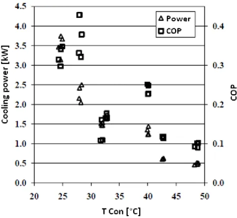
The adsorption machine and the type able to simulate its behavior were developed by the CNR-ITAE in Messina on the basis of experimental data, obtained by ITAE [3] and shown in Fig. 3-5 and Fig. 3-6:
22
Fig. 3-5 Power and COP referred to the temperature at condenser.
23
The type operates on input data (see Fig. 3-7) using parametric functions, which are obtained by linear interpolation of experimental measurements.
INPUT
• Temperature: condenser, evaporator and adsorbent beds • Flow rate: condenser,
evaporator and adsorbent beds
OUTPUT
• Temperature: condenser, evaporator and adsorbent beds • Flow rate: condenser,
evaporator and adsorbent beds • Power: heating, cooling,
chilling • COP
Fig. 3-7 Chiller type input and output
The solar cooling system considered in this study is intended to provide comfort conditions in an office room located in Messina (Sicily) in summer. Table 3-1 summarizes the main features of the design.
Room description
West wall surface 7.5 m2
East wall surface 7.5 m2
Nord wall surface 12 m2
South wall surface 12 m2
West window surface 1 m2
East window surface 1 m2
Nord window surface 1 m2
Room surface 10 m2 Room Volume 30 m3 Internal load Occupancy (time) 2 (8-18) Personal computer 2 Artificial lighting 10 W/m2
24
The simulations for the determination of the thermal load were performed with TRNSYS The typical input data scheme is shown in Fig. 3-8:
Fig. 3-8 Zone input panel
Results for the warmest summer week are shown in Fig. 3-9. Set point conditions were as follows: 26 °C and 50% relative humidity.
25
Fig. 3-9 Room thermal loads.
Since the peak load is considerably below 2 kW the adsorption chiller would be capable to meet system requirements.
The system model has been developed with TRNSYS Studio with the components (types) summarized below. They all came with TRNSYS software with the exception of the adsorption chiller built by CRN – ITAE.
- Type 109, Data Reader and Radiation Processor. This component serves the main
purpose of reading weather data at regular time intervals from a data file, converting it to a desired system of units and processing the solar radiation data to obtain tilted surface radiation and angle of incidence for an arbitrary number of surfaces. In this mode, Type 109 reads a weather data file in the standard TMY2 format. The TMY2 format is used by the National Solar Radiation Data Base (USA) but TMY2 files can be generated from many programs, such as Meteonorm.
- Type 538, Evacuated Tube Solar Collector. This component models the thermal
performance of a evacuated tube solar collector. The solar collector array may consist of collectors connected in series and in parallel. The thermal performance of the collector
26
array is determined by the number of modules in series and the characteristics of each module.
- Type 540, Flat Plate Solar Collector. This component models the thermal performance
of a flat-plate solar collector. The solar collector array may consist of collectors connected in series and in parallel. The thermal performance of the collector array is determined by the number of modules in series and the characteristics of each module. The user has to provide results from standard tests of collector efficiency versus a ratio of fluid average temperature minus ambient temperature to solar radiation.
- Type 700, Boiler. This component models the boiler (auxiliary heater). This model will
attempt to meet the user-specified outlet temperature taking into account the boiler efficiency and the combustion efficiency, which have to be defined by the user.
- Type 60, Vertical Storage Tank. This component models a stratified liquid storage tank.
It includes numerous features such as allowing for multiple heat exchangers within the tank and allowing for unmatched numbers of inlet and outlet flows. Users may define between 0 and 3 (inclusive) internal heat exchangers.
- Type 508, Cooling Coil Using Bypass Fraction Approach. The cooling coil is modeled
using a bypass approach in which the user specifies a fraction of the air stream that bypasses the coil. The remainder of the air stream is assumed to exit the coil at the average temperature of the fluid in the coil and at saturated conditions. The model is alternatively able to internally bypass fluid around the coil so as to maintain the outlet air dry bulb temperature above a user specified minimum.
- Type 753, Heating Coil Using Bypass Fraction Approach. This component models a
simple heating coil where the air is heated as it passes across a coil containing a hotter fluid (typically water). It uses the bypass fraction approach for heating coils to solve for the outlet air and water conditions. This model has been used to simulate how the dry cooler behaves.
- Type 56, Multi-Zone Building. This component models the thermal behavior of the
building previously generated by running the preprocessor program TRNBuild.
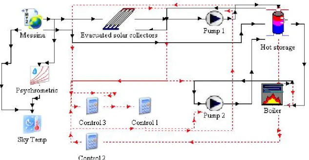
Types simulating pumps, flow diverters, flow mixers and fans were also used to obtain the whole system layout, as shown in Fig. 3-10.
27
Fig. 3-10 TRNSYS system layout.
As appears in Fig. 3-10, the system is split in three subsystem referring to the hot side, the cold side and the load. There are also components that display the system output data or controlling the on/off timing. The three subsystems are shown and described below.
Fig. 3-11 Hot side subsystem.
Fig. 3-11 shows the “hot side” subsystem, whose components provide hot water for the adsorption machine. It is possible to recognize the solar collectors and the boiler connected to the heat storage. The two pumps, controlled by additional types, make the fluid flow go across the storage heat exchangers.
28
Fig. 3-12 Cold side subsystem.
Fig. 3-12 shows the “cold side” subsystem. There are two types simulating two adsorption machines in series, in order to match all the cooling load. Simulation results show that the second chiller provides only 1% of the total cooling power, and is in idle for the majority of the time. Two heating coils simulate the dry cooler, which removes the machines thermal waste, while the cooling coil simulates the fan coil, which reduces the room air temperature.
Fig. 3-13 Load subsystem.
Fig. 3-13 shows the “load subsystem”. The room type was created, as described above, with the TRNBUILD feature. Two additional types are used to control infiltration and air change flow rates during the course of the day.
29
The collectors and boiler pumps control system was made up in order to achieve the highest efficiency. The main points taken into account while developing the control were:
- The office is occupied by the two persons from 8.00 a.m. to 6.00 p.m., so the adsorption
machine would work only during this time.
- The pump connecting the solar collector to the heat storage makes the fluid flow
circulate only if the outlet collector fluid temperature is higher than the stored water temperature. This is to avoid stored water being cooled by the collector fluid flow.
- The boiler is turned on when the heat storage temperature falls below 80 °C, to prevent
the adsorption machine from working with water at low temperature.
- The whole system is off during night, when no solar radiation can be gathered by solar
collectors.
3.3. Simulation results
The TRNSYS model has been used to perform different parametric analysis. The simulation time starts on June the 15th and ends on September the 15th. Simulations were run to find the optimum for the system referring to:
- Solar collectors tilt angle
- Heat storage tank volume
- Total collectors surface.
The technical specification for the solar collectors, heat storages and boiler types were taken from real components available in the market. The flat plate and evacuated tube collectors are from the same manufacturer, and the same is for three different heat storage models.
30
Fig. 3-14 Solar collector chosen for the simulation.
Fig. 3-15, 16 and 17 show the technical specification of the three heat storage tanks chosen.
31
Fig. 3-15 300 dm3storage.
32
Fig. 3-17 750 dm3storage.
To evaluate and compare the system performance two different parameters were taken into account:
• The Solar Fraction, which is defined as the ratio of the solar power to the total thermal load which, in turn, is the sum of the thermal power provided to the system by both the solar collectors and the boiler:
boiler coll coll Q Q Q SF & & & + = (3.1) Where:
SF is the Solar Fraction
coll
Q& is the thermal power provided by the solar collectors
boil
33
• The Primary Energy Ratio, which is defined as the ratio of the enthalpy difference between the inlet flow rate air and room inside air to the total Primary Energy provided form outside to the whole system (gas boiler and auxiliary devices):
37 . 0 / aux gas P Q h PER + = & (3.2) Where:
PER is the Primary Energy Ratio
h is the enthalpy difference between inlet flow rate and room air gas
Q& is the boiler Primary Energy consumption aux
P is the auxiliary devices electrical consumption, which is converted to Primary
Energy consumption by means of the Italian electrical power production efficiency (0,37)
The auxiliary devices consumption data were taken from the manufacturer technical specifications, and were assumed to be equal to 800 W.
The first set of simulations investigates about the optimal solar field tilt angle. The solar collectors field is due to south (only the tilt angle was changing).
Fig. 3-18 refers to simulations for evacuated tube collectors, while Fig. 3-19 refers to simulation related to flat plate collectors. Both of them show how the SF reacts to the tilt angle.
34
Fig. 3-18 SF vs. Evacuated tube collector field tilt angle.
35
Fig. 3-18 shows that the evacuated tube collectors allow to achieve high values of SF into a wide range of tilt angle values. This is due to the cylindrical concentrating surfaces, located inside the collector, which can gather energy from the solar radiation even if it is not perpendicular to the plate surface. On the other hand, flat plate collectors work at their best only in a little range of tilt angle, because they absorb the solar radiation only if it is perpendicular to the plate surface (see Fig. 3-19).
Fig. 3-20 and 21 show the results obtained in terms of PER. They refer to the same set of simulations done for the SF analysis.
36
Fig. 3-21 PER vs. Flat plate tube collector field tilt angle.
These graphs show that even from the PER point of view the evacuated tube collector field works better than the flat plate tube collector field, being less influenced by the tilt angle. Taking into account these results, the tilt angle for all of the further simulations performed has been set equal to 20° for both the evacuated and the flat plate collectors fields.
A second set of simulations was aimed at finding the best values for both the total solar collectors area and the volume of heat storage. Simulations related to the optimum for the solar collectors area per unit of nominal solar power installed (A) were performed according to the formula provided by H. M. Henning [4].
coll
COP G
A= 1 (3.3)
The average solar radiation value (G) has been set equal to 0.8 kW/m2and the machine COP
can be assumed equal to 0.35. For the evacuated solar collectors, whose thermal efficiency ( coll) is equal to 0.55, the result is 6.5 m2/kW, while, for the flat plate collectors, whose
37
thermal efficiency is equal to 0.4, the result is 18.5 m2/kW. As the system has to be capable of providing a cooling peak power equal to 2 kW, simulations have been run considering a
maximum area of 13 m2 for the evacuated tube collectors and 19 m2 for the flat plate
collectors.
Results are shown in Fig. 3-22:
Fig. 3-22 Solar Fraction vs. Evacuated solar collectors area for different values of heat storage volume.
Fig. 3-22 shows how the SF value changes using different values for the evacuated solar collectors area and for the heat storage volume. SF does not seem to be affected by changing in the heat storage and it reaches a very high level (95 %) with just 8.5 m2of solar collectors.
38
Fig. 3-23 Solar Fraction vs. Flat plate solar collectors area for different values of heat storage volume.
Fig. 3-23 shows how the SF depends on the total flat plate collectors area and on the heat storage volume. Using flat plate collectors, high level of SF can be achieved only with high surface of solar panels and the heat storage has a relevant impact on the system performance. This happens because the flat plate collectors work at their best only a few hours a day and the system has to be able to store the thermal power needed during the low efficiency hours.
The highest SF value (0,90 %) can be reached by using 18.5 m2 of flat plate solar collectors
and a heat storage volume equal to 0.75 m3.
39
Fig. 3-24 PER vs. Evacuated solar collectors area for different values of heat storage volume.
0 0.05 0.1 0.15 0.2 0.25 0.3 0.35 0.4 0.45 0.5 0.55 0.6 0.65 0.7 0.75 4 6 8 10 12 14 16 18 P E R
Solar collectors area [m2]
Heat storage: 0.3 m^3 Heat storage: 0.5 m^3 Heat storage: 0.75 m^3
40
PER results are very similar to SF results as they depend on the same conditions. Using evacuated tube allows to gather more solar thermal energy than using flat plate collectors and make the system less depending on the heat storage volume. Using evacuated solar collectors also allows to reach higher SF values than using flat plate collectors with lower collecting area.
In conclusion the solar cooling system was finally designed withn the following specifications:
• series of 4 evacuated tube solar collectors; • solar collectors area equal to 8.44 m2;
• gross solar collectors area equal to 11.52 m2; • solar field tilt angle equal to 20°;
• heat storage volume equal to 0.3 m2;
The simulation performed according to these values ensures that this system can grant the required comfort level to the room inhabitants, even during the warmest observed summer week. The week starts on July the 17th and ends on 23th. Fig. 3-26 shows that the inside temperature would not rise over 26 °C, while the outside temperature reaches 34 °C.
41
Fig. 3-26 Inside and outside temperature during the warmest summer week.
3.4. Energy analysis and plant sizing
Since the system is able to control the air temperature, but it cannot operate any regulation on air relative humidity, only the sensible cooling load will be taken into account for a deeper thermal analysis.
3.4.1. Thermal loads
The total thermal load (Qsens) is given by the sum of external (Qsens,est) and internal (Qsens,int) thermal loads. The result is provided by TRNSYS simulation.
kW Q
Q
Q&sens = &sens,est + &sens,int =1,4
Since the room is occupied by two persons, the system has to provide fresh air from outside according to the Italian regulation (Norma UNI 10339) the fresh air flow rate depends on people occupancy and is set to
pers h
m3
42
Outside fresh air enters at external temperature (tE = 30 °C) and, after an adiabatic mixing
with ambient air, its temperature decreases to 26 °C. The corresponding cooling load has to be taken into account:
s kg m kg pers h m mfresh 0.03 3600 1 22 , 1 2 40 3 3 = &
(
t t)
kW cp mQ&fresh = &fresh a E A 0.1
Where cpastands for air specific heat capacity
K kg kJ 004 , 1 The total sensible load is equal to:
kW Q
Q
Q&sens,tot = &sens + &fresh =1,5
Now it is possible to go on with the thermohygrometric analysis of the system.
3.4.2. Fan coil
The fan coil removes heat from the ambient air. The unit gets cold water at the temperature of 13 °C (tch,out) from the adsorption chiller. The cold water flow rate circulating through the cold piping system, which connects the fan coil to the cooling machine, is given by the energy balance on the component. The outlet water temperature is supposed to be 18 °C, so that the difference between fan coil water inlet and outlet ( tfc) is equal to 5 °C.
s kg m t cp m
Q&sens,tot = &w,fc w fc &w,fc 0,07
Where cpwstands for water specific heat capacity
K kg kJ 186 , 4
The air flow rate handled by the fan coil is known from its technical specification:
h m ma fc 3 , =600 &
Fan coil outlet air thermohygrometric conditions are:
kg g x kg kJ h C c m t c m t t I I pa fc a fc pw fc w A I 18.5 45.14 10.5 , , = ° = = = & &
43
3.4.3. Adsorption machine
The adsorption machine has to provide all the cooling power required for air conditioning. The thermal power (Qhot) needed to produce the cooling effect can be calculated on the basis of the estimated COP value.
kW COP Q Q senstot hot 5 , = & &
The chiller receives hot water from the storage at a temperature (Thot,in) of 85 °C. The hot water flow rate circulating through the hot piping system, which connects the adsorption chiller to the hot water storage, is given by the energy balance on the component. The outlet water temperature is supposed to be 80 °C, so that the difference between fan coil water inlet and outlet ( thot) is equal to 5 °C.
s kg m t cp m
Q&hot = &w,hot w hot &w,hot 0,24
The total thermal power entering the adsorption machine is the sum of Q&hot +Q&sens,tot kW
Q
Q&hot + &sens,tot =6,5
The same quantity leaves the adsorption machine moving towards the dry cooler
3.4.4. Dry cooler
Thermal waste production (Q&sens,tot +Q&hot) belonging to the adsorption machine is transferred to the environment by the dry cooler. The inlet water temperature (tdc_in) is 35 °C, the outlet water temperature (tdc_out) is 30 °C, so the temperature difference ( tdc) is equal to 5 °C. By means of the energy balance the dry cooler flow rate results equal to:
s kg t c Q Q m dc pw hot tot sens dc 0,31 , + = = & & &
The total power entering the dry cooler is the sum of thermal power belonging to the adsorption machine (Q&hot +Q&sens,tot) plus the required grid electrical power (Pel = 700 W).
kW P
Q
44
3.4.5. Thermal solar collectors and gas boiler
The optimum for thermal solar collector, according to dynamic simulation, is a 11,5 m2
evacuated tube field. The related SF value has been set to 80%:
8 , 0 = + = boiler coll coll Q Q Q SF
Thermal power provided by heating devices (solar collectors (Qcoll) and boiler (Qboiler)) are:
(
SF)
kW Q Q kW SF QQ&coll = &hot =4 &boiler = &hot 1 =1
Referring to the technical specification provided by the manufacturer, the solar collector circulating water flow rate (mcoll) is 0,08 kg/s. The water temperature difference ( tcoll) between collector inlet and outlet is:
C m cp Q t coll w coll coll = =12,1° & &
The solar collector energy efficiency is also provided by the manufacturer: % 8 , 54 = sc
The thermal power delivered with the incident solar radiation (Q&sun) is:
kW Q Q sc coll sun = =7,3 & &
The water flow rate circulating inside the boiler (m&boiler) can be calculated by means of the energy balance on the component. The temperature difference between water inlet and outlet ( tboiler) has been set to 5 °C
s kg t cp Q m boiler w boiler boiler = =0,05 & &
The thermal power provided by the fuel (Q&fuel),assuming boiler = 0,9, is
kW Q Q boiler fuel 1,1 9 , 0 = = & &
The thermal power produced by both solar collector and boiler is delivered to the heat storage tank by means of two heat exchangers. The temperature of the water, feeding the adsorption machine, inside the storage is equal to 85 °C.
45
3.4.6. Results of energy analysis
The global system thermal performance will be now calculated. Two different index will be
used: the COPglobal and the COPrnw. Both of them are ratios between thermal energy entering
into the system and the provided cooling effect but the former involves all the thermal energy (solar collector + boiler) while the latter (COPrnw) is calculated without taking into account the thermal energy gathered from the sun, which is a renewable energy source.
3 , 0 5 , 1 , , = + = = = coll boiler tot sens global boiler tot sens rnw Q Q Q COP Q Q COP & & & & &
Results are summarized in Table 3-2 Energy analysis resultswhile Fig. 3-27 provides a
graphic representation of the global energy balance.
Component Qin [W] Qout [W] Loss [W] Loss [%] Efficiency [%]
Solar collectors 7300 4000 3300 97 54,8 Boiler 1100 1000 100 3 90,0 Heat storage 5000 5000 0 0 100 Dry cooler 6500 + 700 7200 0 0 N.d. Adsorption machine 1500 6500 0 0 COP = 0,3 Fan coil 1500 1500 0 0 100 Total 3400 100
Table 3-2 Energy analysis results
The fan coil and the hot storage have efficiency index equal to maximum achievable (100%) and the boiler a very high one (90%). From a First Law point of view it seems that the main inefficiencies in the system belong to the adsorption machine and to the solar collector.
46
Fig. 3-27 Energy flow chart.
In the energy flow chart only two components are responsible of considerable losses (solar collector and dry cooler), while the others are apparently “ideal” (like the storage or the fan coil).
3.5. Exergy analysis
Now, the exergy analysis of the system will be carried out to point out the efficiency in exploiting the thermodynamic potential of energy sources referring to the final use. For each
SOLAR COLLECTORS Pel Pel 7300 W 1100 W 3300 W 4000 W 1000 W 100 W 5000 W 5000 W 1550 W 700 W 7250 W 6050 W 1500 W BOILER STORAGE CHILLER FAN COIL ROOM DRY COOLER 50 W
47
component the irreversibility production will be calculated as the difference between the entering and exiting exergy flows, as stated by the Gouy - Stodola Theorem. The ratio between the same values gives the index of exergy efficiency.
3.5.1. Solar collectors
The exergy flow entering into this component is provided by the solar radiation and can be calculated by using the eq. (2.9):
kW T T Q E plate E SC coll SUN in_ = 1 =1,69 &
where Tplate is the average collector temperature and SC is the collector energy efficiency.
The simulation results give Tplate = 393 K and SC = 0,55.
The inlet/outlet water flow rate exergy gain, which depends on the temperature difference, can be now calculated by using the eq. (2.18)
kg kJ e
kg kJ
ecoll_in =96,9 coll_out =106,6
The total exergy gain (Eout,coll) provided by the solar panel field is:
(
e e)
kWm
Eout,coll = &coll coll_out coll_in =0,77
The irreversibility production (Icoll) can be calculated as the difference between the inlet (Ein_sun) and the outlet (Eout,coll) exergy flow:
kW E
E
Icoll = in_SUN out,coll =0,92
The exergy efficiency index coll is (see eq.2.16)
% 5 , 45 _ , = = SUN in coll out coll E E 3.5.2. Boiler
The exergy flow rate entering the boiler can be calculated by means of the eq. (2.9) but now
the highest temperature is the flame temperature (TF = 1500 K) and the energy efficiency
index is BL = 0,9. kW T T Q E F E BL boiler BL in_ = 1 =0,89 &
48
The inlet/outlet water flow rate exergy gain, which depends on the temperature difference, can be now calculated by means of eq. (2.18).
kg kJ e
kg kJ
eboiler_in =91,4 coiler_out =96,9
The total exergy gain provided by the solar panel field is:
(
e e)
kWm
Eout,BL = &boiler boiler_out boiler_in =0,17
The irreversibility production (Iboiler) can be calculated as the difference between the inlet (Ein_BL) and the outlet (Eout_BL) exergy flow:
kW E
E
Iboiler = in_BL out_BL =0,72
The exergy efficiency index boier is see (2.16):
% 1 , 19 _ _ = = BL in BL out boiler E E 3.5.3. Heat storage
The heat storage does not play any role in the energy balance (from a First Principle point of view) under the steady state hypothesis: the entering energy flow equals the exiting one. But from a Second Principle point of view the thermal energy storing leads to inefficiency production related to the heat exchange.
The entering exergy flow (Ein,store) rate can be calculated as the sum of the exergy flows exiting from the solar panel field (Eout,coll) and from the boiler (Eout,BL):
kW E
E
Ein,store = out,coll + out,BL =0,94
The exiting exergy flow rate feeds the adsorption machine and is related to the difference between the inlet and outlet chiller hot water temperature (Thot,in = 358 K e Thot,out = 353 K).
kg kJ e
kg kJ
eads_in =90 ads_out =87
The heat storage outlet exergy flow rate (Eout,store) is:
(
e e)
Wm
Eout,store = &w,hot ads_in ads_out =748
The irreversibility production (Istore) is: W
E E
Istore = out,store in,store =197
49 % 6 , 79 , , = = acc in acc out acc E E
There isn’t any transformation taking place inside the heat storage. All the irreversibility production is given by the heat transfer (that implies temperature difference) between the fluid circulating through the two heat exchangers and the hot water stored.
3.5.4. Dry cooler
The dry cooler transfers the heat rejection coming from the adsorption machine condenser to the external environment. The specific exergy flow exiting from this component can be calculated knowing inlet and outlet temperature (Tdc_in = 308 K, Tdc_out = 303 K):
kg kJ e kg kJ edc_in =71,6 dc_out =71,4 The total oulet exergy flow is:
(
e e)
Wm
Eout,dc = &w,dc dc_in dc_out =54
This component uses electrical energy, which is pure exergy, to operate; so the total inlet exergy flow equals the electrical power consumption:
kW P
Ein_dc = el,dc =0,7
The irreversibility production is: W E
E
Idc = out,dc in,dc =646
The dry cooler exergy efficiency index ( dc) is:
% 7 , 7 , , = = dc in dc out dc E E
The irreversibility production belonging to this component is very high due to the high quantity of electrical energy (= pure exergy) needed to operate.
3.5.5. Fan coil
The Fan Coil operates the heat exchange between the cold water flow rate m&w,fc, which has
been cooled down at the temperature tfc,in = 13 °C by the adsorption machine, and the room
50
fan coil is tfc,out = 18°C, and this temperature gap is one of the two exergy flows which fuel this component. The other one is the electric power needed to operate (Pel,fc = 50 W).
The inlet and outlet water specific exergy contents are:
kg kJ e kg kJ efc_in =73,4 fc_out =72,4 The total inlet exergy flow is:
(
e e)
P Wm
Ein_FC = &w,fc fc_in fc_out + el,fc =76+50=126
The outlet exergy flow can be calculated taking into account the fan coil inlet and outlet air temperature difference and the air flow rate. These data allow to calculate the sensible thermal load covered, which is the exergy flow rate exiting from the fan coil. The room air and the fan
coil outlet air specific exergy contents can be calculated by using the eq. (2.17) referring to
these quantities:
Room air temperaure (tA) = 26 °C, fan coil outlet air temperature (tI) = 17,4 °C, Room air and fan coil outlet air humidity ratio (xA= xI) = 10,5 g/kg.
kg kJ e kg kJ eA =0,5 I =0,87
(
e e)
W m Eout_FC = &a,fc I A =74 Where:• eAis the room air specific exergy content;
• eI is the fan coil outlet air specific exergy content; • m&a,fc is the air flow rate;
• Eout_FC is the fan coil outlet exergy flow rate. The irreversibility production is:
W E
E
IFC = in_FC out_FC =52
The fan coil exergy efficiency index ( fc) is:
% 7 , 58 _ _ = = FC in FC out Coil Fan E E