Models and Systems for the Control of Two-Phase Processes in Microfluidics

(1)

Fabiana Cairone

Models and Systems for the

control of two-phase processes

in microfluidics

Doctor of Philosophy in Ingegneria dei Sistemi, Energetica,

Informatica e delle Telecomunicazioni

UNIVERSITÀ DEGLI STUDI DI CATANIA

(2)

Dipartimento di Ingegneria Elettrica Elettronica e Informatica

Doctor of Philosophy in Ingegneria dei Sistemi,

Energetica, Informatica e delle Telecomunicazioni

Models and Systems for the control

of two-phase processes in

microfluidics

Candidato: Fabiana Cairone

Relatore: Chiar.ma Prof. Ing. Maide Bucolo

(3)

Abstract

The strong point of the microfluidics is the ability to miniaturize and integrate one or several laboratory functions on the same device, to have a portable and user-friendly instrument. Most applications require accurate measures and con-trol within the microfluidic channels. In this thesis, the optical techniques were adopted to monitor, sensing and control the processes, leading to the research area of optofluidics that are based on the integration of fluidics and optics. To reduce the cost to develop these devices, the 3D Printing technology based on the Poly(dimethyl-siloxane) (PDMS) is proposed. All these aspects were addressed considering the two-phase flow (named slug) generated by the interaction of two immiscible fluids, a very common condition in bio-chemical applications. The methodological aspects were discussed in the first part of the thesis, starting from the extraction of parameters for the flow characterization, to their use for the flows real-time modelling and control schemes development; the second part in-vestigates aspects faced for the realization of micro-optical flow detector by using the 3D Printing technology.

(6)

Introduction

Microfluidics is a novel and promising scientific field research whose progresses are aimed to the development of the Lab-On-Chip (LOC) systems. The strong point is the ability to miniaturize and integrate one or several laboratory functions on the same device, which thus becomes a portable and user-friendly instrument. The progresses made in the recent years have led to the realization and diver-sification of devices for chemical and biological analysis and biomedical applica-tions [1, 2]. The advantage that could arise from the introduction on the market of disposable low cost diagnosis tools, as the Point-of-care (PoC) devices, can be evinced by their demanding and increasing request in medical and pharmaceutical sectors [3–5].

At the moment, the results presented in literature are strictly related to specific experimental conditions, so far from a well-established framework that can drive to the flow control [6]. Recently, some case studies have been presented in lit-erature using a System-on-a-Chip (SoC) approach that embeds model predictive control strategies [7–9]. The SoC offers an high control level and modularity but its functionalities are strongly dependent from the integrated control logic and the knowledge of process model [10]. The need of a process model represents an important bottleneck for a widespread diffusion of its use in PoC applications. Most of these applications require accurate measures and control within the mi-crofluidic channels [11]. The optical techniques were adopted to monitor, sensing and control the processes [1, 12], leading to the research area of the optofluidics that are based on the integration of optics and fluidics [13].

The traditional methods to investigate the flows are based on the acquisition by using a fast CCD camera or a micro-PIV system [14]. Both instrumentation are noninvasive and allow to have detailed and accurate information about the

(7)

mi-Introduction v

crofluidic process, but with the drawbacks related to the cost [15].

To reduce the cost to develop the device and, at the same time, to have the optics and fluidics parts integrate in the same device, the 3D printing technology based on the Poly(dimethyl-siloxane) (PDMS) is proposed.

All these aspects have been addressed considering a two-phase flow (named slug flow) generated by the interaction of two immiscible fluids in a micro-channel, a very common condition in many bio-chemical applications. This thesis consists in two parts:

• Part I is divided in four chapters and deals with the methodologically aspects in the real-time modelling and the control of the slug flows;

• The Part II is divided in two chapters and presents the aspects faced for the realization of a micro-optical flow detector by using the 3D printing technology, as proposed low cost solution.

(8)

Part I

SLUG FLOWS IN

MICROFLUIDICS

(9)

Introduction

The two-phase flow identification and control is one of the main open issue in the construction of highly complex microsystems, where fluids can circulate in a controlled manner performing a large number of tasks in a maze of micro-channels. Moreover, it is important that it can be easily adaptable in different operative con-ditions and able to guarantee the process reproducibility and reliability [16]. Interfaces between the two fluids adopt elaborate forms, and the classification of regimes (identified as bubble, slug or plug, annular, churn and wispy annular) can sometimes lead to inextricable phase diagrams, where many regimes are mixed up [17].

The two-phase slug flow considered was generated by the mixing of two upstreams (gas - liquid). When at the same time two streams of fluid are co-injected in a curved micro-channel, stretching and folding of segmented fluid are possible. These nonlinear features recognized in two-phase flows are highlighted in the phenom-ena named as chaotic advection that was introduced as responsible for the fast mixing time of multiple reagents inside isolated plugs (slugs) in winding micro-channels [18–20]. The combined effect of the curved geometry and the channel width in the range [100 µm − 1 mm], referred as meso-scale in Ribatski et al. [21], leads from one side to the increase of the process complexity and the difficult on the processes control, and to the other side in the speeding up the flow and mixing up the different phases.

In the chapter one the research of a trade-off between these conditions drove the systematic experimental study on the slug flow patterns generation, in terms of length and frequency of the slugs, in a straight and serpentine micro-channels. The attention was focused on three issues: how the curves in the geometry affect the slug flow displacement, the role played by the input flow rates in the slug flow

(10)

3

characterization and how the flow changes in different channel positions.

Three methods are widely used in channel with width in the order of cm for the characterization of length and frequency of the bubbles: the slugs frequency pre-diction methods with correlation [22], mechanistic model [23] and the probabilistic approach [24]. The measures necessary for the application of these methods require detection systems that can be considered invasive and complex for micro-channels and reducing the possibility of their use in this context.

Starting from the first works of Triplett et al. [25,26], a wide literature is available dealing with the two-phase processes in micro-channels with width in the range [1 − 6] mm, as it can be evidenced in the review of Serizawa et al. [6]. Despite of that the biphasic flows in microsystem with a channel width less than 1 mm is still not well documented. The studies presented in literature mainly focus on two-phase flow characterization for specific application as the design heat ex-changer [21], the microevaporator [27] and the micro-reactor [28], but far from a well-established framework that could drive to the flow identification and control in a general condition. In the major examples presented in literature the study of segmented flows through signal analysis is performed by the pressure transduc-tion: flow regime [29, 30], pressure or velocity fluctuations [31–33], residence time distribution and slug displacement [34]. In comparison to that, the optic trans-duction [35] does not interfere with the process and offers significant advantages considering the small channel width: an easy adaptation for the simultaneous ac-quisition in different test positions [36] and the easy integration of optical sensors with the microfluidic chips [37, 38].

The most common way to optically monitor the process and collect information for the flow regime classification is by a continuous 2-D monitoring using fast CCD camera or µPIV system [14]. In both case, it is possible to obtain a detailed and precise information but with the drawbacks related to a costly and bulky equipment. The monitoring setups proposed in the development of this work were simplified to reduce the cost of the equipment to be used and make easier the op-tical components miniaturization. The opop-tical information was post-processed for the flow classification and characterization both in time and in frequency domains. In chapters two and three, the experimental results presented in chapter one for the flows characterization have been used for the development of data-driven

(11)

mod-4

els suitable for real-time tracking of the flow. From a theoretical point of view, the computational modelling of fluidic processes is based on the Navier-Stokes equa-tion (NS). If the Reynolds number (Re) is smaller than one, it is possible a model simplification assuming the linearization of the process based on the hypothesis that the slugs have a constant velocity and no dynamical interaction among each others. On the other hand, having more interacting fluids and Re > 10, no sim-plification is possible and the mathematical computational efforts increase. Generally, the models of multi-phase microfluidics systems are obtained by Com-putational Fluid Dynamics (CFD) [39]. Even so, the complexity of CFD, due to the high computation level and the not accessible analytical solution, can not make them suitable for on-chip applications.

To have useful information about the investigated processes and to predict the model that represents the process itself, the data-driven approach can be applied. These techniques use a collection of data to identify complex systems, which can-not be easily understood, analyzed and modelled [40]. The approach proposed is based on data-driven models for the identification of microfluidic processes easy adaptable for an on-line process control.

In particular, two methods are proposed: the first is based on nonlinear systems synchronization theory [41] and the second method is based on the class of Non-Linear Autoregressive with eXogen input (NARX) models [42] implemented by both the neural networks (NN) [43] and the wavelet networks (WN) [44] nonlinear mapping.

An example of unidirectional synchronization used for the time series identifica-tion is in Fortuna et al. [45] in which the experimental time series is assumed as a generic state variable of an unknown system and this information used to drive a second system with a known model and undefined parameters. On this purpose as known system was considered the Chua’s oscillator [46] due to dynamics diver-sification at the parameters change and, an iterative procedure based on Genetic Algorithm (GA) was used [47] to achieve the synchronization of the two systems by the parameters tuning. The models led to the successful identification of the slugs tracking and to quantify the slug’s velocity being correlated with the mean of the slug inter-distance.

(12)

5

slug flow. Based on the control system theory definition, the microfluidic two-phase processes can be considered in the class of the two inputs and single output nonlinear dynamical systems [15, 48]. The control action on the microfluidic pro-cess can be obtained passively or actively. A passive control can be implemented to generate a specific flow pattern, exploiting the geometrical properties of the micro-channel and the physical properties of the fluids involved in the process, such as the hydrophobicity or the surface tension between the fluids and the walls of the channels. This approach does not require additional energy sources and does not increase the complexity and the cost of the external equipment. On the other hand, the active control allows to have a desired flow pattern manipulating, in a precise and quick way, small amounts of fluids flowing in the micro-channel. Examples of active control are based on mechanical pumping [49, 50], pneumatic pressure [51] or magnetic field [52]. The active control is more robust than the passive and provides a high level of flexibility in the control of droplet size and frequency. Both the passive and active techniques often are developed based on a specific process issue and embedded on-chip, so they are not easily extended in a different context and needs. The proposed solution overcomes these drawbacks, it is on the class of active control but, instead of using an electro-mechanical control system takes the advantage of the optical monitoring and the on-line signal pro-cessing to develop a general purpose data-driven approach to control the droplet flow in the micro-channel. Starting from the optical process monitoring and the analysis procedure for the flow characterization, a control parameter was identified and the open loop and closed loop control system implemented.

(13)

Chapter 1 Slug flows in micro-channels

1.1 Theoretical background

Two-phase flows are distributed into several distinct flow patterns depending on the liquid and gas flow rates and fluid and channel properties. Five main flow regimes were observed in the partially wetting square micro-channels: bubbly, wedging, slug, annular and dry flows. Specifically, in the slug flows on which we focus the attention, the bubbles have approximately the same diameter of the tube and their size is far longer than the channel height. The length of the bubbles can vary considerably. The nose of the bubble has a characteristic hemispherical cap and the gas in the bubbles is separated from the tube wall by a thin film of liquid. The liquid flow is contained mostly in the liquid slugs which separate successive gas bubbles [53].

In general, the two-phase processes are modelled by a nonlinear system of par-tial differenpar-tial equations combining: the Navier-Stokes (NS) equation, describing the transport of momentum, the continuity equation and an inter facial tracking method [54].

The system of equations governing the process of two incompressible and immis-cible phases in terms of the velocity (v) follows:

(14)

Slug flows in micro-channels 7 ρ(∂v ∂t + v · ∇v) = −∇P + ρg + ∇µ(∇v + (∇v) T ) + G∇φ (1.2) ∂φ ∂t + v · ∇φ = χε 2 ∇2G (1.3) G = 3εσ 2√2(−∇ 2_{φ +} φ(φ2 − 1) ε2 ) (1.4)

The reported system consists of the continuity equation (eq. 1.1), the NS equation (eq. 1.2) and the Cahn-Hilliard equation (eq. 1.3) to model the interface dynamics by the phase field variable (φ). The chemical potential G expresses the rate of change of free energy (eq. 1.4). The forces on the right-hand side of NS equation are due to the pressure tensor (∇P ), the gravity (g) and the surface tension (G∇φ).

ε is the capillary width controlling the thickness of the diffusive interface, χ is the

mobility tuning parameter, and σ is the surface tension coefficient between the two phases.

The fluid interface corresponds to the region where the phase field variable φ is in the range ] − 1, +1[ and takes the values of ±1 in the two bulk phases (φ = −1 for the carrier fluid and φ = 1 for the dispersed phase). The density (ρ) and viscosity (µ) depend on the phase field as in the following equations:

ρ = 1 − φ 2 ρ1+ 1 + φ 2 ρ2 (1.5) µ = 1 − φ 2 µ1+ 1 + φ 2 µ2 (1.6)

In the multi-phase flow the evolution of the phase field variable governed by the Cahn-Hilliard equation involves a 4th-order derivative with respect to φ, this makes its treatment more complex than the NS equation in the single phase flow which involve only 2nd-order derivatives.

Considering the role of the input flows in the droplet formation and the flow patterns regime, four dimensionless numbers, reported in equations 1.7-1.10, have been widely investigated in microfluidics [55]: the Reynolds number (Re), the Capillary number (Ca), the Dean number (De) and the Air Fraction (AF ).

(15)

Slug flows in micro-channels 8 Re = < ρ >< v > D < µ > (1.7) Ca = < µ >< v > σ (1.8) De = Re ó D 2Rc (1.9) AF = Vair Vair+ Vwater (1.10) Dealing with two-phase flow, the < v >, < µ > and < ρ > are, respectively, the average velocity related to the two input flow rates and the mean of the fluid densities and viscosities. D is the characteristic dimension of the channel, Rc is

the radius of curvature of the path channel and σ is the surface tension coefficient between the two phases. The Vair and Vwater are the volumetric input flow rates

of the two fluids.

The Reynolds number (Re), expressed by the ratio between the inertial and the viscous terms in the NS equation, is an indicator of flow nonlinearity. At the transition between laminar and turbulent flow it is of the order 103_{, while for}

Re ≪ 1 the flow is dominated by the viscous stress, and the pressure gradient and

the inertial effect are negligible. The Capillary Number (Ca) captures the relative importance of viscous force to surface tension. This is a key aspect in two-phase flows for the droplet formation, since they are largely dominated by the interfacial effects. A value of Ca ≪ 10−2 _{leads to the droplet formation.}

1.2 Experimental setup

The global system used is schematized in Figure 1.1. It allows to generate the microfluidic process and to acquire the light intensity variations by means of a photodiode based circuit and a standard CCD camera, simultaneously. For the generation of microfluidic processes is extremely important the actuation system used to pump the flow and, the geometry and material of chip. These two choices determine a varity of process dynamics that can be generate.

(16)

Slug flows in micro-channels 9

Fig. 1.1. Schematic of global platform setup.

Many applications in the field of flow chemistry, micro-reaction equipment and mi-crofluidics depend on pulsation-free performance in the creation of fluid streams. This is because small flow rates in the nanoliter range require precision and smooth operation. The syringe pumps are widely used in microfluidic laboratories and they are based on a mechanical system actuated by an electric motor that push the sy-ringe at the selected rate. In this way it is possible to rely on highly accurate mechanical components, enabling continuous processes, improving product qual-ity, production flexibility and cost-effectiveness. In the experimental setup, two syringe pumps (Cetoni, NeMESYS) are used to inject fluids in the microfluidic chip through appropriate tubes. Thanks to the neMESYS UserInterface software, users can control these devices in order to change the flow rates. The microflu-idic chip (SMS0104, ThinXXS) selected to performing the experiments, is made in COC (Cyclo-Olefin Copolymer) which combines good optical properties with biocompatibility and good chemical resistance to most acids and bases. It offers different geometries and dimensions, as it is possible to see in Figure 1.2 and in Table 1.1. Each micro-channel in the chip presents a squared section.

The opto-mechanical setup (Thorlabs OTKB) provides two different ways to ac-quire information about the microfluidic process: photodiodes and CCD camera. Photodiode is a semiconductor device that converts light into current. They are made by a part to sense the luminous intensity. To acquire and analyze these signals, capture card is directly interfaced to the PC via acquisition board (PCI 6024-E, National Instrument).

(17)

Tab. 1.1. Dimensions of the microchannels

Channel Length(mm) Width/Depth(µm) Internal Vol.(µl)

1 21 100 0.2

2 121 640 49.6

3 66 320 6.8

4 50 320 5.1

5 16 320 1.6

Fig. 1.2. Microfluidic chip with different geometries and dimensions.

The user interface of the card is BNC 2110 with I/O analogic and digital and its maximum sampling rate is 200kS/s. The CCD image detector (DCU224, Thorlabs) allows capturing the image from light beams and to reproduce it on the computer screen through a dedicated software.

Three functional modules constitute the global platform setup:

• A light source focusing module composed by the white light source, the dichroic mirror and the condenser lens;

• A detection and actuation optic module constituted by the objective lens and the mirror;

• A sample stage and holder module made up by a sample stage which provides 3-axis (X, Y and Z) translation of the microfluidic chip.

In the first module, the light source is focused and applied at the sample (for ex-ample the microfluidic chip). The emitted light is split through a dichroic mirror (FM01, Thorlabs) that reflects 980 nm laser beam (trapping source) in one side

(18)

(a) (b)

Fig. 1.3. Pictures of the optical (a) setup − 1 used in the experimental set − 1/3; (b)

setup − 2 used in the experimental set − 2.

in the vertical axis and in the other side toward a black plastic end cap. Then it arrives at the condenser lens that condensates toward the objective lens in order to illuminate the sample in case of detection, while it is used to collimate the beam after the optical trap in case of actuation.

Detection and actuation optic module contains an objective lens and XY translat-ing lens mount (HPT1, Thorlabs), that allows to move the objective towards the sample, in such a way the working distances were respected.

The chip management module consists of a microscope slide holder mounted to a 3-axis (X, Y, and Z) translation stage (MAX301, Thorlabs) that is mounted on a 1-axis long travel translation stage (LNR50D, Thorlabs) and to a translating breadboard (TBB0606, Thorlabs).

Two optical setups were realized, labelled as setup − 1 and setup − 2. Both allow a simultaneous acquisition of light intensity variations, by means of a photodiode based circuit and a standard CCD (used with frame rate of 15 FPS). The setup−2 is an evolution of the setup − 1. In Figure 1.3 (a) and (b) two pictures show, respectively, the optical setup − 1 and the setup − 2. The equipment used in the two setups are detailed as follows: the halogen lamp (KL1500LCD, Olympus) used to backlit the process was substituted by an emitter Ultra Bright White LED (LEDWE-10, Thorlabs); the objective with 20X magnification was replaced with one of 10X; the pair of photodiodes (SLD-70BG2, Silonex) was changed with (SM05PD7A, Thorlabs) and the data acquisition board in setup−1 was PCI-6024E (National Instrument, used with a sample rate of 1 kHz) and in setup − 2 was PCI 6024-E (National Instrument, used with a sample rate of 4 kHz). The CCD active

(19)

area is 17 mm2 _{while each photodiode active area is equal to 1 mm}2 _{in the setup−1} and 6 mm2 _{in the setup − 2. The signals used for the flow investigation are those} acquired from the photodiode, giving an average information in their active area. A detailed description of the opto-mechanical system realized in the setup − 1 is in Bucolo et al. [56], while for the setup − 2 a modified version of the design presented in Appleyard et al. [57] was considered to have the contemporary signals and images acquisition. The signals were affected by frequency noise components related to the power supply and the illumination. A filtering procedure, that preserves the process dynamics, was implemented using a Butterworth low pass filter (fcut = 100 Hz and order N = 5), and two notch filters respectively at the

frequencies fcut = {50; 100}Hz with a quality factor Q = 3.

1.3 Experimental campaigns

The continuous slug flows were generated by pumping de-ionized water and air at the Y-junction of micro-channels. Three experimental sets were considered, named {set − 1, set − 2, set − 3}. The two syringe pumps were connected to the channel inlets and constant flow rates were imposed. The three geometries considered are shown, in details, in Figure 1.4: a straight channel with width

w = 320 µm and length l = 16 mm (labelled as G1), a serpentine with width w = 320 µm and length l = 50 mm (labelled as G2) and, a second serpentine

with width w = 640 µm and length l = 121 mm (labelled as G3). The curvature radius is, for the serpentine geometries, 1.28 mm. Introducing for {G2; G3} two analogous straight channels {G20, G30} with the same width and height, it was possible to deduce the hydraulic resistances {Rh1; Rh2, Rh3} [55]. The Rh2 is the greatest, three times bigger than that of Rh1 and two times bigger than that of Rh3.

In the experimental set −1, to evaluate the effect in the slug displacement induced by the curves, the process was monitored in an position located at a distance from the Y-junction of about 4mm in G1 (see Figure 1.4(a)) and, after 9 bends in G2 (see Figure 1.4(b)). In the experimental set − 2, the process was monitored in a position located at a distance of about 60 mm from the Y-junction, at the center of the straight part, tagged as point B in G3, to investigate on the flow pattern

(20)

(a) (b) (c)

Fig. 1.4. The micro-channel geometries considered. (a) The straight channel (G1);

(b) The serpentine (G2) with width w = 320 µm and length l = 50 mm; (c) The serpentine (G3) with w = 640 µm and length l = 121 mm.

after the slugs have experienced the mixing meander (see Figure 1.4(c)).

Additionally, in the experimental set − 3 the behaviour in the three positions in

G3 tagged as {A, B, C} was considered to highlight the changes in the slug flow

in relation to the closeness to the chip inlets and outlet (see Figure 1.4(c)). The setup − 2 was used for the acquisition in the experimental sets − 1/3 and the

setup − 1 for the experimental set − 2. Different apparatus were necessary for an

optimization of setup performance considering smaller channels, as in experimental

set − 1 and longer recording as in the experimental sets − 1/3.

The experimental set − 1 consists of 6 experiments. The attention was focused on the effects on the slug displacement due to the winding geometry. The two micro-channel geometries {G1; G2} were considered, and the two inputs flow rates were set equal (f = Vair = Vwater) varying in a set {0.1, 0.3, 0.5} ml/min.

Those values are lower respect to the one in the other experimental sets being the channel width smaller. This experimental set is marked in the input flow rates space reconstruction of Figure 1.5 with circles. The flow information was recorded in the area shown in Figure 1.4 (a) and (b) and each experiment recording lastes 240 s.

In the experimental set − 2, the micro-channel considered was G3 and a total of four experimental campaigns were designed. By these campaigns the role played

(21)

Fig. 1.5. The reconstruction of the input flow rates space (Vair, Vwater).

by the two inputs flow rates in the slug pattern generation in a serpentine micro-channel was investigated. Each campaign consists of 12 experiments in which one flow rate (Vair, Vwater) was fixed and respectively the others was varied. In the

campaigns − 1/2 the input flow rates were maintained below 1 ml/min (f ≤

1 ml/min), while they were one order of magnitude bigger (f ≥ 1 ml/min) in the campaigns − 3/4. The input flow rates space reconstruction is represented in Figure 1.5. In Table 1.2, the flow rate per campaign and the relative Air Fraction (AF ) are reported, and in Table 1.3 the ranges of the most significant dimensionless parameters in the process under investigation, as the Reynolds number (Re), the Capillary number (Ca) and the Dean number (De).

The Reynolds number values underline an increase of complexity in the flow for varying the input flow rates and, dealing with multiphase flows, it was computed using the average of the densities and input flow rates of the two fluids. For the

campaigns − 1/2 we are in a low Re number regime, while for campaigns − 3/4 we

are at the beginning of the inertial microfluidics regime [58]. The Capillary number values are in the range of [10−4_{; 10}−2_{], so always below the order of 10}−2 _that con-firms the theoretical expectancy of the droplet/slug formation. The Dean number expresses the relation between a secondary recirculation flow outside the slug due to the curves in the geometry taking into account the curvature radius [59]. The

(22)

Tab. 1.2. Air Fraction for the four experimental campaigns in set − 2. The flow rates

are in ml/min

AIR FRACTION (AF)

CAMPAIGN-1 Vair= 0.12 Vwater< 1 CAMPAIGN-3 Vair= 1.2 Vwater> 1 CAMPAIGN-2 Vair< 1 Vwater= 0.16 CAMPAIGN-4 Vair> 1 Vwater= 1.6 0.158 0.433 0.160 0.521 0.162 0.614 0.164 0.659 0.167 0.733 0.174 0.761 0.182 0.776 0.198 0.794 0.233 0.817 0.267 0.826 0.347 0.837 0.433 0.843

Tab. 1.3. Range of most significant dimensionless numbers for the four experimental

campaigns in set − 2. Re Ca (10−2) De CAMPAIGN-1 [0.93-2.54] [0.015-0.042] [0.65-1.8] CAMPAIGN-2 [0.93-3.35] [0.015-0.055] [0.65-1.8] CAMPAIGN-3 [9.26-25.4] [0.153-0.419] [6.55-17.96] CAMPAIGN-4 [9.26-33.53] [0.153-0.553] [6.55-23.71]

values in Table 1.3 underline a stronger influence at the increase of the input flow rate.

A variable pace was used varying Vwater and Vair based on flow visual inspection.

In Table 1.2, the air fraction (AF ) values associated to each experiment per cam-paign are reported and used for the results discussion. The air fraction values in

campaigns − 1/3 are equal, as those in campaigns − 2/4, but it is important to

notice that the input flow rates used in case of campaigns − 3/4 are one order greater than in campaigns − 1/2. Each experiment recording lasts 20 s; being the channel width greater and the process faster than in the experiment set − 1, a shorter time recording was sufficient to capture the flow dynamics.

The experimental set−3 consists of 9 experiments and the microchannel considered was G3. The aim of this investigation was the analysis of the changes in the slug patterns at different microchannel positions (or as well areas): close to the inlet point-A, at the center point-B and close to the outlet point-C. For each position a total of three experiments were considered assuming the input flow rates equal

(23)

Fig. 1.6. A CCD video frame sequence during an air slug passage in the investigation

area B of the micro-channel G3.

(f = Vair = Vwater) varying in the set {0.3, 1, 3} ml/min. The acquisition

procedure consisted in three steps: the optical system was centred in one of those points, then the two reference optical signals (micro-channel filled with water and filled with air) were recorded and, finally, the acquisitions for the three established flow rates began. This experiment set is marked with stars in the input flow rates space reconstruction of Figure 1.5. Each experiment recording lasts 240 s, to capture slight variations and dynamical changes in the slug flow at the different positions.

The signals acquired by the photodiodes range on two or three levels. The top level reveals the water presence in the channel and, the lower value the air slug passage, while some lowest peaks are for the slugs fronts and rears. In Table 1.4 the means of air and water levels for each experimental set are reported. Looking at the frame sequence of a slug passage in a designed micro-channel’s position (see Figure 1.6), it can be noticed that during the air slugs’ passage the intensity of the light signal decreases suddenly due to the difference between the refraction index of COC (nCOC = 1.5) and air (nair = 1), so the air slug contour becomes darker

than the inside of the slug and the chip wall. This effect is less evident during the water passage being the water refraction index (nwater = 1.3) closer to the one

Tab. 1.4. Means of air and water levels for each experimental set.

Air level (mV) Water level (mV)

Esperimental set-1 -2 0.5 Experimental set-2 Campaigns-1/2 Campaigns-3/4 -5 -4 10 4 Experimental set-3 -1 0.6

(24)

Fig. 1.7. The ideal trend of the optical signal correlated with the slug passage. Three

levels of luminosity are distinguished. The top reveals the water presence, the middle one the air passage, and the two lowest peaks are for the slug front and rear.

of the COC. Thanks to this phenomenon, it is possible to distinguish clearly the slug passage in the optical signals acquired by photodiode after the preprocessing frequency filtering. In Figure 1.7 is shown the ideal trend of the optical signal and the related CCD video frames acquired during a slug passage in the investigation area of the micro-channel. In fast slug flows, based on the acquisition system set-up, it could possible to distinguish only the air and water levels.

1.4 Indicators for slug flows characterization

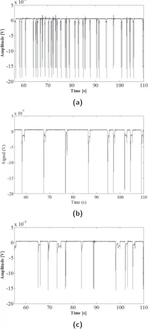
Based on the experimental setups used, two flow patterns can be clear distin-guished by visual inspection of the signal dynamics, defined as slow and fast. In the slow dynamics, the length of both air and water intervals can have significant variations during the experiment and the flow can be characterized by a sequence of smaller water intervals compared to the air intervals or vice versa (see Fig-ure 1.8(a) and (b)). In the fast dynamics, the length of air and water intervals are closer than in the previous case and during the time course, the significant changes cannot be detected in their lengths but in their distances. It can be inter-preted as a fast train of small air/water slugs of similar lengths (see Figure 1.8(c)

(25)

and (d)). The signals related to the slow patterns can be associated to a square wave trend and those related to the fast patterns to an oscillating behaviour. It can be verified that the transition point between the two dynamics is correlated to the input flow rates and the geometries. In case of experimental sets − 1/3 considering equal input flow rates, the fast dynamics were detected respectively at

f > 0.7 ml/min for {G1; G2} and at f > 3 ml/min for G3. It is worth to notice

that, the hydraulic resistances of G1 and G20 are greater than that of G30, so it was expected a transition for smaller flow rate in the experimental sets − 1/3 than in the set − 2. In case of experimental set − 2, due to the different values of two inputs flow rates, the fast dynamics were detected for {Vair; Vwater} both greater

than 1 ml/min.

Another important aspect is the possibility to trace out the information about the slugs length from the signals and the characteristics of the optical setup: the sam-ple frequency, the size of the optical window and objective magnification. During the fast patterns, in the experimental set − 2, a slug passage lasts on an average of 5 samples that is equivalent to 5 ms (based on optical setup − 1 where the sample frequency 1 kHz, the photodiode area 1 mm2 _{and objective magnification} 20X) whereas, in experimental set − 3, lasts on an average of 10 samples that is equivalent to 2.5 ms (based on optical setup − 2 where the sample frequency 4 kHz, the photodiode area 6 mm2 _{and objective magnification 10X).}

(26)

(a)

(b)

(c)

(d)

Fig. 1.8. Experimental set − 2. Signals related to one experiment per campaign: (a)

campaign−1 with AF = 0.158; (b) campaign−2 with AF = 0.794; (c) campaign−3

(27)

(a)

(b)

(c)

Fig. 1.9. Experimental set−3. Signals acquired with inputs flow rates f = 0.3 ml/min

in the selected channel positions. (a) A close to the inlet; (b)B at the channel length center; (c) C close to the outlet.

For the experimental set − 2, in campaigns − 1/2 for input flow rates ranges

f ≤ 1 ml/min, the slug patterns can be identified as slow dynamics. It is possible

to evidence in the signal trend that for campaign-1 the dominant input flow is the water (see Figure 1.8(a)) and air for campaign − 2 (see Figure 1.8(b)). Differently,

(28)

in campaign−3/4, for input flow rates f ≥ 1 ml/min, the fast dynamics are clearly distinguishable, and by visual inspection the dominant input flow cannot be de-tectable. In Figure 1.9 four experiments, one per campaign, were selected to sum up the signals features: Vwater = 0.64 ml/min, Vair= 0.12 ml/min (campaign −1,

AF = 0.158); Vwater = 0.16 ml/min, Vair = 0.60 ml/min (campaign − 2, AF =

0.794); Vwater = 6.4 ml/min, Vair = 1.2 ml/min (campaign − 3, AF = 0.158);

Vwater = 1.6 ml/min, Vair = 6.0 ml/min (campaign − 4, AF = 0.794).

For both the experimental sets − 1/3 only slow dynamics were considered, that allows to evince the signals changes also by visual inspection. In Figure 1.9, the signals acquired for input flow rate f = 0.3 ml/min in the three positions A, B, C are reported.

Four indicators were computed to classify flow patterns by the signals character-istics of the signal and to quantify the dynamics sensitivity to the experimental conditions. The indicator, named delta, was introduced for both slow and fast pat-terns, to quantify the air or water dominance in the micro-channel. Additionally, it was considered: for the slow patterns the slug passage in [ms] (named length), for the fast patterns the slugs inter-distance mean and variation (named spectrum peak and spectrum area).

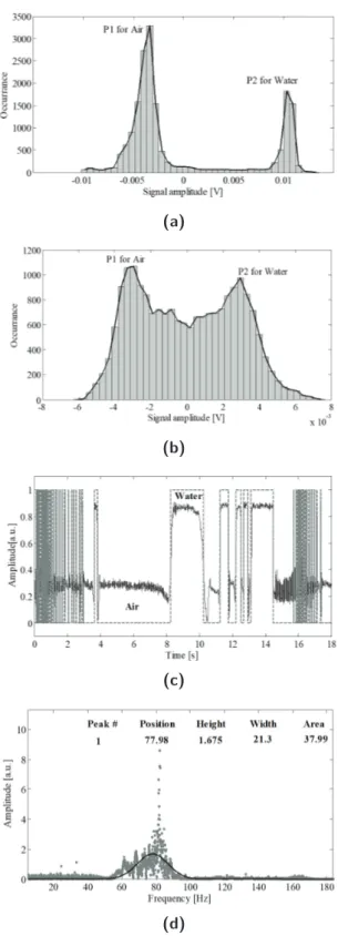
The delta was computed by statistical distribution of the acquired signals. It shows a bimodal shape in which the two peaks identify the presence of air (P1) and wa-ter (P2). Two examples of the bimodal distribution obtained for respectively slow and fast patterns are in Figure 1.10 (a) and (b). The delta was evaluated as the difference of two peaks amplitudes normalized in percentage, as in eq. 1.11. The positive values of delta are for the dominance of the water and negative for the air.

delta(%) = (P2− P1)

max(P1, P2) ∗ 100

(1.11) For the slow patterns, where it is possible to distinguish longer interval of water or air, the changes in the length of air and water intervals were considered. A square wave model was correlated to the signal trend (see Figure 1.10(c)) and a procedure based an adaptive threshold was used for its reconstruction. By means of this square model, it was possible to derive the length (in [ms]) of each water/air

(29)

interval and the number of intervals. Combining these two information the plot of trend of water/air intervals mean length in an experiment can be reconstructed as shown in Figure 1.11. It can be noticed that, the length trace could present some irregular peaks due to the unexpected longer air/water intervals compared with the value assumed on the average. In the results these outliers were neglected. For the fast patterns, by assuming constant the length for air and water slugs, as it can be drawn from the oscillating trend, the mean inter-distance and variability were computed. The content in the frequency domain, that is not significant in slow flow, becomes relevant, and the signal spectrum was used for the inter-distance evaluation. The spectrum profile was approximated with a Gaussian model to characterize the maximum in the spectrum and the area under the Gaussian curve (see Figure 1.10(d)) associated respectively to the mean slug interdistance and its variability. An iterative procedure, that uses an unconstrained nonlinear optimiza-tion algorithm to decompose the overlapping-peak signal into its components, was considered for the fitting in O’Haver [60]. By this Gaussian model it was possible to extract: the peak position in the spectrum, its amplitudes as well as the area under the Gaussian curve. The latter was considered proportional to the spectrum bandwidth. From a theoretical perspective, smaller is the bandwidth closer is the flow dynamics to a periodic behaviour, so this parameter can be used as indicator of the process nonlinearity.

(30)

(a)

(b)

(c)

(d)

Fig. 1.10. Slug patterns characterization by signal analysis. For the delta computation,

the bimodal distribution in case of (a) slow flows and (b) fast flows; (c) for the slow dynamics: fitting of the signal with a square wave model for the lengths of the air/ water intervals computation; (d) for the fast dynamics: fitting of the spectrum Gaussian profile and evaluation of the peak position, the amplitude, the area under the curve.

(31)

Fig. 1.11. Intervals length trace reconstruction by signal analysis for the experiment

(campaigns − 1/2, AF = 0.433): the water is in black line and air in dotted gray line.

1.5 Slug flows dynamics

1.5.1 _{Varying the micro-channel geometry (set − 1)}

Due to the experimental setting, for the input flow conditions f = {0.1, 0.3, 0.5}

ml/min the signals show a slow dynamics with long water intervals and smaller

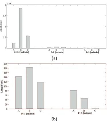
air slugs, as in experimental set − 3 (see Figure 1.9). The delta and the number of slugs intervals per minute per experiment were computed. In Figure 1.12(a) and Figure 1.13(a) the bar diagrams related to the delta values and the number of intervals at the different the input flow rate conditions are represented for both geometries {G1; G2}. In Figure 1.12(b) and Figure 1.13(b) the trends of these parameters obtained by the values interpolation versus the input flow conditions

f = {0.1, 0.3, 0.5} ml/min per {G1; G2} are represented. In the Figure 1.12(b)

and Figure 1.13(b), respectively, the delta decreases and the number of intervals increases following a linear trend in case of the straight channel and a parabolic trend in the serpentine. Being the hydraulic resistance of the straight channel (Rh1) three time greater than the one of the serpentine (Rh2) a faster change in both these parameters was expected. Nevertheless, it is possible to notice that dis-tances between the parameters trends for G1 and G2 are not conservative respect to the ratio of 3 increasing nonlinearly with the input flow rates. That confirms the higher sensitivity to the input flow conditions in the straight channel compared with the curved one, so the robustness introduced into the processes by a winding geometry.

(32)

(a) (b)

Fig. 1.12. Experimental set − 1. (a) Delta bar diagram and (b) the trends obtained

by values interpolation versus the input flow conditions f = {0.1, 0.3, 0.5} ml/min per {G1; G2}.

(a) (b)

Fig. 1.13. Experimental set − 2. (a) Number of intervals per minute bar diagram

and (b) the trends obtained by values interpolation versus the input flow conditions

f = {0.1, 0.3, 0.5} ml/min per {G1; G2}.

1.5.2 _{Varying the input flow rate (set − 2)}

In campaigns − 1/2 for input flow rates f ≤ 1 ml/min the signals show slow dynamics and no bands of interest are detected in the spectra. Differently in

campaigns−3/4 for input flow rates f ≥ 1 ml/min the signals show fast dynamics

and it is always possible to identify in the spectra a band of interest.

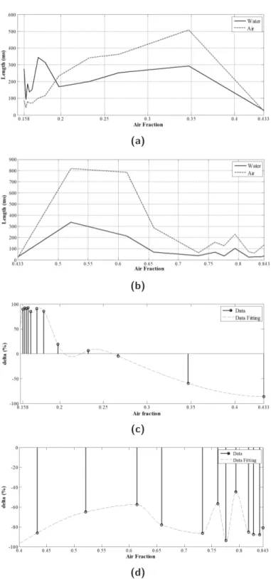
In Figure 1.14 the results obtained per experiment in the campaigns − 1/2 are summarized. Figure 1.14(a) and (b) report the average length in [ms] of the air (gray line) and water (black line) slugs versus the AF respectively in campaign −1 and campaign−2. In campaign−1, the air slugs are longer than those of water for

(33)

AF > 0.19, while in campaign − 2 in all the AF range. At the value AF ∼= 0.43, present in both campaigns, the length of the air and water intervals are equal. For 0.19 < AF < 0.40 and 0.46 < AF < 0.70 respectively in campaign − 1 (see Figure 1.14(a)) and campaign − 2 (see Figure 1.14(b)) air and water intervals increase and decrease with a parabolic trend can be identified.

In campaign − 1, the air intervals are in the range [50 − 500] ms and the water intervals in the range [50 − 350] ms, both the mean length of the air and water intervals increase until AF = 0.35. In campaign − 2 the air intervals are in the range [50 − 800] ms and the water intervals in the range [50 − 350] ms, both the mean length of the air and water intervals increase until AF = 0.521. In

campaign − 1 for AF < 0.19 a second smaller parabolic trend was detected in

which the water interval are bigger than the water, but no correlation between the two trends is visible. Finally, in campaign for the AF > 0.73 a stable behaviour arises in which both intervals are almost unvaried: the mean length of the water slugs is around 50 ms and of the air slugs 150 ms.

In Figure 1.14(c) and (d) the bar diagrams related to the delta values versus the AF respectively in campaign − 1 and campaign − 2 are plotted. In campaign − 1, consistently with the previous results, a stronger water dominance up the 90% can be found for AF < 0.19, and then a slow decrease leads to the air dominance for

AF > 0.23. This trend lasts until the AF = 0.43 with a delta around −95%. In campaign − 2 the delta is always negative, meaning air dominance. For 0.43 < AF < 0.733 the subsequent delta increase and decrease reflects the sensitivity to

the air and water slug length increase and decrease. The oscillating value for the 0.733 < AF < 0.817 in the range [−95%; −50%] can be correlated to a transitory behaviour before the stabilization. It is worth to notice that in both campaigns the trends of the air and water mean length are mainly specular respect to the AF value 0.433, irrespectively of which input flow rate is dominant.

(34)

(a)

(b)

(c)

(d)

Fig. 1.14. Experimental set − 2 with f < 1 ml/min. The intervals average length of

the air (dotted line) and water (black line) slug versus AF in the campaign − 1 (a) and in the campaign − 2 (b); The delta value versus AF in the campaign − 1 (c) and in the campaign − 2 (d).

(35)

The maximum mean length of the air in campaign − 2 is 800 ms greater than the one in campaign − 1 (300 ms), while the maximum mean of the water length is around 300 ms in both cases. It is important to underline that, considering an experiment with longer slugs, to have a significant number of slugs a longer time interval is necessary.

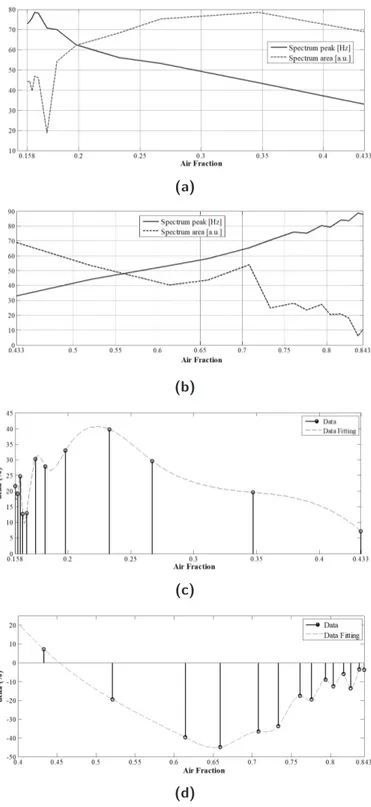
In campaigns − 3/4, for the experimental campaigns with f > 1 ml/min, the Figure 1.15(a) and (b) report the position of the peak in the spectrum (black solid line) and the value of area under the Gaussian (gray dotted line) versus AF, respectively, for campaigns − 3/4. The frequency peak trend decreases almost linearly in campaing − 3 in [30, 90] Hz and then increases in the same range in campaign − 4. An opposite behaviour is shown for the Gaussian area: its lowest values is around 30 [a.u.] in campaign − 3 and 10 [a.u.] in campaign − 4. This translation of the peak position in the spectrum reflects the changes in the interdistance between slugs. The higher frequencies, so the smaller inter-distances, were for low value of AF in campaign − 1 and high in campaign − 2. For the same AF values the area under the Gaussian curve decreases leading to a reduction in the inter-distance variability. It means that, increasing the input flow rate it is possible to obtain dynamics in which the nonlinearity effects are reduced, toward a tendency to an oscillating periodic behaviour. In Figure 1.15(c) and (d), the bar diagrams related to the delta variation versus AF respectively for

campaign − 3 and campaign − 4 are shown. In campaign−3 there is always water

dominance, while in the campaign−4 the delta (Figure 1.15(d)) initially is positive (water dominance) then for AF = 0.521 becomes negative (air dominance). For

AF ≤ 0.167 in campaign − 3, for AF > 0.817 in campaign − 4 the delta values are

smaller and oscillating respectively around 20% and −5%. The reduction of delta was obtained because the two peaks have close amplitude, and it is correlated with the same length of the air and water intervals. ForAF = 0.233 in campaign − 3 and AF = 0.614 in campaign − 4 the maximum delta values are obtained around ±40%. Both results confirm that the increase of input flow rate produces a effect on the slug displacement along the micro-channel leading to a stabilization of the process toward a periodic regime where the length of the air and water interval are closer.

(36)

(a)

(b)

(c)

(d)

Fig. 1.15. Experimental set − 2 with f > 1 ml/min. The position of the peak in the

spectrum (black line) and the area under the Gaussian (dotted line) versus AF in the

campaign − 3 (a) and in the campaign − 4 (b); The delta value versus AF in in the campaign − 3 (c) and in the campaign − 4 (d).

(37)

1.5.3 _{Varying the investigation points (set − 3)}

Due to the experimental setting, for all the input flow conditions f = {0.3, 1, 3}

ml/min the signals show slow dynamics with long water intervals and small air

slugs, this was important for the characterization of the behaviour at the different positions {A, B, C} of the micro-channel.

In Figure 1.16, the bar diagrams related to the delta value for the three flow rates and the three selected positions are shown. It is possible to notice that there is water dominance with a positive delta value in a range of [80%; 90%]. The delta at the points (A, B) is similar, while it changes at the point C, becoming slightly greater for f = 0.3 ml/min and smaller for f = {1, 3} ml/min. The growth of delta in point C for f = 0.3 ml/min could due to a predominant effect of the curves inducing a slowdown of the process at the outlet. From the other hand, the delta reduction in point C for f = {1, 3} ml/min can be related to output pressure increase for higher slug velocity. As a consequence of the air compression in the position C, the air slugs mean lengths are always less than in the other positions, this effect is amplified by the flow velocity. In Figure 1.17 and Figure 1.18 the mean length in [ms] of respectively the air and water intervals are reported for the three positions. The Figure 1.17(a) and Figure 1.18(a) show the results for the three input flow rates f = {0.3, 1, 3} ml/min, while the Figure 1.17(b) and Figure 1.18(b) report a zoom on for f = {1, 3} ml/min.

That was necessary because the mean length for f = 0.3 ml/min is definitely greater than in the other two flow conditions, for example in point B for f =

Fig. 1.16. Experimental set − 3. Delta value for f = {0.3, 1, 3} ml/min in the section

(38)

(a)

(b)

Fig. 1.17. Experimental set − 3. The average length of the air intervals in the channel

positions {A, B, C} respectively close to the inlet, at the center and close to the outlet; (a) f = {0.3, 1, 3} ml/min; (b) a zoom for f = {1, 3} ml/min.

{0.3, 1, 3} ml/min the water slug length is respectively {3.5; 0.6; 0.1} s for the air and {20; 0.18; 0.06} s for the water. It is possible to notice that both the mean air and the water intervals lengths are sensitive at the same way to the acquisition points and the input flow rates.

In addition, it is possible to detect how the dynamics at the inlet is affect by the increasing of the flow. In both the experiments with the f = {0.3; 1} ml/min a Gaussian profile is detectable, so the mean slug length increases at the center of the channel (B) and decrease at the inlet and outlet.

Coherently with the analysis by delta, the mean of the slug length is lower in po-sition C compared to popo-sition A for f = {1; 3} ml/min, while for f = 0.3 ml/min the process slows down for the curved geometry inducing at an increase of the bubble length at the outlet.

(39)

(a)

(b)

Fig. 1.18. Experimental set − 3. The average length of the water intervals in the

channel positions {A, B, C} respectively close to the inlet, at the center and close to the outlet; (a) f = {0.3, 1, 3} ml/min; (b) a zoom forf = {1, 3} ml/min.

the mean slug length is greater at the center than at the inlet, compared with

f = 3 ml/min in which the situation is opposite. The profile across three

acquisi-tion posiacquisi-tions is decreasing, so the slug length decreases along the channel due to the input flow pressure increase.

A systematic experimental study on the slug flow patterns generation in an hori-zontal curved micro-channels of {320; 640} µm width, where a continuous slug flow was generated by two upstream of water and air, is presented. The attention has been focused on three issues: the difference in the slug displacement in a straight channel compared with a serpentine; the role played by the input flow rates in the slugs flow patterns classification and the flow changes in different channel posi-tions.

The photodiode signals acquired in all the experiments were analyzed, and orga-nized in three experimental sets based on the investigated aspects. A classification

(40)

of the obtained slugs dynamic in slow and fast flow patterns was established, in slow patterns the long air intervals are combined with short water intervals (or vice versa), while in fast patterns both intervals are small and similar. The depen-dence of transition point between the two slugs regimes on the channel geometry and input flow rate was evinced.

From the experimental set − 1 it was highlighted the difference in the flows gen-erated in the straight and serpentine micro-channels but, above all, that by the serpentine geometry the robustness of the microfluidic processes to the flow input variations can be improved and controlled easily, also in fast conditions. From the experimental set − 2, the changes in the flow due to the input flow rates for both slow and fast patterns in a serpentine was analyzed by the introduction of four indicators: the delta for the air/water presence, the slug length for slow patterns and the slug interdistance for fast patterns. In the slow flows, for f < 1 ml/min, it was possible to notice that the air plays always a fundamental role and becomes dominant for AF > 0.2. Varying the AF, a synchronous increase and decrease of both air and water slugs lengths on different levels occurs and, only for AF > 0.7, their values are almost unvaried and stable: the air bubble lengths are almost three time greater than the water length. Based on that it is possible, in a generic geometry, to establish which flow rate gives a specified slug behaviour, although to quantify the exact value of the length is necessary to take into account the channel hydraulic resistance. In the fast flow for f > 1 ml/min, increasing both air or water, the mean slug inter-distance and its variability is reduced, leading to a process stabilization toward a periodic regime. A fast train of small slugs can be produced with a modulation of the velocity set by the input flow rate with an a priori known uncertainty.

From the results of experimental set − 3, it was possible to conclude that for slow input flow rates, the slowdown of the process induced by the curves is predomi-nant and leads to an increase of the slug length at the outlet, while for fast input flow rates the increase of air compression, induced by the flow velocity, brings a reduction of the slug length along all the channel.

The results obtained highlight the advantages in the process control introduced by curve geometry, despite the presence of nonlinear phenomena. Technologically, the processes classification obtained by a simple analysis of optical signals, instead of

(41)

using costly and bulky equipment or invasive process detection systems represents a proof of concept for a future integration of both the detection and flow control in a single micro-system.

(42)

Chapter 2 Slug flows modelling by nonlinear

systems synchronization

2.1 Experimental campaigns

The setup considered is the same described in Chapter 1, labelled setup − 1. The serpentine micro-channel G3 (w = 640 µm, l = 121 mm) was used (see Figure 1.4). The process was monitored at the center of straight part, tagged as point B in the figure. The signals acquired from the photodiodes were filtered, as described in detail in paragraph 1.2.

Two sets of 9 experiments were performed, where Vair and Vwater represent the

volumetric flow rates. To have a fast flow the input flow rates were set always greater than 1 ml/min.

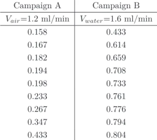
In campaign−A, the air flow was fixed to Vair = 1.2 ml/min and in campaign−B

the water flow rate was Vwater = 1.6 ml/min. The second input flow rate was

varied leading to different AF values per experiment (computed as in eq. 1.10) reported in Table 2.1. In campaign − A the water dominance leads the AF in the range [0.158 − 0.433] and in campaign − B the air dominance brings the AF to [0.433 − 0.804].

The values of the input flow rate were set considering the Capillary number and the Reynolds number. The Ca was always of the order of 10−3_{, that confirms} the theoretical expectancy of the slug formation. The Re was in the range Re ∈

(43)

Slug flows modelling by nonlinear systems synchronization 36

[9.26 − 26.71] at the boundary with the laminar flow condition (Re > 10).

Tab. 2.1. The Air Fraction (AF ) values per experiment in the Campaigns A and B. Campaign A Campaign B

Vair=1.2 ml/min Vwater=1.6 ml/min

0.158 0.433 0.167 0.614 0.182 0.659 0.194 0.708 0.198 0.733 0.233 0.761 0.267 0.776 0.347 0.794 0.433 0.804

2.2 Slug flows nonlinear characterization

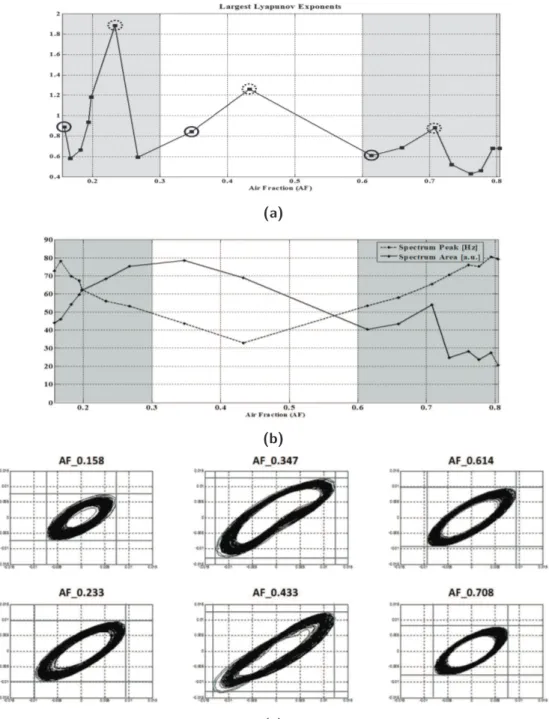
In [48], it has been widely investigated the nonlinearity of the slugs flow and its classification through nonlinear indicators. Nonlinear time series analysis [61] has been applied to the experimental data in order to quantify the flow patterns and the bubbles’ dynamics in terms of Largest Lyapunov exponent (LE). In Figure 2.1(a), considering both experimental campaigns, the values of LEs versus the AF are plotted. The two shaded areas are for the water dominance with AF ∈ [0.1, 0.3] and air dominance with AF ∈ [0.6, 0.8]. In the range AF ∈ [0.3, 0.6], the amount of air and water fed in the channel are almost balanced. A local peak associated with a rise in the LE trend and subsequently a drop can be detected in all the three areas.

For a in-depth analysis of the data, the frequency analysis of the time series was performed.

The obtained broadband spectrum resembles a bell-shaped curve, then its pro-file was approximated with a Gaussian model to characterize the peak in the spectrum and the area under the Gaussian curve, associated respectively to the mean slug inter-distance and its variability. The area under the Gaussian curve was considered proportional to the spectrum bandwidth. From a theoretical

(44)

per-Slug flows modelling by nonlinear systems synchronization 37

(a)

(b)

(c)

Fig. 2.1. (a) Largest Lyapunov exponent values versus the AF; the circled points are

related to the conditions selected for the attractors reconstruction; (b) The frequency peak (gray dotted line) and area under the Gaussian (black solid line) versus the AF; (c) State-space representations at the top the experiments with AF = [0.158, 0.347, 0.614], while at the bottom the experiments with AF = [0.233, 0.433, 0.708].

(45)

spective, smaller is the bandwidth closer is the flow dynamics to a periodic be-havior. The Figure 2.1(b) shows the peak frequency (grey dotted line) and the value of the area under the Gaussian (black solid line) versus AF. Corresponding to the water and air dominance, respectively, in the ranges AF ∈ [0.1, 0.2] and

AF ∈ [0.7, 0.8], both trends show that the mean bubble inter-distance increases

and its variability decreases. It can be confirmed by the two saddle points in the LE trend (Figure 2.1(a)) and proves that the process nonlinearity can be reduced by the increase in one input flow rate.

In Figure 2.1(c), the attractors obtained by the state space reconstruction in the six experiments, circled in Figure 2.1(a), are shown to give a visual characteriza-tion of the flow nonlinearity. At the top, there are the three experiments with the lowest LE values for AF = [0.158, 0.347, 0.614] and, at the bottom, the experi-ments with the highest LE values for AF = [0.233, 0.433, 0.708]. The attractors comparison remarks that the stretching is greater when in the micro-channel there is no air or water dominance and the two phases are balanced. It is important to evidence that the attractors shape is always a single scroll.

2.3 Master-Slave synchronization

One property of the chaotic systems is the sensitivity to initial conditions, thus two identical systems starting from slightly different points in the state space evolve, in long-term, in a totally uncorrelated manner. The synchronization ap-proach allows to drive the two systems toward a correlated time evolution. The two systems are named as Master and Slave. In this contest, the synchronization theory was used as a framework for the modelling and identification of real-world processes by means of experimental data.

The synchronization schemes are classified in two main classes: unidirectional or bidirectional coupling. In the identification process it is useful to use an unidi-rectional synchronization scheme that considers only how one system (Master) can affect a second system (Slave). Particularly, in the method of decomposition

into sub-systems, the Slave system can be decomposed at least into two

(46)

the drive system to follow a definite state variable (driven variable). It has been demonstrated that with this procedure the systems synchronize also in presence of noise [62]. Following this scheme and assuming a time series as a state variable of an unknown Master system, it can be estimated an optimal set of parameters of a Slave known model to reach the synchronization between the asymptotic time evolution of at least one of its state variables and the experimental data used to drive it [63].

It is possible to distinguish four main classes of synchronized behavior [64]: com-plete synchronization (CS) consists in a perfect matching of the two chaotic trajec-tories, the systems forget their initial conditions continuing to evolve chaotically; phase synchronization (PS) occurs in oscillators when their phases are locked, while amplitudes remain almost uncorrelated; lag synchronization (LS) occurs when the two trajectories are locked both in phase and amplitude but with a finite time lag; generalized synchronization (GS) is achieved when the dynamics of one of the coupled systems can be expressed as a function of the other dynamics.

The phase or lag synchronization are most significative being the slug passage in the flow strictly related to the frequency and the phase of the signal more than to its amplitude.

The experimental time series acquired from the microfluidic process, Ym, was

as-sumed as the asymptotic behavior of a generic state variable of an unknown Master system and this information was used to drive a Slave system with a known model with undefined parameters. The Slave system selected was the Chua’s oscilltaor model being a nonlinear systems capable of reproducing a great number of experi-mental phenomena [46]. The dimensionless state equation of the Chua’s oscillator follows. dx dt = kα(y(t) − x(t) − f(x(t))) (2.1) dy dt = k(x(t) − y(t) + z(t)) (2.2) dz dt = k(−βy(t) − γz(t)) (2.3)

(47)

f (x(t)) = m1x(t) + 1

2(m0 − m1) {| x(t) + 1 | − | x(t) − 1 |} (2.4) where x, y, and z are the state variables and α, β, γ, m0 and m1 the parameters. The unidirectional synchronization scheme based on the decomposition method was used and the Master-Slave system equations were re-written as follows:

dx(t)

dt = kα(Ym(t) − x(t) − f(x(t))) (2.5)

dz(t)

dt = k(−βYm(t) − γz(t)) (2.6)

where the microfluidic time series Ym affects the sub-system formed by the x and z

variables of Chua’s model. The drive sub-system of eqs.2.5-2.6 is solved by using the Dormand-Prince method [65] with fixed time-step Ts.

The equation related to the variable y is decoupled from the system and used to verify the convergence criteria, as in the following equations:

dy

dt = k(x(t) − Ym(t) + z(t)) (2.7)

limt→∞| y(t) − Ym(t) |= 0 (2.8)

The eq. 2.8 was implemented using as optimization method the genetic algorithm (GA) [47]. The optimal value of the parameters set {α, β, γ, Ts} that minimizes

the error fitness function was searched in eq. 2.9. The parameter Ts is the sample

step used during the simulation and it was included in the parameter set to be tuned with the changes in the time series due to the sample frequency at different slug flow velocities.

The root mean square error between the time series Ym and the y state variable

of the Chua’s oscillator was chosen as error index (see eq. 2.9).

I{α, β, γ, Ts} =

ó qN

n=1(Ym(n) − y(nTs))2

N (2.9)

By a visual inspection of the Chua single-scroll attractor that can be obtained by tuning the parameters of the model [46], it was selected the one reported in plate

Models and Systems for the Control of Two-Phase Processes in Microfluidics

Fabiana Cairone

Models and Systems for the

control of two-phase processes

in microfluidics

Doctor of Philosophy in Ingegneria dei Sistemi, Energetica,

Informatica e delle Telecomunicazioni

UNIVERSITÀ DEGLI STUDI DI CATANIA

Doctor of Philosophy in Ingegneria dei Sistemi,

Energetica, Informatica e delle Telecomunicazioni

Models and Systems for the control

of two-phase processes in

microfluidics

Contents

I

SLUG FLOWS IN MICROFLUIDICS

1

II

MICRO-OPTOFLUIDICS DEVICE FOR SLUG FLOWS

DETECTION

86

Abstract

Introduction

Part I

SLUG FLOWS IN

MICROFLUIDICS

Introduction

Chapter 1

Slug flows in micro-channels

1.1

Theoretical background

1.2

Experimental setup

1.3

Experimental campaigns

1.4

Indicators for slug flows characterization

1.5

Slug flows dynamics

1.5.1

Varying the micro-channel geometry (set − 1)

1.5.2

Varying the input flow rate (set − 2)

1.5.3

Varying the investigation points (set − 3)

Chapter 2

Slug flows modelling by nonlinear

systems synchronization

2.1

Experimental campaigns

2.2

Slug flows nonlinear characterization

2.3

Master-Slave synchronization

_{Varying the micro-channel geometry (set − 1)}

_{Varying the input flow rate (set − 2)}

_{Varying the investigation points (set − 3)}