UNIVERSITY OF CALABRIA
Department of Computer Engineering, Modelling, Electronics and Systems Science
Ph.D. Thesis in
Information and Communication Technologies
Global Optimization, Ordinary Differential Equations
and Infinity Computing
Marat S. Mukhametzhanov
Scientific Advisor
Coordinator
Prof. Yaroslav D. Sergeyev
Prof. Felice Crupi
Contents
Introduction 7
1 Univariate Lipschitz Global Optimization 15
1.1 Acceleration techniques in Lipschitz global optimization . . . . 16 1.1.1 Local Tuning and Local Improvement techniques . . . 17 1.1.2 Convergence study and experimental analysis . . . 27 1.2 Solving practical engineering problems . . . 37
1.2.1 Applications in noisy data fitting and electrical
engineering . . . 38 1.2.2 Experimental study . . . 40 2 A Systematic Comparison of Global Optimization Algorithms
of Different Nature 53
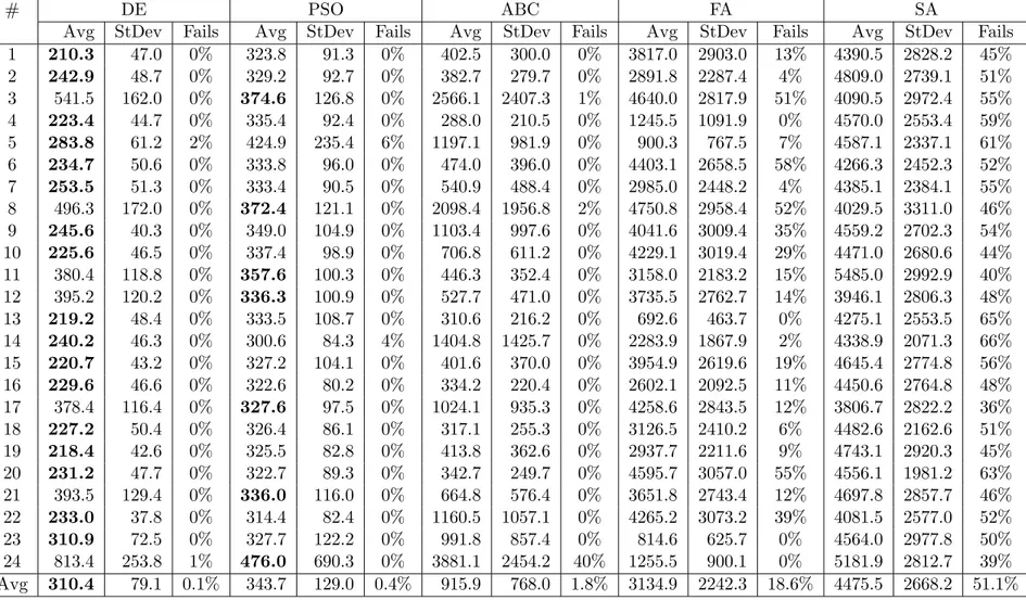
2.1 Numerical Comparison of Nature-Inspired Metaheuristics Using Benchmarks . . . 54 2.1.1 Description of algorithms . . . 55 2.1.2 Results of the comparison . . . 57 2.2 A systematic comparison using classes of randomly generated
test problems . . . 71 2.2.1 Operational zones for comparing metaheuristic
and deterministic univariate algorithms . . . 71 2.2.2 Techniques for comparing multidimensional stochastic
and deterministic methods . . . 80 2.2.3 Aggregated operational zones and restarts of
metaheuristics . . . 85 2.3 Emmental-type GKLS-based generator of test classes for
glo-bal optimization with nonlinear constraints . . . 98 2.3.1 Box-constrained GKLS generator of test problems . . . 99 2.3.2 Generator with parameterizable difficulty and
6 Contents 3 Handling of Ill-Conditioning in Optimization via Infinity
Computing 113
3.1 Infinity Computing methodology . . . 114 3.2 Strong homogeneity of a class of global optimization
algorithms working with infinite and infinitesimal scales . . . . 121 3.2.1 A class of global optimization problems with infinite
and infinitesimal Lipschitz constants . . . 122 3.2.2 Univariate Lipschitz global optimization algorithms and
strong homogeneity . . . 127 3.3 Numerical infinitesimals in convex non-smooth
optimization . . . 137 3.3.1 Variable metric method based on the limited-memory
bundle approach . . . 138 3.3.2 Handling of ill-conditioning using infinitesimal
thresholds and Grossone-D-Bundle method . . . 141
4 Infinity Computing and Ordinary Differential Equations 153
4.1 Generalized Taylor-based methods in standard and infinity floating-point arithmetic . . . 154 4.2 Convergence and stability analysis of the proposed one-step
multi-point methods . . . 165 4.3 Taylor-Obrechkoff method of order 4 using exact derivatives . 179
Conclusion 187
Acknowledgements 193
Bibliography 195
Introduction
The main research topic studied in this work is global optimization—a field studying theory, methods, and implementation of models and strategies for solving multiextremal optimization problems. The rapidly growing interest to this area is explained by both the raising number of applied decision-making problems, that are described by multiextremal objective functions, and the significant recent development of advanced computer facilities.
Global optimization problems arise frequently in many real-life applicati-ons [88, 152, 157, 192, 215, 229]: in engineering, statistics, decision making, optimal control, machine learning, etc. A general global optimization pro-blem requires to find a point x∗ and the corresponding value f (x∗) being the
global (i.e., the deepest) minimum of a function f (x) over an N−dimensional domain D, where f (x) can be non-differentiable, multiextremal, hard to eva-luate even in one point, and given as a “black box”. Therefore, traditional local optimization methods [141, 145] cannot be used in this situation.
One of the important applied fields of efficient global optimization met-hods is the investigation of control systems under uncertain values of their parameters, in order to afford the desired safe functioning of a controlla-ble object. For example, many important procontrolla-blems of robust control can be reduced to the problem of establishing the positiveness of multiextremal functions. This problem can be successfully solved with the availability of global optimization methods: it is sufficient to establish that the global mi-nimum of a function describing the system is positive.
It can be noted in this context that not only multidimensional global optimization problems but also univariate problems of this kind arise fre-quently in different real-life applications, for instance, in engineering (see, e. g., [82, 93, 105, 113, 230]) and statistics (see, e. g., [26, 68, 72]). In par-ticular, in structured low rank approximation (see, e. g., [74]), it can be necessary to solve perturbed problems as well as the original ones. The Lip-schitz constant for the objective function in that case can be very large and the problem becomes very difficult to solve. Electrical engineering applica-tions (see, e. g., [28, 38, 113, 190, 191, 183, 215]) can also require Lipschitz
8 Introduction global optimization, for example, for solving the minimal root problem (see, e. g., [114, 193, 189]). This kind of problems very often can be met in the multidimensional case, as well (see, e. g., [13, 120, 149, 151, 207]).
In the global optimization literature, there exist several ways to consider various global optimizations strategies (see, e. g., [144, 152, 154]). Such con-siderations are usually either ‘problem-oriented’ or ‘methodology-oriented’. The problem-oriented point of view takes into account the problem infor-mation which can be used by a method during the search for the global solution. For example, in continuous global optimization, derivative-free or derivative-based methods can be considered depending on whether the ob-jective function and constraints are differentiable and the derivatives can or cannot be computed or estimated.
The methodology-oriented point of view is more suitable for black-box problems and mainly based on the methodology applied for solving these problems. For example, global optimization algorithms can be divided into deterministic and stochastic. Assuming exact computations and arbitra-rily long run time, deterministic methods ensure that after a finite time an approximation of a global minimizer will be found (within prescribed tole-rances). Stochastic methods only offer a probabilistic guarantee of locating the global solution: their convergence theory usually states that the global minimum will be identified in an infinite time with probability one.
Among the vast group of deterministic algorithms for solving black-box global optimization problems the so-called direct (or derivative-free) search methods should be mentioned (see, e.g., [30, 33, 122, 158]). They are fquently used in engineering design (as, e.g., the DIRECT method, the re-sponse surface, or surrogate model methods, pattern search methods, etc.; see [54] for details). Black-box global optimization techniques based on an adaptive sampling and partition of the domain D are also widely used in practice (see, e.g., [89, 151, 152, 189, 216]).
Adaptive stochastic search strategies are mainly based on random sam-pling in the feasible set. Such techniques as adaptive random search, simu-lated annealing, evolution and genetic algorithms, tabu search, etc., can be cited here (see [54, 134, 147, 157, 224] for details). Stochastic approaches can often deal with the described black-box problems in a simpler manner than the deterministic algorithms (being also suitable for the problems where the evaluations of the functions are corrupted by noise). However, there can be difficulties with some of these methods, as well (e.g., in studying con-vergence properties of metaheuristics). Several restarts can also be involved, requiring more expensive functions evaluations. Moreover, solutions found by many stochastic algorithms (especially, by popular heuristic nature-inspired methods like evolutionary algorithms, simulated annealing, etc.; see, e.g.,
9 [97, 98, 147, 161, 224]) can be only local solutions to the problems, far from the global ones. This can preclude such methods from their usage in practice, when an accurate estimate of the global solution is required.
Obviously, the problem of a comparison of existing numerical algorithms for solving global optimization problems arises. The traditional way to do this is to use a collection of test functions and to show that on this collection a new method is better in some sense than its competitors. Then, a trade-off between the number of test functions, reliability of the comparison, and visibility of results arises. Clearly, a small number of test functions does not lead to a reliable comparison and a huge number of functions produces huge tables with a lot of data that sometimes are difficult for a fast visualization and an immediate comprehension.
Another difficulty in a convincing demonstration consists in the existence of methods having a completely different structure. A typical example is the principle trouble arising when one needs to test a deterministic method A with a stochastic algorithm B. The method A applied to a certain set of functions returns always the same results while the method B should be run several times and the results of these runs are always different. Consequently the method A is compared with some average characteristics of the method B. In the literature, there exist some approaches for a graphical comparison of methods, as for example, operational characteristics (proposed in 1978 in [78], see also [214, 215]), subsequently generalized as performance profiles (see, e. g., [46]) and re-considered later as data profiles (see, e. g., [141]). Alt-hough they are very similar, performance profiles are mainly based on the relative behavior of the considered solvers on a chosen test set, while opera-tional characteristics (and data profiles, which are quite close to operaopera-tional characteristics) are more suitable for analyzing performance of a black-box optimization solver (or solvers) with respect to expensive function evaluati-ons budget, independently of the behavior of the other involved methods on the same benchmark set.
All these techniques are, however, not always suitable for the comparison of methods of a different nature (for example, metaheuristics having a sto-chastic nature and deterministic Lipschitz methods), although an attempt of the usage of operational characteristics to study the behavior of a method with different parameters’ values has been made in [214].
Today, a rapidly growing interest to modern supercomputers leads to the necessity of development of new algorithms and methods for working with novel supercomputing technologies (e.g., [169] for Infinity Computing, [19] for Quantum Computing, [2] for Biocomputing, etc.). In this work, the Infinity Computing, a novel methodology allowing one to work numerically with infinite and infinitesimal numbers, is studied.
10 Introduction This numeral system proposed in [172, 176, 180] is based on an infinite unit of measure expressed by the numeral ① called grossone and introduced as the number of elements of the set N of natural numbers (a clear difference with non-standard analysis can be seen immediately since non-standard in-finite numbers are not connected to concrete inin-finite sets and have a purely symbolic character). Other symbols dealing with infinities and infinitesimals (∞, Cantor’s ω, ℵ0, ℵ1, ..., etc.) are not used together with ①. Similarly,
when the positional numeral system and the numeral 0 expressing zero had been introduced, symbols V, X, and other symbols from the Roman numeral system had not been involved.
In order to see the place of the new approach in the historical panorama of ideas dealing with infinite and infinitesimal, see [100, 125, 126, 128, 138, 174, 175, 185]. In particular, connections of the new approach with bijections are studied in [128] and metamathematical investigations on the theory and its non-contradictory can be found in [126]. The new methodology has been successfully used in several fields. We can mention numerical differentiation and optimization (see [39, 177, 233]), models for percolation and biologi-cal processes (see [91, 92, 179, 219]), hyperbolic geometry (see [129, 130]), fractals (see [91, 92, 171, 173, 179]), infinite series (see [96, 174, 178, 228]), lexicographic ordering, and Turing machines (see [175, 185, 186]), cellular automata (see [34, 35, 36]), etc.
It is well-known that in ill-conditioned systems, numerical methods can lead to incorrect results. However, it has been shown in [180], that in some cases ill-conditioning can be avoided using ① and the well-known Gauss met-hod can be used without pivoting to solve the systems of linear equations. So, it can be very advantageous to use Infinity Computing to handle with ill-conditioning in optimization, as well. In this work, the advantages of ap-plying the Infinity Computing are studied with respect to the traditional methodologies in order to handle with ill-conditioning occurred in optimiza-tion.
It should be noticed that the advantages of the Infinity Computing are not limited to working with ill-conditioning only. It has been shown in [181], that the numerical derivatives of a black-box function y(x) can be calculated exactly using ①. Moreover, it has been also shown that the derivatives can be calculated exactly even if the function y(x) is not given explicitly, but it is a solution to some ordinary differential equation. So, in this work, the advantages of the Infinity Computing are studied in the field of ordinary differential equations, as well.
The main aims of this research can be formulated as follows.
11 univariate Lipschitz global optimization and new algorithms based on them.
– Theoretical and experimental study of the proposed algorithms.
– Development of new efficient methodologies allowing one to compare graphically global optimization algorithms of a different nature. – Massive experimental comparison of several widely-used nature-inspired
metaheuristic algorithms with several deterministic approaches using the proposed comparison techniques.
– Development of a new generator of multidimensional test problems with non-linear constraints, based on the GKLS generator of box-constraints test problems, allowing one to test different constrained global optimi-zation algorithms.
– Application of the Infinity Computing in order to handle with ill-conditi-oning occurred in optimization. In particular, two different applications are considered: univariate Lipschitz global optimization problems and multidimensional convex non-smooth optimization problems.
– Development of new explicit and implicit methods for solving ordinary differential equations on the Infinity Computer and a theoretical study of their convergence properties.
Scientific novelty and practical importance of the present research consists of the following:
– Several new ideas that can be used to speed up the search in the framework of univariate Lipschitz global optimization algorithms are introduced. Proposed local tuning and local improvement techniques can lead to significant acceleration of the search and enjoy the following advanta-ges:
– the accelerated global optimization methods automatically realize a local behavior in the promising subregions without the necessity to stop the global optimization procedure;
– all the evaluations of the objective function executed during the local phases are used also in the course of the global ones.
It should be emphasized that proposed global optimization methods have a similar structure and a smart mixture of new and traditio-nal computatiotraditio-nal steps leads to 22 different global optimization al-gorithms. All of them are studied and compared on several sets of
12 Introduction tests. Performed numerical experiments confirm the advantages of the proposed techniques.
– Two practical engineering problems are studied: finding the minimal root of a non-linear equation problem from electrical engineering and a sum of damped sinusoids from noisy data fitting. Numerical experiments on the presented classes of engineering problems confirmed the advantages of the proposed techniques, as well.
– Two efficient methodologies allowing one to compare global optimization algorithms of different nature, called “Operational zones” and “Aggre-gated operational zones”, are proposed in this work. A massive ex-perimental study of several widely-used nature-inspired metaheuristic and deterministic global optimization algorithms is performed on more than 1000 test problems with more than 1 000 000 runs. It is shown that this new graphical methodology for comparing global optimiza-tion methods of a different nature is quite representative. Almost all qualitative characteristics that can be studied from numerical tables can be also observed from operational zones. Moreover, the best, the worst, and average performances of stochastic methods can be easily found, as well.
– Collections of test problems are used usually in the framework of continu-ous constrained global optimization (see, e.g., [53]) due to absence of test classes and generators for such a type of problems. This work in-troduces a new generator of test problems with non-linear constraints, known global minimizers, and parameterizable difficulty, where both the objective function and constraints are continuously differentiable. – Application of the Infinity Computing in order to handle of ill-conditioning
in optimization shows promising results. In particular, we show in this work that several ill-conditioned problems in the traditional compu-tational framework become well-conditioned if the Infinity Computing is applied. Presented techniques can be used in different fields, where ill-conditioning appears.
– Finally, several explicit numerical methods for solving ordinary differen-tial equations are proposed. Theoretical convergence properties of the proposed methods are studied. It is shown that the methods of hig-her order can be used with the calculation of the derivatives exactly using the Infinity Computer. Experimental results show the competi-tive ability of the proposed methods with respect to the well-known Runge-Kutta and Taylor methods.
13 Obtained scientific results have been presented on 7 international confe-rences. Moreover, 8 papers have been published in the international journals and 1 paper has been submitted, 1 contribution to the book and 9 papers in proceedings of the international conferences have been also published.
This work consists of the introduction, 4 chapters, conclusion, references and 2 appendices.
The first Chapter is dedicated to univariate global optimization problems. Geometric and information frameworks for constructing global optimization algorithms are considered and several new ideas to speed up the search are proposed. A general scheme of univariate Lipschitz global optimization met-hods is presented. Convergence properties of the proposed algorithms are studied. Numerical experiments over several sets of test problems from the literature including two classes of practical engineering problems show the advantages of the proposed techniques.
The second Chapter is dedicated to a numerical comparison of global optimization algorithms of different nature. First, box-constraints problems are considered. A traditional comparative analysis using test benchmarks is studied and new methodologies for the comparison are proposed for two classes of algorithms: deterministic and nature-inspired metaheuristic met-hods. A new generator of test problems with non-linear constraints called “Emmental-type GKLS-based generator of test problems” is proposed.
The third Chapter is related to handling with the ill-conditioning in op-timization using numerical infinities and infinitesimals. First, the Infinity Computing methodology is introduced very briefly. Then, univariate Lip-schitz global optimization problems are considered in geometric and infor-mation frameworks for constructing global optimization algorithms. Finally, a multidimensional variable metric method is considered in the Infinity Com-puting framework, as well. Experimental results on the software simulator of the Infinity Computer confirm theoretical analysis.
The fourth Chapter is dedicated to numerical solution of ordinary diffe-rential equations on the Infinity Computer. The Infinity Computer studied in the third Chapter is applied to numerical methods for solving initial va-lue problems. Several explicit methods are introduced. Properties of the proposed methods are studied theoretically. Finally, it is shown that an experimental study substantiates the obtained theoretical results.
Finally, some conclusion remarks are provided. Classes of test problems used during the work are described in Appendix.
Chapter 1
Univariate Lipschitz Global
Optimization
In global optimization, it is necessary to find the global minimum f∗ and the
respective minimizer x∗ of the objective function f (x) over a set D, i. e.,
f∗ = f (x∗) = min f (x), x ∈ D ⊂ RN, (1.1) where D is a bounded set (often, an N-dimensional hyperinterval is consi-dered). In this Chapter, black-box Lipschitz global optimization problems are considered in their univariate statement, i.e., N = 1 in (1.1). Problems of this kind attract a great attention of the global optimization community. This happens because, first, there exists a huge number of real-life applica-tions where it is necessary to solve univariate global optimization problems (see, e. g., [25, 26, 28, 37, 68, 72, 74, 83, 109, 155, 170, 193, 203, 166, 187, 189, 230, 234]). This kind of problems is often encountered in scientific and engineering applications (see, e. g., [82, 93, 105, 114, 113, 123, 152, 193, 166, 189, 214, 215]), and, in particular, in electrical engineering optimiza-tion problems (see, e. g., [37, 38, 183, 189, 215]). On the other hand, it is important to study one-dimensional methods because they can be success-fully generalized in several ways. For instance, they can be extended to the multi-dimensional case by numerous schemes (see, for example, one-point ba-sed, diagonal, simplicial, space-filling curves, and other popular approaches in [32, 54, 88, 120, 149, 150, 151, 152, 168, 189, 207, 213, 215]). Another possible generalization consists of developing methods for solving problems where the first derivative of the objective function satisfies also the Lipschitz condition with an unknown constant (see, e. g., [69, 111, 119, 190, 191, 167, 189, 215]). In the seventies of the XXth century two algorithms for solving the above
mentioned problems have been proposed in [155, 213]. The first method was introduced by Piyavskij (see also [210]) by using geometric ideas (based on
16 Univariate Lipschitz Global Optimization the Lipschitz condition) and an a priori given overestimate of the Lipschitz constant for the objective function. The method [155] constructs a piecewise linear auxiliary function, being a minorant for the objective function, that is adaptively improved during the search. The latter algorithm [212, 213] was introduced by Strongin who developed a statistical model that allowed him to calculate probabilities of locating global minimizers within each of the subintervals of the search interval taken into consideration. Moreover, this model provided a dynamically computed estimate of the Lipschitz constant during the process of optimization. Both the methods became sources of multiple generalizations and improvements (see, e. g., [49, 149, 151, 152, 189, 207, 215, 232]) giving rise to classes of geometric and information global optimization methods.
Very often in global optimization (see, e. g., [54, 88, 152, 189, 215, 229]) local techniques are used to accelerate the global search and frequently global and local searches are realized by different methods having completely alien structures. Such a combination introduces at least two inconveniences. First, evaluations of the objective function (called hereinafter trials) executed by a local search procedure are not used usually in the subsequent phases of the global search or, at least, results of only some of these trials (for instance, the current best found value) are used and the other ones are not taken into consideration. Second, there arises the necessity to introduce both a rule that stops the global phase and starts the local one and a rule that stops the local phase and decides whether it is necessary to re-start the global search. Clearly, a premature stop of a global phase of the search can lead to the loss of the global solution while a late stop of the global phase can slow down the search.
In this work, both frameworks, geometric and information, are taken into consideration and a number of derivative-free techniques that were proposed to accelerate the global search are studied and compared.
1.1
Acceleration techniques in Lipschitz
global optimization
Many of the algorithms of both deterministic and stochastic types have a si-milar structure. Hence, a number of general frameworks for describing com-putational schemes of global optimization methods and providing their con-vergence conditions in a unified manner have been proposed. The “Divide-the-Best” approach DBA (see [168, 189, 194, 202]), which generalizes both the schemes of adaptive partition [152] and characteristic [80, 189, 215]
algo-Acceleration techniques in LGO 17 rithms, can be successfully used for describing and studying numerical global optimization methods.
In the DBA scheme, given a set of the method parameters, an adaptive partition of the admissible region D from (1.1) into subsets Dk
i is considered
at each iteration k. The ‘merit’ (called characteristic) Ri of each subset for
performing a subsequent, more detailed, investigation is estimated on the basis of the obtained information about the objective function. The best (in some predefined sense) characteristic obtained over some subregion Dk t
corresponds to a higher possibility to find the global minimizer within Dk t.
Subregion Dk
t is, therefore, subdivided at the next iteration of the algorithm,
thus, improving the current approximation of the solution to problem (1.1). Efficient deterministic global optimization methods belonging to the DBA scheme (as surveyed, e. g., in [112]) can be developed in the framework of Lipschitz global optimization (LGO) working with the Lipschitz objective functions f (x) in (1.1), i. e., with the functions f (x) satisfying the following condition:
|f(x′) − f(x′′)| ≤ Lkx′− x′′k, x′, x′′ ∈ D, (1.2) where 0 < L < ∞ is the Lipschitz constant (usually, unknown for black-box functions).
Condition (1.2) is realistic for many practical black-box problems and allows the solvers to obtain accurate global optimum estimates after perfor-ming a limited number of trials.
1.1.1
Local Tuning and Local Improvement techniques
The considered univariate global optimization problem can be formulated as follows:
f∗ := f (x∗) = min f (x), x ∈ [a, b], (1.3) where the function f (x) satisfies the Lipschitz condition (1.2) over the interval [a, b] with the Lipschitz constant L, 0 < L < ∞. It is supposed that the objective function f (x) can be multiextremal, non-differentiable; black-box; with an unknown Lipschitz constant L; and evaluation of f (x) even at one point is a time-consuming operation.
As mentioned above, the geometric and information frameworks are ta-ken into consideration in this work. The original geometric and information methods, apart the origins of their models, have the following important dif-ference. Piyavskij’s method requires for its correct work an overestimate of the value L that usually is hard to get in practice. In contrast, the informa-tion method of Strongin adaptively estimates L during the search. As it was shown in [165, 166] for both the methods, these two strategies for obtaining
18 Univariate Lipschitz Global Optimization 0 0.17 0.39 0.54 0.71 1 −60 −50 −40 −30 −20 −10 0 10 20 30
f(x) = Σi=110 (yi − sin(2πxi))2
Figure 1.1: An auxiliary function (solid thin line) and a minorant function (dashed line) for a Lipschitz function f (x) over [a, b], constructed by using estimates of local Lipschitz constants and by using the global Lipschitz con-stant, respectively (trial values are circled).
the Lipschitz information can be substituted by the so-called “local tuning approach”. In fact, the original methods of Piyavskij and Strongin use esti-mates of the global constant L during their work (the term “global” means that the same estimate is used over the whole interval [a, b]). However, the global estimate can provide a poor information about the behavior of the ob-jective function f (x) over every small subinterval [xi−1, xi] ⊂ [a, b]. In fact,
when the local Lipschitz constant related to the interval [xi−1, xi] is
signifi-cantly smaller than the global constant L, then the methods using only this global constant or its estimate can work slowly over such an interval (see, e. g., [166, 189, 215]).
In Fig. 1.1, an example of the auxiliary function for a Lipschitz function f (x) over [a, b] constructed by using estimations of local Lipschitz constants over subintervals of [a, b] is shown by a solid thin line; a minorant function for f (x) over [a, b] constructed by using an overestimate of the global Lipschitz constant is represented by a dashed line. Note that the former piecewise function estimates the behavior of f (x) over [a, b] more accurately than the latter one, especially over subintervals where the corresponding local Lip-schitz constants are smaller than the global one.
Acceleration techniques in LGO 19 local Lipschitz constants at different subintervals of the search region du-ring the course of the optimization process. Estimates li of local Lipschitz
constants Li are computed for each interval [xi−1, xi], i = 2, ..., k, as follows:
li = r · max{λi, γi, ξ}, (1.4)
where
λi = max{Hi−1, Hi, Hi+1}, i = 2, ..., k, (1.5)
Hi = |zi− zi−1|
xi− xi−1
, i = 2, ..., k, (1.6)
Hk= max{Hi : i = 2, ..., k}. (1.7)
Here, zi = f (xi), i = 1, ..., k, i. e., values of the objective function calculated
at the previous iterations at the trial points xi, i = 1, ..., k, (when i = 2 and
i = k only H2, H3, and Hk−1, Hk, should be considered, respectively). The
value γi is calculated as follows:
γi = Hk
(xi − xi−1)
Xmax , (1.8)
with Hk from (1.7) and
Xmax = max{x
i− xi−1 : i = 2, ..., k}. (1.9)
Let us give an explanation of these formulae. The parameter ξ > 0 from (1.4) is a small number that is required for a correct work of the local tuning at initial steps of optimization, where it can happen that max{λi, γi} = 0;
r > 1 is the reliability parameter. The two components, λi and γi, are the
main players in (1.4). They take into account, respectively, the local and the global information obtained during the previous iterations. When the interval [xi−1, xi] is large, the local information represented by λi can be not
reliable and the global part γi has a decisive influence on li thanks to (1.4)
and (1.8). In this case γi → Hk, namely, it tends to the estimate of the
global Lipschitz constant L. In contrast, when [xi−1, xi] is small, then the
local information becomes relevant, the estimate γiis small for small intervals
(see (1.8)), and the local component λi assumes the key role. Thus, the local
tuning technique automatically balances the global and the local information available at the current iteration. It has been proved for a number of global optimization algorithms that the usage of the local tuning can accelerate the search significantly (see [110, 170, 193, 203, 166, 167, 189, 215]). This local tuning strategy will be called “Maximum” Local Tuning hereinafter.
20 Univariate Lipschitz Global Optimization Recently, a new local tuning strategy called hereinafter “Additive” Local Tuning has been proposed in [66, 67, 214] for certain information algorithms. It proposes to use the following additive convolution instead of (1.4):
li = r · max{
1
2(λi+ γi), ξ}, (1.10)
where r, ξ, λi, and γi have the same meaning as in (1.4). The first numerical
examples executed in [66, 214] have shown a very promising performance of the “Additive” Local Tuning. These results induced us to execute in the present research a broad experimental testing and a theoretical analysis of the “Additive” Local Tuning. In particular, geometric methods using this technique are proposed here (remind that the authors of [66, 214] have intro-duced it in the framework of information methods only). During our study some features suggesting a careful usage of this technique have been discove-red, especially, in cases where it is applied to geometric global optimization methods.
In order to start our analysis of the “Additive” Local Tuning, let us remind (see, e. g., [152, 155, 189, 207, 213, 215]) that in both the geometric and the information univariate algorithms, an interval [xt−1, xt] is chosen in
a certain way at the (k + 1)-th iteration of the optimization process and a new trial point xk+1, where the (k + 1)-th evaluation of f (x) is executed, is
computed as follows: xk+1 = xt+ xt−1 2 − zt− zt−1 2lt . (1.11)
For a correct work of this kind of algorithms it is necessary that xk+1 is such
that xk+1 ∈ (x
t−1, xt). It is easy to see that the necessary condition for this
inclusion is lt > Ht, where Ht is calculated following (1.6). Notice that lt is
obtained by using (1.10), where the sum of two addends plays the leading role. Since the estimate γiis calculated as shown in (1.8), it can be very small
for small intervals, creating so the possibility of occurrence of the situation lt ≤ Ht and, consequently, xk+1 ∈ (x/ t−1, xt). Obviously, by increasing the
value of the parameter r this situation can be easily avoided and the method should be re-started. In fact, in information algorithms where r ≥ 2 is usually used this risk is less pronounced while in geometric methods where r > 1 is applied it becomes more probable. On the other hand, it is well known in Lipschitz global optimization (see, e. g., [152, 189, 207, 215]) that increasing the parameter r can slow down the search. In order to understand better the functioning of the “Additive” Local Tuning, it is broadly tested together with other competitors.
Acceleration techniques in LGO 21 The analysis provided above shows that the usage of the “Additive” Local Tuning can become tricky in some cases. In order to avoid the necessity to check the satisfaction of the condition xk+1 ∈ (x
t−1, xt) at each iteration, we
propose a new strategy called the “Maximum-Additive” Local Tuning where, on the one hand, this condition is satisfied automatically and, on the other hand, advantages of both the local tuning techniques described above are incorporated in the unique strategy. This local tuning strategy calculates the estimate li of the local Lipschitz constants as follows:
li = r · max{Hi,
1
2(λi+ γi), ξ}, (1.12)
where r, ξ, Hi, λi, and γi have the usual meaning. It can be seen from (1.12)
that this strategy both maintains the additive character of the convolution and satisfies condition li > Hi. The latter condition provides that in case
the interval [xi−1, xi] is chosen for subdivision (i. e., t := i is assigned), the
new trial point xk+1 will belong to (x
t−1, xt). Notice that in (1.12) the equal
usage of the local and global estimate is applied. Obviously, a more general scheme similar to (1.10) and (1.12) can be used where 12 is substituted by different weights for the estimates λi and γi, for example, as follows:
li = r · max{Hi, λi r + r − 1 r γi, ξ} (r, Hi, λi, γi, and ξ are as in (1.12)).
Let us now present another acceleration idea. It consists of the following observation related to global optimization problems with a fixed budget of possible evaluations of the objective function f (x), i. e., when only, for in-stance, 100 or 1 000 000 evaluations of f (x) are allowed. In these problems, it is necessary to obtain the best possible value of f (x) as soon as possible. Suppose that f∗
k is the best value (the record value) obtained after k
iterati-ons. If a new value f (xk+1) < f∗
k has been obtained, then it can make sense
to try to improve this value locally, instead of continuing the usual global search phase. As was already mentioned, traditional methods stop the global procedure and start a local descent: trials executed during this local phase are not then used by the global search since the local method has usually a completely different nature.
Here, we propose two local improvement techniques, the “optimistic” and the “pessimistic” one, that perform the local improvement within the glo-bal optimization scheme. The optimistic method alternates the local steps with the global ones and, if during the local descent a new promising local minimizer is not found, the global method stops when a local stopping rule is satisfied. The pessimistic strategy does the same until the satisfaction of
22 Univariate Lipschitz Global Optimization the required accuracy on the local phase and then switches to the global phase where the trials performed during the local phase are also taken into consideration.
All the methods described in this Chapter have a similar structure and belong to the class of “Divide the Best” global optimization algorithms intro-duced in [168] (see also [189]; for methods using the “Additive” Local Tuning this holds if the parameter r is such that li(k) > rHi(k) for all i and k). The
algorithms differ in the following:
– methods are either geometric or information;
– methods differ in the way the Lipschitz information is used: an a priori estimate, a global estimate, and a local tuning;
– in cases where a local tuning is applied methods use 3 different strategies: Maximum, Additive, and Maximum-Additive;
– in cases where a local improvement is applied methods use either the optimistic or the pessimistic strategy.
Let us describe the General Scheme (GS) of the methods used in this work. A concrete algorithm will be obtained by specifying one of the possible implementations of Steps 2–4 in this (GS).
Step 0. Initialization. Execute first two trials at the points a and b, i. e., x1 := a, z1 := f (a) and x2 := b, z2 := f (b). Set the iteration counter
k := 2.
Let f lag be the local improvement switch to alternate global search and local improvement procedures; set its initial value f lag := 0. Let imin be an index (being constantly updated during the search) of the
current record point, i. e., zimin = f (ximin) ≤ f(xi), i = 1, . . . , k (if the current minimal value is attained at several trial points, then the smallest index is accepted as imin).
Suppose that k ≥ 2 iterations of the algorithm have already been exe-cuted. The iteration k + 1 consists of the following steps.
Step 1. Reordering. Reorder the points x1, . . . , xk (and the corresponding
function values z1, . . . , zk) of previous trials by subscripts so that
a = x1 < . . . < xk = b, zi = f (xi), i = 1, . . . , k.
Step 2. Estimates of the Lipschitz constant. Calculate the current esti-mates li of the Lipschitz constant for each subinterval [xi−1, xi], i =
Acceleration techniques in LGO 23 Step 2.1. A priori given estimate. Take an a priori given estimate
ˆ
L of the Lipschitz constant for the whole interval [a, b], i. e., set li := ˆL.
Step 2.2. Global estimate. Set li := r · max{Hk, ξ}, where r and
ξ are two parameters with r > 1 and ξ sufficiently small, Hk is
from (1.7).
Step 2.3. “Maximum” Local Tuning. Set li following (1.4).
Step 2.4. “Additive” Local Tuning. Set li following (1.10).
Step 2.5. “Maximum-Additive” Local Tuning. Set li following (1.12).
Step 3. Calculation of characteristics. Compute for each subinterval [xi−1, xi], i = 2, . . . , k, its characteristic Ri by using one of the
fol-lowing rules.
Step 3.1. Geometric methods. Ri =
zi+ zi−1
2 − li
xi− xi−1
2 .
Step 3.2. Information methods.
Ri = 2(zi+ zi−1) − li(xi− xi−1) −
(zi− zi−1)2
li(xi − xi−1)
.
Step 4. Subinterval selection. Determine subinterval [xt−1, xt], t = t(k),
for performing the next trial by using one of the following rules. Step 4.1. Global phase. Select the subinterval [xt−1, xt] corresponding
to the minimal characteristic, i. e., such that t = arg mini=2,...,kRi.
Steps 4.2–4.3. Local improvement.
if f lag = 1 then (perform local improvement) if zk= z
imin, then t = arg min{Ri : i ∈ {imin+ 1, imin}}; else alternate the choice of subinterval between [ximin, ximin+1]
and [ximin−1, ximin] starting from the right subinterval [ximin, ximin+1].
end if
else t = arg mini=2,...,kRi (do not perform local improvement at
the current iteration). end if
24 Univariate Lipschitz Global Optimization The subsequent part of this Step differs for two local improvement techniques.
Step 4.2. Pessimistic local improvement. if f lag = 1 and
xt− xt−1≤ δ, (1.13)
where δ > 0 is the local search accuracy,
then t = arg mini=2,...,kRi (local improvement is not
per-formed since the local search accuracy has been achieved). end if
Set f lag := NOT (f lag) (switch the local/global flag). Step 4.3. Optimistic local improvement.
Set f lag := NOT (f lag) (switch the local/global flag: the accuracy of local search is not separately checked in this strategy).
Step 5. Global stopping criterion. If
xt− xt−1 ≤ ε, (1.14)
where ε > 0 is a given accuracy of the global search, then Stop and take as an estimate of the global minimum f∗ the value f∗
k =
mini=1,...,k{zi} obtained at a point x∗k = arg mini=1,...,k{zi}.
Otherwise, go to Step 6.
Step 6. New trial. Execute the next trial at the point xk+1 from (1.11):
zk+1 := f (xk+1). Increase the iteration counter k := k + 1, and go to
Step 1.
All the Lipschitz global optimization methods considered in the Chap-ter are summarized in Table 1.1 from which concrete implementations of Steps 2–4 in the GS can be individuated. As shown experimentally in Sub-section 1.1.2, the methods using an a priori given estimate of the Lipschitz constant or its global estimate lose, as a rule, in comparison with methods using local tuning techniques, in terms of the trials performed to approximate the global solutions to problems. Therefore, local improvement accelerations (Steps 4.2–4.3 of the GS) were implemented for methods using local tuning strategies only. In what follows, the methods from Table 1.1 are furthermore specified (for the methods known in the literature the respective references are provided).
Acceleration techniques in LGO 25
Method Step2 Step3 Step4
2.1 2.2 2.3 2.4 2.5 3.1 3.2 4.1 4.2 4.3 Geom-AL + + + Geom-GL + + + Geom-LTM + + + Geom-LTA + + + Geom-LTMA + + + Geom-LTIMP + + + Geom-LTIAP + + + Geom-LTIMAP + + + Geom-LTIMO + + + Geom-LTIAO + + + Geom-LTIMAO + + + Inf-AL + + + Inf-GL + + + Inf-LTM + + + Inf-LTA + + + Inf-LTMA + + + Inf-LTIMP + + + Inf-LTIAP + + + Inf-LTIMAP + + + Inf-LTIMO + + + Inf-LTIAO + + + Inf-LTIMAO + + +
Table 1.1: Description of the considered methods, the signs “+” show a combination of implementations of Steps 2–4 in the GS for each method.
26 Univariate Lipschitz Global Optimization 1. Geom-AL: Piyavskij’s method with the a priori given Lipschitz con-stant (see [155, 210] and [189] for generalizations and discussions): GS with Step 2.1, Step 3.1 and Step 4.1.
2. Geom-GL: Geometric method with the global estimate of the Lip-schitz constant (see [189]): GS with Step 2.2, Step 3.1 and Step 4.1.
3. Geom-LTM: Geometric method with the “Maximum” Local Tuning (see [166, 189, 215]): GS with Step 2.3, Step 3.1 and Step 4.1.
4. Geom-LTA: Geometric method with the “Additive” Local Tuning: GS with Step 2.4, Step 3.1 and Step 4.1.
5. Geom-LTMA: Geometric method with the “Maximum-Additive” Local Tuning: GS with Step 2.5, Step 3.1 and Step 4.1.
6. Geom-LTIMP: Geometric method with the “Maximum” Local Tu-ning and the pessimistic strategy of the local improvement (see [119, 189]): GS with Step 2.3, Step 3.1 and Step 4.2.
7. Geom-LTIAP: Geometric method with the “Additive” Local Tuning and the pessimistic strategy of the local improvement: GS with Step 2.4, Step 3.1 and Step 4.2.
8. Geom-LTIMAP: Geometric method with the “Maximum-Additive” Local Tuning and the pessimistic strategy of the local improvement: GS with Step 2.5, Step 3.1 and Step 4.2.
9. Geom-LTIMO: Geometric method with the “Maximum” Local Tu-ning and the optimistic strategy of the local improvement: GS with Step 2.3, Step 3.1 and Step 4.3.
10. Geom-LTIAO: Geometric method with the “Additive” Local Tu-ning and the optimistic strategy of the local improvement: GS with Step 2.4, Step 3.1 and Step 4.3.
11. Geom-LTIMAO: Geometric method with the “Maximum-Additive” Local Tuning and the optimistic strategy of the local improvement: GS with Step 2.5, Step 3.1 and Step 4.3.
12. Inf-AL: Information method with the a priori given Lipschitz con-stant (see [189]): GS with Step 2.1, Step 3.2 and Step 4.1.
13. Inf-GL: Strongin’s information-statistical method with the global estimate of the Lipschitz constant (see [212, 213, 215]): GS with Step 2.2, Step 3.2 and Step 4.1.
14. Inf-LTM: Information method with the “Maximum” Local Tuning (see [165, 207, 215]): GS with Step 2.3, Step 3.2 and Step 4.1.
15. Inf-LTA: Information method with the “Additive” Local Tuning (see [66, 214]): GS with Step 2.4, Step 3.2 and Step 4.1.
16. Inf-LTMA: Information method with the “Maximum-Additive” Lo-cal Tuning: GS with Step 2.5, Step 3.2 and Step 4.1.
Acceleration techniques in LGO 27 17. Inf-LTIMP: Information method with the “Maximum” Local Tu-ning and the pessimistic strategy of the local improvement [118, 207]: GS with Step 2.3, Step 3.2 and Step 4.2.
18. Inf-LTIAP: Information method with the “Additive” Local Tuning and the pessimistic strategy of the local improvement: GS with Step 2.4, Step 3.2 and Step 4.2.
19. Inf-LTIMAP: Information method with the “Maximum-Additive” Local Tuning and the pessimistic strategy of the local improvement: GS with Step 2.5, Step 3.2 and Step 4.2.
20. Inf-LTIMO: Information method with the “Maximum” Local Tu-ning and the optimistic strategy of the local improvement: GS with Step 2.3, Step 3.2 and Step 4.3.
21. Inf-LTIAO: Information method with the “Additive” Local Tuning and the optimistic strategy of the local improvement: GS with Step 2.4, Step 3.2 and Step 4.3.
22. Inf-LTIMAO: Information method with the “Maximum-Additive” Local Tuning and the optimistic strategy of the local improvement: GS with Step 2.5, Step 3.2 and Step 4.3.
1.1.2
Convergence study and experimental analysis
Let us spend a few words regarding convergence of the methods belonging to the GS. To do this we study an infinite trial sequence {xk} generated by an
algorithm belonging to the general scheme GS for solving the problem (1.3), (1.2) with δ = 0 from (1.13) and ε = 0 from (1.14).
Theorem 1.1. Assume that the objective function f (x) satisfies the Lipschitz condition (1.2) with a finite constant L > 0, and let x′ be any limit point of {xk} generated by an algorithm belonging to the GS that does not use the
“Additive” Local Tuning and works with one of the estimates (1.4), (1.7), (1.12). Then the following assertions hold:
1. if x′ ∈ (a, b) then convergence to x′ is bilateral, i.e., there exist two
infinite subsequences of {xk} converging to x′ one from the left, the
other from the right;
2. f (xk) ≥ f(x′), for all trial points xk, k ≥ 1;
3. if there exists another limit point x′′ 6= x′, then f (x′′) = f (x′);
4. if the function f (x) has a finite number of local minima in [a, b], then the point x′ is locally optimal;
28 Univariate Lipschitz Global Optimization 5. (Sufficient conditions for convergence to a global minimizer). Let x∗ be
a global minimizer of f (x). If there exists an iteration number k∗ such
that for all k > k∗ the inequality
lj(k) > Lj(k) (1.15)
holds, where Lj(k)is the Lipschitz constant for the interval [xj(k)−1, xj(k)]
containing x∗, and l
j(k) is its estimate. Then the set of limit points of
the sequence {xk} coincides with the set of global minimizers of the
function f (x).
Proof. Since all the methods mentioned in the Theorem belong to the “Divide the Best” class of global optimization algorithms introduced in [168], the proofs of assertions 1–5 can be easily obtained as particular cases of the respective proofs in [168, 189].
Corollary 1.1. Assertions 1–5 hold for methods belonging to the GS and using the “Additive” Local Tuning if the condition li(k) > rHi(k) is fulfilled
for all i and k.
Proof. Fulfillment of the condition li(k) > rHi(k) ensures that: (i) each
new trial point xk+1 belongs to the interval (x
t−1, xt) chosen for partitioning;
(ii) the distances xk+1 − x
t−1 and xt − xk+1 are finite. The fulfillment of
these two conditions implies that the methods belong to the class of “Divide the Best” global optimization algorithms and, therefore, proofs of assertions 1–5 can be easily obtained as particular cases of the respective proofs in [168, 189].
Notice that in practice, since both ε and δ assume finite positive values, methods using the optimistic local improvement can miss the global optimum and stop in the δ-neighborhood of a local minimizer (see Step 4 of the GS). The next Theorem ensures existence of the values of the reliability para-meter r satisfying condition (1.15), providing so that all global minimizers of f (x) will be determined by the proposed methods that do not use the a priori known Lipschitz constant.
Theorem 1.2. For any function f (x) satisfying the Lipschitz condition (1.2) with L < ∞ and for methods belonging to the GS and using one of the estimates (1.4), (1.7), (1.10), (1.12) there exists a value r∗ such that for all
r > r∗ condition (1.15) holds.
Proof. It follows from, (1.4), (1.7), (1.10), (1.12), and the finiteness of ξ > 0 that approximations of the Lipschitz constant li in the methods belonging
Acceleration techniques in LGO 29 of the parameter r can be chosen in (1.4), (1.7), (1.10), (1.12), it follows that there exists an r∗ such that condition (1.15) will be satisfied for all global
minimizers for r > r∗.
Experimental study of the described methods is presented below. Six se-ries of numerical experiments were executed on the following three sets of test functions to compare 22 global optimization methods described previously: 1. the widely used set of 20 test functions from [83] reported in Appendix A; 2. 100 randomly generated Pint´er’s functions from [153];
3. 100 Shekel type test functions from [215].
Geometric and information methods with and without the local impro-vement techniques (optimistic and pessimistic) were tested in these expe-rimental series. In the first two series of experiments, the accuracy of the global search was chosen as ε = 10−5(b − a), where [a, b] is the search
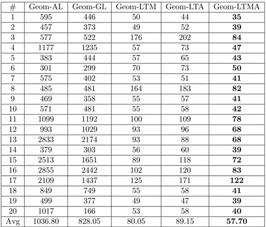
in-terval. The accuracy of the local search was set as δ = ε in the algorithms with the local improvement. Results of numerical experiments are reported in Tables 1.2–1.15 where the number of function trials executed until the satisfaction of the stopping rule is presented for each considered method (the best results for the methods within the same class are shown in bold).
The first series of numerical experiments was carried out with geome-tric and information algorithms without the local improvement on 20 test functions given in Appendix A. Parameters of the geometric methods Geom-AL, Geom-GL, Geom-LTM, Geom-LTA, and Geom-LTMA were chosen as follows. For the method Geom-AL, the estimates of the Lipschitz constants were computed as the maximum between the values calculated as relative dif-ferences on 10−7-grid and the values given in [83]. For the methods Geom-GL,
Geom-LTM, and Geom-LTMA, the reliability parameter r = 1.1 was used as recommended in [189]. The technical parameter ξ = 10−8 was used for
all the methods with the local tuning (LTM, LTA, and Geom-LTMA). For the method Geom-LTA, the parameter r was increased with the step equal to 0.1 starting from r = 1.1 until all 20 test problems were solved (i. e., for all the problems the algorithm stopped in the ε-neighborhood of a global minimizer: |xk− x∗| ≤ ε, where xk is the point generated at Step 6
of GS and x∗ is the global minimizer (known a priori for all test problems)).
This situation happened for r = 1.8: the corresponding results are shown in the column Geom-LTA of Table 1.2.
As can be seen from Table 1.2, the performance of the method Geom-LTMA was better with respect to the other geometric algorithms tested. The experiments also showed that the additive convolution (Geom-LTA) did
30 Univariate Lipschitz Global Optimization
# Geom-AL Geom-GL Geom-LTM Geom-LTA Geom-LTMA
1 595 446 50 44 35 2 457 373 49 52 39 3 577 522 176 202 84 4 1177 1235 57 73 47 5 383 444 57 65 43 6 301 299 70 73 50 7 575 402 53 51 41 8 485 481 164 183 82 9 469 358 55 57 41 10 571 481 55 58 42 11 1099 1192 100 109 78 12 993 1029 93 96 68 13 2833 2174 93 88 68 14 379 303 56 60 39 15 2513 1651 89 118 72 16 2855 2442 102 120 83 17 2109 1437 125 171 122 18 849 749 55 58 41 19 499 377 49 47 39 20 1017 166 53 58 40 Avg 1036.80 828.05 80.05 89.15 57.70
Table 1.2: Number of trials performed by the considered geometric methods without the local improvement on 20 tests from Appendix A.
not guarantee the proximity of the found solution to the global minimum with the common value r = 1.1. With an increased value of the reliability parameter r, the average number of trials performed by this method on 20 tests was also slightly worse than that of the method with the maximum convolution (Geom-LTM) but better than the averages of the methods using global estimates of the Lipschitz constants (Geom-AL and Geom-GL).
Results of numerical experiments with information methods without the local improvement techniques (methods Inf-AL, Inf-GL, Inf-LTM, Inf-LTA, and Inf-LTMA) on the same 20 tests from Appendix A are shown in Table 1.3. Parameters of the information methods were chosen as follows. The estimates of the Lipschitz constants for the method Inf-AL were the same as for the method Geom-AL. The reliability parameter r = 2 was used in the methods Inf-GL, Inf-LTM, and Inf-LTMA, as recommended in [189, 213, 215]. For all the information methods with the local tuning techniques (LTM, Inf-LTA, and Inf-LTMA), the value ξ = 10−8was used. For the method Inf-LTA,
Acceleration techniques in LGO 31 # Inf-AL Inf-GL Inf-LTM Inf-LTA Inf-LTMA
1 422 501 46 35 32 2 323 373 47 38 36 3 390 504 173 72 56 4 833 1076 51 56 47 5 269 334 59 47 37 6 208 239 65 46 45 7 403 318 49 38 37 8 157 477 163 113 63 9 329 339 54 48 42 10 406 435 51 42 38 11 773 1153 95 78 75 12 706 918 88 71 64 13 2012 1351 54 54 51 14 264 349 55 44 38 15 1778 1893 81 82 71 16 2023 1592 71 67 64 17 1489 1484 128 121 105 18 601 684 52 43 43 19 352 336 44 34 33 20 681 171 55 39 39 Avg 720.95 726.35 74.05 58.40 50.80
Table 1.3: Number of trials performed by the considered information methods without the local improvement on 20 tests from Appendix A.
the parameter r was increased (starting from r = 2) up to the value r = 2.3 when all 20 test problems were solved.
As can be seen from Table 1.3, the performance of the method Inf-LTMA was better (as also verified for its geometric counterpart) with respect to the other information algorithms tested. The experiments also showed that the average number of trials performed by the Inf-LTA method with r = 2.3 on 20 tests was better than that of the method with the maximum convolution (Inf-LTM).
The second series of experiments (see Table 1.4) was executed on the class of 100 Pint´er’s test functions from [153] with all geometric and information algorithms without the local improvement (i. e., all the methods used in the first series of experiments). Each Pint´er’s test function is defined over the interval [a, b] = [−5, 5] as follows:
32 Univariate Lipschitz Global Optimization
Method Average StDev Method Average StDev
Geom-AL 1080.24 91.17 Inf-AL 750.03 66.23
Geom-GL 502.17 148.25 Inf-GL 423.19 109.26
Geom-LTM 58.96 9.92 Inf-LTM 52.13 5.61
Geom-LTA 70.48 17.15 Inf-LTA 36.47 6.58
Geom-LTMA 42.34 6.63 Inf-LTMA 38.10 5.96
Table 1.4: Results of numerical experiments with the considered geometric and information methods without the local improvement on 100 Pint´er’s test functions from [153].
fn(x) = 0.025(x − x∗n)2+ sin2[(x − xn∗) + (x − x∗n)2] + sin2(x − x∗n), 1 ≤ n ≤ 100, (1.16)
where the global minimizer x∗n, 1 ≤ n ≤ 100, is chosen randomly and
diffe-rently for all functions from the search interval by means of the random num-ber generator used in the GKLS-generator of multidimensional test functi-ons (see [65] for details). The GKLS-generator can be free-downloaded, so the source code is available for repeating all the experiments with random functions. Parameters of the methods Geom-AL, Geom-GL, Geom-LTM, Geom-LTMA, and Inf-AL, Inf-GL, Inf-LTM and Inf-LTMA were the same as in the first experimental series (r = 1.1 for all the geometric methods and r = 2 for the information methods). The reliability parameter for the method Geom-LTA was increased from r = 1.1 to r = 1.8 (when all 100 problems were solved). All the information methods were able to solve all 100 test problems with r = 2 (see Table 1.4). The average performance of the Geom-LTMA and the Inf-LTA methods was the best among the other considered geometric and information algorithms, respectively.
In the following several series of experiments, the local improvement techniques were compared on the same sets of test functions. In the third series (see Table 1.5), six methods (geometric and information) with the op-timistic local improvement (methods LTIMO, LTIAO, Geom-LTIMAO and Inf-LTIMO, Inf-LTIAO and Inf-Geom-LTIMAO) were compared on the class of 20 test functions from [83] (see Appendix A). The reliability para-meter r = 1.1 was used for the methods Geom-LTIMO and Geom-LTIMAO and r = 2 was used for the method Inf-LTIMO. For the method Geom-LTIAO r was increased to 1.6 and for the methods Inf-LTIMAO and Inf-LTIAO r was increased to 2.3. As can be seen from Table 1.5, the best average result among all the algorithms was shown by the method Geom-LTIMAO (while the Inf-LTIMAO was the best in average among the considered information methods).
Acceleration techniques in LGO 33 # Geom LTIMO Geom LTIAO Geom LTIMAO Inf LTIMO Inf LTIAO Inf LTIMAO 1 45 41 35 47 35 37 2 47 49 35 45 37 41 3 49 45 39 55 45 51 4 47 53 43 49 53 53 5 55 49 47 51 47 47 6 51 49 45 47 43 47 7 45 45 39 49 37 39 8 37 41 35 41 45 47 9 49 51 41 51 51 40 10 47 49 41 51 43 43 11 49 53 45 55 59 55 12 43 53 35 53 67 45 13 51 53 57 41 51 55 14 45 45 43 49 43 45 15 45 57 47 45 55 53 16 49 55 53 47 49 53 17 93 53 95 59 55 53 18 45 47 37 49 41 44 19 45 43 35 46 33 35 20 43 45 37 49 35 39 Avg 49.00 48.80 44.20 48.95 46.20 46.10
Table 1.5: Number of trials performed by the considered geometric and in-formation methods with the optimistic local improvement on 20 tests from Appendix A.
34 Univariate Lipschitz Global Optimization # Geom LTIMP Geom LTIAP Geom LTIMAP Inf LTIMP Inf LTIAP Inf LTIMAP 1 49 46 36 47 38 35 2 49 50 38 47 37 35 3 165 212 111 177 56 57 4 56 73 47 51 56 46 5 63 66 48 57 47 38 6 70 71 51 64 46 45 7 54 53 41 51 39 38 8 157 182 81 163 116 99 9 53 57 43 52 52 43 10 56 59 42 52 43 39 11 100 114 77 95 78 72 12 93 97 69 87 73 64 13 97 86 68 55 52 50 14 58 197 43 60 46 42 15 79 120 76 79 82 70 16 97 115 81 71 66 60 17 140 189 139 127 129 100 18 55 60 42 51 42 42 19 52 50 36 46 33 32 20 54 56 40 51 37 40 Avg 79.85 97.65 60.45 74.15 58.40 52.35
Table 1.6: Number of trials performed by the considered geometric and in-formation methods with the pessimistic local improvement on 20 tests from Appendix A.
Acceleration techniques in LGO 35
Optimistic strategy Pessimistic strategy
Method r Average StDev Method r Average StDev
Geom-LTIMO 1.3 49.52 4.28 Geom-LTIMP 1.1 66.44 21.63 Geom-LTIAO 1.9 48.32 5.02 Geom-LTIAP 1.8 93.92 197.61 Geom-LTIMAO 1.4 45.76 5.83 Geom-LTIMAP 1.1 48.24 14.12 Inf-LTIMO 2.0 48.31 4.29 Inf-LTIMP 2.0 53.06 7.54 Inf-LTIAO 2.1 36.90 5.91 Inf-LTIAP 2.0 37.21 7.25 Inf-LTIMAO 2.0 38.24 6.36 Inf-LTIMAP 2.0 39.06 6.84 Table 1.7: Results of numerical experiments with the considered geome-tric and information methods with the local improvement techniques on 100 Pint´er’s test functions from [153].
In the fourth series of experiments, six methods (geometric and informa-tion) using the pessimistic local improvement were compared on the same 20 test functions. The obtained results are presented in Table 1.6. The usual values r = 1.1 and r = 2 were used for the geometric (Geom-LTIMP and Geom-LTIMAP) and the information (Inf-LTIMP and Inf-LTIMAP) met-hods, respectively. The values of the reliability parameter ensuring the so-lution to all the test problems in the case of methods Geom-LTIAP and Inf-LTIAP were set as r = 1.8 and r = 2.3, respectively. As can be seen from Table 1.6, the “Maximum” and the “Maximum-Additive” local tuning techniques were more stable and generally allowed us to find the global so-lution for all test problems without increasing r. Moreover, the methods Geom-LTIMAP and Inf-LTIMAP showed the best performance with respect to the other techniques in the same geometric and information classes, re-spectively.
In the fifth series of experiments, the local improvement techniques were compared on the class of 100 Pint´er’s functions. The obtained results are presented in Table 1.7. The values of the reliability parameter r for all the methods were increased, starting from r = 1.1 for the geometric methods and r = 2 for the information methods, until all 100 problems from the class were solved. It can be seen from Table 1.7, that the best average number of trials for both the optimistic and pessimistic strategies was almost the same (36.90 and 37.21 in the case of information methods and 45.76 and 48.24 in the case of geometric methods, for the optimistic and for the pessimistic strategies, respectively). However, the pessimistic strategy seemed to be more stable since its reliability parameter (needed to solve all the problems) generally remained smaller than that of the optimistic strategy. In average, the Geom-LTMA and the Inf-LTA methods was the best among the other considered geometric and information algorithms, respectively.
36 Univariate Lipschitz Global Optimization 20 40 60 80 100 120 140 160 180 0 10 20 30 40 50 60 70 80 90 100 Geom−GL Geom−LTM Geom−LTIMP Geom−LTMA Geom−LTIMAP (a) 20 40 60 80 100 120 140 160 180 0 10 20 30 40 50 60 70 80 90 100 Inf−GL Inf-LTM Inf-LTIMP Inf-LTMA Inf-LTIMAP (b)
Figure 1.2: Operational characteristics for the geometric (a) and informa-tion (b) Lipschitz global optimizainforma-tion algorithms over 100 Shekel-type test functions
Finally, in the sixth series of experiments, the following 10 methods have been compared on the class of 100 Shekel-type test functions: Geom-GL, Geom-LTM, Geom-LTIMP, Geom-LTMA, Geom-LTIMAP, Geom-GL, Inf-LTM, Inf-LTIMP, Inf-LTMA, Inf-LTIMAP. In this series of experiments, con-trol parameters for each algorithm have been set as follows. First, for each method the technical parameter ξ was set to 10−8. Second, for each method
the initial value r = 2 was used over all the classes of test functions and it was increased until all test problems were solved. Each test problem was considered to be solved if an algorithm has generated a point xkafter k trials
such that:
|xk− x∗| ≤ ǫ, (1.17)
where x∗ is the global minimizer for the problem (1.3),(1.2), and ǫ is the
given accuracy (that was set 10−6 in our experiments). So, for the algorithms
Geom-GL, Geom-LTM, and Geom-LTIMP r was set to 2, for Geom-LTMA – 2.5, for Geom-LTIMAP – 2.3, for Inf-GL – 2.8, for Inf-LTM – 3, for Inf-LTIM – 3.7, for Inf-LTMA – 4, and for Inf-LTIMAP – 4.2. However, it should be noticed that many test problems of the class can be solved also with smaller values of the parameter r for each algorithm. The use of a common value of the parameters for the whole class of test functions can increase the number of trials.
One of the most efficient methods for a numerical comparison on the class of test problems in terms of costly function evaluations uses operational characteristics proposed by Grishagin in [78]. The operational characteristic of a method on a class of test problems is a non-decreasing function that indicates the number of problems solved by this method after each trial (see the next Section for details). It is convenient to represent the operational characteristics of a method in a graph (see Fig. 1.2.a and Fig. 1.2.b). Among
Solving practical engineering problems 37 different methods the better method is that with the highest operational characteristic.
As we can see from Fig. 1.2, all the methods can be divided into three groups with respect to their performance: methods with the global estimate of the Lipschitz constant (methods Geom-GL and Inf-GL) with the lower operational characteristics, local tuning with local improvement (methods Geom-LTMP, Geom-LTIMAP, Inf-LTMP, and Inf-LTIMAP) with the hig-hest operational characteristics, and local tuning without local improvement (methods Geom-LTM, Geom-LTMA, Inf-LTM, and Inf-LTMA), that have the medium operational characteristics. Since the methods Geom-GL and Inf-GL use the global Lipschitz constants, they need more trials to achieve the desired accuracy as the Lipschitz constant can be large in few subintervals and small in other ones. That is the advantage of the local tuning techni-ques that use the local Lipschitz constants for each subinterval and avoid this problem. We can see also that the use of local improvement techniques improves the results also and a combination of the local tuning with the local improvement techniques can accelerate the search significantly.
Figure 1.2 demonstrates also that the methods with the “maximum-additive” local tuning show better performance with respect to the other techniques: among all geometric (information) algorithms over the presented class of test problems the best one was Geom-LTIMAP (Inf-LTIMAP) and among all geometric (information) algorithms without local tuning the best one was Geom-LTMA (Inf-LTMA).
1.2
Solving practical engineering problems
As mentioned above, univariate Lipschitz global optimization are very impor-tant from a practical engineering point of view. In this work, two practical engineering problems are considered. The first problem is the sinusoidal parameter estimation problem that is considered to fit a sum of damped si-nusoids to a series of noisy observations. It can be formulated as a nonlinear least-squares global optimization problem (see, e.g., [72, 73, 195]). A one-parametric case study is examined to determine an unknown frequency of a signal. The second problem is finding the minimal root of the non-linear equation. In this problem, a device whose behavior depends on some charac-teristic function φ(x) is considered. The device works correctly only if the value of f (x) is greater than zero. It is necessary to find the first point x for which the value of φ(x) is equal to zero or to demonstrate that φ(x) is positive over the whole search interval. Obviously, the value of φ(x) at the initial point x0 = 0 should be positive. This problem was reformulated as
38 Univariate Lipschitz Global Optimization the global optimization problem in [38, 188].
1.2.1
Applications in noisy data fitting and electrical
engineering
A general nonlinear regression model can be often considered in the form of fitting a sum of damped sinusoids to a series of observations corrupted by noise (see, e. g., [20, 27, 63, 73, 121]). The sinusoidal functions are fre-quently used in many real-life applications such as signal processing (see, e. g., [31, 48, 51, 71, 76, 131, 156]). Parameters x of these functions (consis-ting of amplitudes, frequencies, and phases) can be estimated by solving the following minimization problem:
f (x∗) = f∗ = min x∈Df (x), f (x) = T X i=1 (yti − φ(x, ti)) 2 , x ∈ D ⊂ Rn, (1.18) where φ(x, t) = s X l=1 aledltsin(2πωlt + θl), t = t1, . . . , tT, (1.19)
and s ≥ 1 is a fixed integer, x = (a, d, ω, θ) with a = (a1, . . . , as),
d = (d1, . . . , ds), ω = (ω1, . . . , ωs), and θ = (θ1, . . . , θs).
It is supposed that real-valued observations yti are affected by noise: yti = φ(¯x, ti) + ξti, i = 1, . . . , T, (1.20) where ¯x is the true vector of parameters (it coincides with the estimator x∗
from (1.18) in the case of noise-free observations) and ξti, i = 1, . . . , T , are independently and identically distributed random variables with zero mean and a given variance σ2.
As a case study to illustrate the performance of various techniques for solving the global optimization problem (1.18)–(1.20), let us consider the sine function with unknown frequency only in (1.19) (i. e., s = 1 and a1 =
1, d1 = 0, θ1 = 0 in (1.19)) over uniformly sampled observations yi, i =
1, . . . , T in (1.20). In this case, the vector of parameters x consists of only one component x := ω = ω1. In spite of its apparent simplicity, such a problem
is however representative from the practical point of view (see, e. g., [20, 63, 156]) and useful to obtain conclusions on the problem behavior that can be then generalized to a general multiparametric model (1.18)–(1.20).