Search for long-lived particles that decay into final states containing
two electrons or two muons in proton-proton collisions
at
p
ffiffis
¼ 8 TeV
V. Khachatryan et al.*(CMS Collaboration)
(Received 25 November 2014; published 18 March 2015)
A search is performed for long-lived particles that decay into final states that include a pair of electrons or a pair of muons. The experimental signature is a distinctive topology consisting of a pair of charged leptons originating from a displaced secondary vertex. Events corresponding to an integrated luminosity of 19.6ð20.5Þ fb−1in the electron (muon) channel were collected with the CMS detector at the CERN LHC in proton-proton collisions at pffiffiffis¼ 8 TeV. No significant excess is observed above standard model expectations. Upper limits on the product of the cross section and branching fraction of such a signal are presented as a function of the long-lived particle’s mean proper decay length. The limits are presented in an approximately model-independent way, allowing them to be applied to a wide class of models yielding the above topology. Over much of the investigated parameter space, the limits obtained are the most stringent to date. In the specific case of a model in which a Higgs boson in the mass range 125–1000 GeV=c2decays
into a pair of long-lived neutral bosons in the mass range 20–350 GeV=c2, each of which can then decay to
dileptons, the upper limits obtained are typically in the range 0.2–10 fb for mean proper decay lengths of the long-lived particles in the range 0.01–100 cm. In the case of the lowest Higgs mass considered (125 GeV=c2), the limits are in the range 2–50 fb. These limits are sensitive to Higgs boson branching
fractions as low as 10−4.
DOI:10.1103/PhysRevD.91.052012 PACS numbers: 14.80.Ec, 12.60.-i, 13.85.Rm
I. INTRODUCTION
Long-lived particles, which could manifest themselves through their delayed decays to leptons, are predicted in many extensions of the standard model (SM). For example, such particles could occur in supersymmetric (SUSY) scenarios such as “split SUSY” [1] or SUSY with very weak R-parity violation [2], “hidden valley” models [3], and the “minimal B− L extension of the standard model [4].”
In this paper we present an inclusive search for massive, long-lived exotic particles that decay to final states that include a pair of charged leptons using proton-proton (pp) collision data collected atpffiffiffis¼ 8 TeV during 2012 with the compact muon solenoid (CMS) detector at the CERN LHC. Specifically, we search for events containing a pair of electrons or muons (dileptons) originating from a common secondary vertex within the volume of the CMS tracker, and with a significant transverse displacement from the event primary vertex. This topological signature has the potential to provide clear evidence for physics beyond
the SM. Furthermore, it is almost free of background from SM processes.
The search results are formally obtained within the context of two specific models; however, they are presented in an approximately model-independent way, allowing them to be applied to a wide range of models in which long-lived particles decay to final states that include dileptons. In the first model, the long-lived particle is a spinless boson X, which has a nonzero branching fraction to dileptons. The X is pair-produced in the decay of a non-SM Higgs boson, H → XX, X → lþl− [5], where the
Higgs boson is produced through gluon-gluon fusion and l represents either an electron or a muon. In the second model, the long-lived particle is a neutralino ~χ0which can
decay via R-parity violating couplings into a neutrino and two charged leptons[2,6]. The neutralino is produced in events containing a pair of squarks, where a squark can decay via the process ~q → q~χ0; ~χ0→ lþl−ν. Both models
predict up to two displaced dilepton vertices per event in the CMS tracker volume, of which we only require one to be found. In this paper, we will use “LL particle” to refer to any long-lived particle, such as the X or ~χ0 particle
considered in our signal models.
The search presented here is an update of a previous CMS analysis that used a smaller data sample collected at
ffiffiffis p
¼ 7 TeV [7] in 2011. Improvements to the previous search include the higher integrated luminosity collected in 2012, which increases the sensitivity of the search, and an
* Full author list given at the end of the article.
Published by the American Physical Society under the terms of the Creative Commons Attribution 3.0 License. Further distri-bution of this work must maintain attridistri-bution to the author(s) and the published articles title, journal citation, and DOI.
improved analysis strategy, which substantially broadens the range of signal models to which the analysis is sensitive. The analysis complements two recent CMS publications: one searching for events that contain one electron and one muon from LL particle decays [8], and another that searches for LL particles decaying to dijets [9].
The D0 Collaboration has published the results of a search for leptons from nonprompt decays in its tracker volume [10,11], performed at pffiffiffis¼ 1.96 TeV at the Fermilab Tevatron. The ATLAS Collaboration has also performed related searches for long-lived particles using different decay channels [12,13], or lower-mass LL par-ticles[14], compared to those considered in this paper.
II. CMS DETECTOR
The central feature of the CMS apparatus is a super-conducting solenoid of 6 m internal diameter providing an axial field of 3.8 T. Within the field volume are a silicon pixel and strip tracker, a lead tungstate crystal electromag-netic calorimeter (ECAL), and a brass and scintillator hadron calorimeter. Muons are identified in gas-ionization detectors embedded in the steel flux-return yoke of the solenoid. A detailed description of the complete CMS detector, together with a definition of the coordinate system used and the relevant kinematic variables, can be found in Ref. [15].
The silicon tracker is composed of pixel detectors (three barrel layers, and two forward disks at both ends of the detector) surrounded by strip detectors (ten barrel layers, and three inner disks and nine forward disks at both ends of the detector). The tracker covers the pseudorapidity range jηj < 2.5. The pixel tracker and a subset of the strip tracker layers provide three-dimensional measurements of hit positions. The other strip tracker layers measure hit position only in (r, ϕ) in the barrel, or (z, ϕ) in the end cap. Taking advantage of the strong magnetic field and the high granularity of the silicon tracker, promptly produced charged particles with transverse momentum pT¼ 100 GeV=c are reconstructed with a resolution of
≈1.5% in pTand of≈15 μm in transverse impact parameter
d0. The track reconstruction algorithms [16] are able to
reconstruct displaced tracks with transverse impact param-eters up to ≈25 cm produced by particles decaying up to ≈50 cm from the beam line. The performance of the track reconstruction algorithms has been studied with simulated events[16]and data[17]. The silicon tracker is also used to reconstruct the primary vertex position with a precision of 10–12 μm in each dimension.
The ECAL consists of nearly 76 000 lead tungstate crystals, which provide coverage for jηj < 3. Its relative energy resolution improves with increasing energy. For energy deposits in the ECAL produced by electrons or photons of ET≈ 60 GeV, where ET¼ E sinðθÞ, the
reso-lution varies between 1.1% and 5% depending on their pseudorapidity [18]. Muons are measured in the range
jηj < 2.4 using detection planes based on three technolo-gies: drift tubes in the barrel region, cathode strip chambers in the end caps, and resistive-plate chambers in the barrel and end caps.
The first level of the CMS trigger system, composed of custom hardware processors, selects events of interest using information from the calorimeters and the muon detectors. A high-level trigger processor farm then employs the full event information to further decrease the event rate.
III. DATA AND SIMULATED SAMPLES Data from pp collisions at ffiffiffisp ¼ 8 TeV, corresponding to an integrated luminosity of 19.6 % 0.5 ð20.5% 0.5Þ fb−1, are used for the search in the electron (muon) channel. The lower effective luminosity in the electron channel is due to different data quality requirements for the relevant subdetectors compared to those in the muon channel.
The electron channel data are collected with a high-level trigger[19]that requires two clustered energy deposits in the ECAL. The leading (subleading) energy deposit is required to have transverse energy ET> 36ð22Þ GeV, and
both clusters are required to pass loose requirements on their compatibility with a photon/electron hypothesis. The muon channel trigger requires two muons, each recon-structed in the muon detectors without using any primary vertex constraint and having pT> 23 GeV=c. To suppress
muons from cosmic rays, the three-dimensional opening angle between the two muons must be less than 2.5 radians. Tracker information is not used in either trigger, as the track reconstruction algorithm used in the high-level trigger (as opposed to the standard offline track reconstruction) is not designed for finding displaced tracks.
For the H → XX model, simulated signal samples are generated using PYTHIA v6.426 [20] to simulate H
production through gluon-gluon fusion (gg → H). Subsequently, the H is forced to decay into XX, with the X bosons each decaying to dileptons (X → lþl−).
Several samples are generated with different combinations of the mass of the H (mH ¼ 125, 200, 400, 1000 GeV=c2)
and the mass of the X boson (mX¼ 20, 50, 150,
350 GeV=c2). The Higgs boson resonance is assumed to
be narrow for the purposes of simulation, but the impact of this assumption on the analysis is negligible. Furthermore, each sample is produced with three different X boson lifetimes corresponding to mean transverse decay lengths of approximately 2, 20, and 200 cm in the laboratory frame. For the ~χ0→ lþl−ν model, PYTHIA is used to simulate
squark pair production and subsequent decay to ~χ0, using
four combinations of squark and neutralino masses ðmq~; mχ~0Þ ¼ ð1500; 494Þ, (1000, 148), (350, 148), and
ð120; 48Þ GeV=c2. The R-parity violating couplings λ 122
and λ121are set to nonzero values to enable the decay of the
~
χ0 into two charged leptons and a neutrino. The values of
λ122 and λ121 are chosen to give a mean transverse decay
length of approximately 20 cm. The chosen masses explore the range to which CMS is currently sensitive.
Several simulated background samples are also gen-erated with PYTHIA. The dominant background is
Drell-Yan production of dileptons: prompt eþe− or μþμ− pairs
can be misidentified as displaced from the primary vertex due to detector resolution effects, and the production and decay of τþτ− pairs can produce genuinely displaced
leptons, although the probability that both τ leptons decay leptonically is small. Other simulated backgrounds are from t¯t, W=Z boson pair production (dibosons) with leptonic decays, and QCD multijet events. The last includes a potential background source from semileptonic decays of b=c-flavor hadrons. In all samples, the response of the detector is simulated using GEANT4
[21], and all the events are processed through the trigger emulation and event reconstruction chains of the CMS experiment.
IV. EVENT RECONSTRUCTION AND SELECTION To select pp collisions, events are required to contain a primary vertex with at least four associated tracks and a position displaced from the nominal interaction point by no more than 2 cm in the direction transverse to the beam, and no more than 24 cm in the direction along the beam. Furthermore, to reject events produced by the interaction of beam-related protons with the LHC collimators, for events with at least ten tracks, the fraction of tracks classified as “high purity,” as defined in Ref. [16], must exceed 25%. When more than one primary vertex is reconstructed in an event, we select the one with the largest sum of the p2
T of
the tracks associated to it.
In order to maximize the efficiency for reconstructing leptons from highly displaced vertices, we use lepton identification algorithms that are less stringent than the standard CMS algorithms, which are not needed to sup-press the very low backgrounds in this analysis. Leptons are identified using tracks reconstructed in the tracker that are classified as high purity, and have pseudorapidity jηj < 2. The latter requirement is imposed because the efficiency for finding tracks from displaced secondary vertices decreases at large jηj.
A track is identified as originating from an electron if its direction is consistent within a cone of size ΔR ¼
ffiffiffiffiffiffiffiffiffiffiffiffiffiffiffiffiffiffiffiffiffiffiffiffiffiffiffiffiffiffi ðΔηÞ2þ ðΔϕÞ2
p
< 0.1 with an energy deposit in the ECAL that is reconstructed as a photon. Here, Δη and Δϕ are the differences between the track and the energy deposit in the ECAL in η and ϕ, respectively. The energy of the electron is taken from the energy deposit in the ECAL, since it is less affected by bremsstrahlung loss than the measurement of the track pT. Additional quality
require-ments are placed on the ECAL energy deposit to reject background from hadronic sources.
A track is identified as originating from a muon if it matches a muon candidate found withinΔR < 0.1. Here, Δη and Δϕ are the differences in direction between the track and the muon found by the trigger in η and ϕ, respectively.
The LL particle candidates are formed from pairs of charged-lepton candidates. In the muon channel, the two tracks must each have pT> 26 GeV=c and be oppositely
charged. In the electron channel, the higher (lower) ET
electron must satisfy ET> 40 GeV (25 GeV). These
thresholds are set slightly higher than the corresponding trigger requirements to ensure that the selected events have high trigger efficiency. In the dielectron channel, the two tracks must also satisfy pT> 36 GeV=c (21 GeV=c) if
associated to the higher (lower) ET electron. This pT
requirement, which is slightly lower than the corresponding ET requirement placed on the ECAL energy deposit,
suppresses electrons that emit large amounts of brems-strahlung, and which thus tend to have poor impact parameter resolution. No charge requirement is applied to electrons, as the probability of mismeasuring the charge is non-negligible for high-pT electrons.
To reject promptly produced particles, the tracks are required to have a transverse impact parameter significance with respect to the primary vertex of jd0j=σd> 12, where
σdis the uncertainty on jd0j. This value is chosen to give an
expected background significantly below one event, which gives the best signal sensitivity for the vast majority of the LL particle lifetimes considered in this paper. Both lepton candidates are required to be isolated, to reject background from jets. Specifically, a hollow isolation cone is con-structed around each candidate, with a radius 0.04 <ΔR < 0.3 for electrons and 0.03 <ΔR < 0.3 for muons. Within this isolation cone, the ratio of the scalar P pTof all tracks
with pT> 1 GeV=c, excluding the other lepton candidate,
to the pTof the lepton, must be less than 0.1.
The two tracks are fitted to a common vertex, which is required to have χ2=dof < 10 ð5Þ in the electron (muon)
channel. To ensure that the candidate tracks were produced at this vertex, we require that the number of hits, between the center of CMS and the vertex position, that is assigned to the tracks is no more than 1, and that the number of missing hits on the tracks between the vertex position and the outer envelope of the tracker is no more than 3 (4) in the electron (muon) channel, where in both cases the numbers are summed over both tracks. A missing hit is defined as occurring when a track passes through an active sensor without being assigned a reconstructed hit. To eliminate background from J=ψ and ϒ decays, and from γ con-versions, LL particle candidates are required to have a dilepton invariant mass larger than 15 GeV=c2.
Cosmic ray muons may be reconstructed as back-to-back tracks. To reject them, the three-dimensional opening angle between the two muons must be less than 2.48 radians. This requirement is slightly tighter than the requirement in the
trigger. Background from misidentified leptons is reduced by requiring that the two lepton candidates are not both matched to the same trigger object or offline photon. Owing to the difficulty of modeling the low trigger efficiency for closely spaced muon pairs, the two muons are required to be separated by ΔR > 0.2.
Finally, the signed difference in azimuthal angles,ΔΦ, between the dilepton momentum vector, ¯pll, and the vector from the primary vertex to the dilepton vertex, ¯vll, is
required to satisfy jΔΦj < π=2, where ΔΦ is measured in the range 0 <ΔΦ < π. Dilepton candidates satisfying all other selection requirements, but with jΔΦj > π=2, are used to define a control region, as detailed in Sec. V.
Events containing at least one LL particle candidate that passes all selection requirements are accepted. Where more than one candidate is found in an event, the one with largest jd0j=σdis chosen. The jd0j=σdof a candidate is defined as
the minimum of the two jd0j=σdvalues of the leptons that
comprise it.
The overall signal efficiency is defined as the fraction of events in which at least one dilepton candidate passes all selection criteria. It is determined from the simulated signal samples, separately for the electron and muon channels, and independently for two different classes of events: first for events in which only one LL particle (X or ~χ0) decays to
the chosen lepton species, defining efficiency ϵ1, and
second for events in which both LL particles decay to the chosen lepton species, defining efficiency ϵ2. The
efficiencies are estimated for LL particle lifetimes corre-sponding to mean transverse decay lengths in the range of 200 μm–200 m, by reweighting the simulated signal events. The maximum value of ϵ1, which is attained for
H → XX with mH ¼ 1000 GeV=c2, mX ¼ 150 GeV=c2,
and cτ ¼ 1 cm, is approximately 36% (46%) in the electron (muon) channel, but it becomes significantly smaller at lower H masses or at longer and shorter lifetimes. For example, if cτ is increased to 20 cm for this set of masses, then ϵ1drops to 14% (20%) in the electron (muon)
channel. The efficiencies in the muon channel are generally higher because of the lower pTthresholds compared to the
corresponding thresholds in the electron channel.
In order to reduce the model dependence of our results, it is useful to define a set of acceptance criteria that specifies the LL particles decaying to dilepton final states that can be reconstructed in the CMS detector. Specifically, the gen-erated transverse decay length of the LL particle should be no more than 50 cm, and the generated electrons (muons) should satisfy the same ET(pT) and η requirements that are
applied to the reconstructed electrons (muons), which are listed earlier in this section. The acceptance A is defined as the fraction of LL particle decays that pass the acceptance criteria. Reevaluating the signal efficiency ϵ1, using only LL particle decays within the acceptance,
yields ϵ1=A, which is larger than ϵ1. For example, for
mH ¼ 1000 GeV=c2, mX ¼ 150 GeV=c2, and cτ ¼ 1 cm,
the value of ϵ1=A is approximately 44% (58%) in the
electron (muon) channel. More importantly, the efficiency defined in this way shows much less dependence on the choice of signal model; e.g. for this same choice of masses, but with cτ ¼ 20 cm, it falls only to 28% (40%) in the electron (muon) channel.
V. BACKGROUND ESTIMATION AND ASSOCIATED SYSTEMATIC UNCERTAINTIES
To estimate the background, we consider the quantities ¯
vll, ¯pllandΔΦ defined in Sec.IV. For signal events, ¯vll
corresponds to the flight direction of the LL particle, and assuming that the dilepton system produced when the LL particle decays is usually boosted with respect to its flight direction, the direction of ¯pllis correlated with that of ¯vll.
In contrast, for background events, ¯vlldoes not correspond
to the flight direction of any long-lived particle, so its angular distribution with respect to ¯pll should not show any forward-backward asymmetry. For example, in the case of Drell-Yan production of lþl−, ¯vll is determined only
by effects such as detector resolution or primary vertex misassignment. Although in the case of Drell-Yan produc-tion of τþτ−, leptonic products of the τ-lepton decays may
have significant values of jd0j=σd because of the nonzero
lifetime of the τ lepton, a vertex reconstructed from two such leptons would not correspond to a genuine particle decay vertex. Processes such as nonprompt J=ψ decay or γ conversions, which can give rise to genuine displaced dilepton vertices, are eliminated by the requirement on the minimum dilepton mass. Cosmic ray background is reduced to negligible levels via the dimuon opening angle requirement that rejects back-to-back muons.
Therefore if we define a signal region with jΔΦj < π=2 and a control region with jΔΦj > π=2, we expect that signal events will populate the former region, while back-ground events will be equally distributed between the two. Consequently, we can use the distribution of events in the control region to derive a data-driven estimate of the background expected in the signal region.
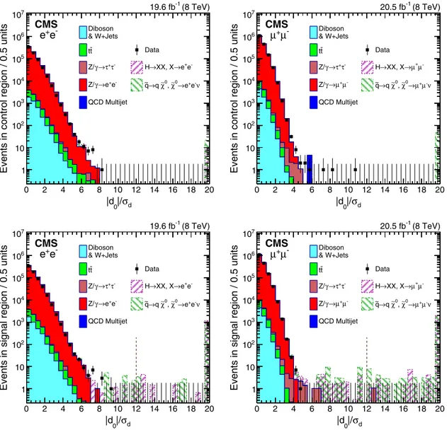
Figure1shows the jd0j=σddistribution of the simulated
events in the signal and control regions. Each of the simulated backgrounds is statistically consistent with being symmetrically divided between the two regions. The expected background is predominantly Drell-Yan dilepton production, with some contribution from QCD multijets. Any discrepancies between data and simulation are unim-portant since the analysis uses a data-driven background estimate. They may arise because of imperfect modeling in the simulation or because of the large statistical uncertainty in the simulated QCD multijet background. The multijet background near jd0j=σd¼ 6 in the top, right-hand plot
corresponds to a single simulated event. We observe that more than 97% (95%) of simulated signal events fall into the signal region for the X → lþl− (~χ0→ lþl−ν) model
for all the samples considered.
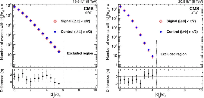
Besides using simulated events, we validate this method by comparing the jd0j=σd distribution in the signal region
with the one in the control region using data at jd0j=σd
values for which the sample is background dominated. Figure2shows the tail-cumulative distributions, which are defined as integrals from the plotted value to infinity, of jd0j=σd in the signal and control regions. However, the
region with jd0j=σd> 6 (4.5) in the electron (muon)
channel is excluded from the integral, to ensure that the signal region is background dominated. No statistically significant difference between the two regions is seen.
We observe zero events in data with jd0j=σd> 12 in the
control region, and this determines the probability distri-bution of the expected background level, as discussed in Sec. VII. The systematic uncertainty in this estimate is defined below.
Residual misalignment of the tracker is the only effect that can cause the expected background to differ signifi-cantly in the signal and control regions. This effect is largely removed by applying corrections, described below, to the conventionally signed [16] transverse and longi-tudinal (z0) impact parameters of all tracks. The mean offset
d σ |/ 0 |d 0 2 4 6 8 10 12 14 16 18 20
Events in control region / 0.5 units 1 10 2 10 3 10 4 10 5 10 6 10 7 10 & W+Jets Diboson tt -τ + τ → γ Z/ -e + e → γ Z/ QCD Multijet Data -e + e → XX, X → H ν -e + e → 0 χ∼ , 0 χ∼ q → q ~ -e + e (8 TeV) -1 19.6 fb CMS d σ |/ 0 |d 0 2 4 6 8 10 12 14 16 18 20
Events in control region / 0.5 units 1 10 2 10 3 10 4 10 5 10 6 10 7 10 & W+Jets Diboson tt -τ + τ → γ Z/ -µ + µ → γ Z/ QCD Multijet Data -µ + µ → XX, X → H ν -µ + µ → 0 χ∼ , 0 χ∼ q → q ~ -µ + µ (8 TeV) -1 20.5 fb CMS d σ |/ 0 |d 0 2 4 6 8 10 12 14 16 18 20
Events in signal region / 0.5 units 1
10 2 10 3 10 4 10 5 10 6 10 7 10 & W+Jets Diboson tt -τ + τ → γ Z/ -e + e → γ Z/ QCD Multijet Data -e + e → XX, X → H ν -e + e → 0 χ∼ , 0 χ∼ q → q ~ -e + e (8 TeV) -1 19.6 fb CMS d σ |/ 0 |d 0 2 4 6 8 10 12 14 16 18 20
Events in signal region / 0.5 units 1
10 2 10 3 10 4 10 5 10 6 10 7 10 & W+Jets Diboson tt -τ + τ → γ Z/ -µ + µ → γ Z/ QCD Multijet Data -µ + µ → XX, X → H ν -µ + µ → 0 χ∼ , 0 χ∼ q → q ~ -µ + µ (8 TeV) -1 20.5 fb CMS
FIG. 1 (color online). The jd0j=σddistribution for the electron (left) and muon (right) channels, shown in the top row for events in the
control region (jΔΦj > π=2) and in the bottom row for events in the signal region (jΔΦj < π=2). Of the two leptons forming a candidate, the distribution of the one with the smallest jd0j=σdis plotted. The solid points indicate the data, the shaded histograms are the simulated
background, and the hashed histograms show the simulated signal. The histogram corresponding to the H → XX model is shown for mH¼ 1000 GeV=c2and mX¼ 350 GeV=c2. The histogram corresponding to the ~χ0→ lþl−ν model is shown for m~q¼ 350 GeV=c2
and mχ~0¼ 140 GeV=c2. The background histograms are stacked, and each simulated signal sample is independently stacked on top of the total simulated background. The d0 corrections for residual tracker misalignment, discussed in the text, have been applied. The
vertical dashed line shows the selection requirement jd0j=σd> 12. Any entries beyond the right-hand side of a histogram are shown in
the last visible bin of the histogram.
from zero of the signed d0and z0of prompt muon tracks
(i.e. jd0j and jz0j below 500 μm) is measured as a function
of the track η and ϕ, and also as a function of run period. This bias, which arises from residual misalignment and is always less than 5 μm, is then subtracted from the measured impact parameters of individual tracks. To verify that this method is reliable, we first apply it to a data sample reconstructed with a preliminary alignment cali-bration, much inferior to the final alignment calibration used for the latest CMS data sets. In this sample, we observe a significant asymmetry between the control and signal regions, most of which disappears when the impact parameter corrections are applied.
Two approaches, described below, are used to assess the effect of any remaining systematic uncertainty in the background estimate due to misalignment. The first makes a direct measurement of the background asymmetry in the jd0j=σd distribution. The second checks how much, if at
all, the LL particle search results change if the impact parameter corrections are removed.
The first approach measures the systematic uncertainty remaining after the impact parameter corrections have been applied, by comparing the jd0j=σd distributions in the two
regions withΔΦ < 0 and ΔΦ > 0. Both signal and back-ground are expected to be equally divided between these two regions, so any significant asymmetry between them can only arise through systematic effects. We measure the size of this asymmetry by comparing the ratio of the number of events in the tail-cumulative distribution of jd0j=σd in the
region ΔΦ < 0 with that in the region ΔΦ > 0. Points at jd0j=σdvalues with very few events, such that the relative
statistical uncertainty in this ratio is greater than 30%, are excluded since they would not provide a precise estimate of the systematic uncertainty. The maximum difference of the ratio from unity for all remaining points is then taken to be the systematic uncertainty. Using this procedure, we obtain a systematic uncertainty of 11 and 21% in the electron and muon channels, respectively, in the estimated amount of background.
The second approach addresses a potential issue with the first method, namely that it measures the systematic uncertainty in the background normalization at lower values of jd0j=σd than are used in our standard selection.
In the data, the bias on the track d0due to misalignment is
less than 5 μm, whereas our jd0j=σd> 12 requirement
typically corresponds to a selection on jd0j of
approxi-mately 180 μm. This suggests that misalignment should not be a significant effect at large jd0j=σd. Nonetheless, to
allow for the possibility that it might be, we employ the second approach; namely, when computing our final limits, we do so twice, once with the impact parameter corrections applied, and once without them, and then take the worse limits as our final result. This should be conservative, given that as stated above, the impact parameter corrections remove the majority of any asymmetry caused by misalign-ment. In practice, the misalignment is so small that these two sets of limits are identical.
VI. SYSTEMATIC UNCERTAINTIES AFFECTING THE SIGNAL
The systematic effects influencing the signal efficiency arise from uncertainties in the efficiency of reconstructing > xd
σ|/ 0
Number of events with |d
1 10 2 10 3 10 4 10 5 10 6 10 -e + e /2) π | < Φ ∆ Signal (| /2) π | > Φ ∆ Control (| Excluded region (8 TeV) -1 19.6 fb CMS d σ |/ 0 |d 0 2 4 6 8 10 )σ Dif ference ( 0 2 > xd σ|/ 0
Number of events with |d
1 10 2 10 3 10 4 10 5 10 6 10 -µ + µ /2) π | < Φ ∆ Signal (| /2) π | > Φ ∆ Control (| Excluded region (8 TeV) -1 20.5 fb CMS d σ |/ 0 |d 0 2 4 6 8 10 )σ Dif ference ( -2 0
FIG. 2 (color online). Comparison of the tail-cumulative distributions of jd0j=σd for data in the signal region (jΔΦj < π=2) and the
control region (jΔΦj > π=2) for the electron channel (left) and the muon channel (right). The d0 corrections for residual tracker
misalignment, discussed in the text, have been applied. Of the two leptons forming a candidate, the distribution of the one with the smallest jd0j=σdis plotted. The bottom panels show the statistical significance of the difference between the distributions in the signal
and control regions.
tracks from displaced vertices, the trigger efficiency, the modeling of pileup (i.e. additional pp collisions in the same bunch crossing), the parton distribution function (PDF) sets, the renormalization and factorization scales used in generating simulated events, and the effect of higher-order QCD corrections.
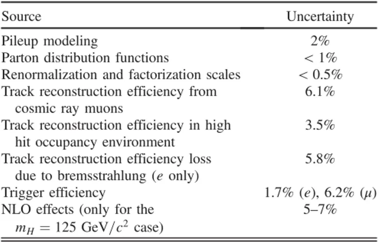
Table I summarizes the non-negligible sources of sys-tematic uncertainty affecting the signal efficiency. These
are discussed in more detail below. The most important sources are those related to the track reconstruction efficiency. The relative uncertainty in the measurement of the integrated luminosity is 2.6%[22].
Varying the modeling of the pileup within its estimated uncertainties yields a relative change in the signal selection efficiency of less than 2%, irrespective of the mass point chosen. The relative uncertainty due to the choice of PDF set is studied using the PDF4LHC prescription[23]and is less than 1% for all mass points. The dependence of the acceptance on the choice of the renormalization and factorization scales, which are chosen to be equal, is found to be well below 0.5% when they are varied by a factor of 0.5 or 2. These uncertainties are applied in the cross section limit calculation.
A. Track finding efficiency
Three methods are used to assess if the efficiency to reconstruct displaced tracks is correctly modeled by the simulation. The first method consists of a direct measure-ment of the efficiency to reconstruct isolated, displaced tracks, using cosmic ray muons. Events are selected from dedicated running periods with no beam present, and the cosmic ray muons are reconstructed by combining the hits in the muon detectors from opposite halves of the CMS detector. The efficiency to reconstruct, in the tracker, a track associated with a cosmic ray muon, as a function of the transverse and longitudinal impact parameters, is shown in Fig. 3. The systematic uncertainty on the dilepton
TABLE I. Systematic uncertainties affecting the signal effi-ciency over the two signal models and all mass values considered. In all cases, the uncertainty specified is a relative uncertainty. The next-to-leading-order (NLO) uncertainty is significant only for the H → XX model with mH¼ 125 GeV=c2. The relative
uncertainty in the integrated luminosity is 2.6%.
Source Uncertainty
Pileup modeling 2%
Parton distribution functions < 1%
Renormalization and factorization scales < 0.5% Track reconstruction efficiency from
cosmic ray muons 6.1%
Track reconstruction efficiency in high
hit occupancy environment 3.5%
Track reconstruction efficiency loss
due to bremsstrahlung (e only) 5.8%
Trigger efficiency 1.7% (e), 6.2% (μ)
NLO effects (only for the mH¼ 125 GeV=c2 case)
5–7%
Track reconstruction efficiency
0 0.2 0.4 0.6 0.8 1
Cosmic ray simulation Cosmic ray data
CMS | [cm] 0 |d 0 5 10 15 20 25 30 Simulation Data 0.6 0.8 1 1.2 1.4
Track reconstruction efficiency
0 0.2 0.4 0.6 0.8 1
Cosmic ray simulation Cosmic ray data
CMS | [cm] 0 |z 0 10 20 30 40 50 Simulation Data 0 0.5 1 1.5 2
FIG. 3 (color online). Efficiency to find a track in the tracker, measured using cosmic ray muons reconstructed in the muon detectors, as a function of the transverse (left) and longitudinal (right) impact parameters (relative to the nominal interaction point of CMS). The efficiency is plotted in bins of 2 cm width. For the left plot, the longitudinal impact parameter jz0j is required to be less than 10 cm, and
for the right plot, the transverse impact parameter jd0j must be less than 4 cm. The bottom panels show the ratio of the efficiency in data
to that in simulation. The uncertainties in the simulation are smaller than the size of the markers and are not visible.
efficiency is estimated as follows. We use the measured track reconstruction efficiency to estimate the efficiency to reconstruct a pair of leptons of given impact parameters. We then weight this efficiency according to the impact parameter distributions of the dileptons in the simulated signal Monte Carlo samples. The ratio of the estimated efficiency per dilepton candidate in data to simulation differs from unity by no more than 6.1% for any of the samples considered, so this value is taken as the systematic uncertainty.
A second method is used to study how the presence of a high density of tracker hits around displaced leptons degrades the track reconstruction performance. This method takes cosmic ray muon data, where each muon is recon-structed in the muon detectors and is successfully associated to a track reconstructed in the tracker. It embeds each of these tracks and its associated hits into a high-occupancy pp collision data event, and measures the fraction of these embedded tracks that can still be successfully reconstructed in this environment as a function of their impact parameters. The results are compared with those obtained by embedding tracks from simulated cosmic events in simulated pp collisions. The same procedure described at the end of the preceding paragraph is applied, and leads us to conclude that the efficiency per candidate has an additional systematic uncertainty, related to the track reconstruction efficiency in a high hit density environment, of 3.5%.
A third method[9]uses charged pions from K0
Sdecay to
establish that the track reconstruction efficiency is simu-lated with a relative systematic uncertainty of 5%. Since this method is mainly sensitive to the track reconstruction efficiency of low-pT hadrons in jets, it is used only to
provide additional reassurance that the displaced track reconstruction efficiency is well modeled.
These methods do not explicitly measure the track reconstruction efficiency for electrons, where an additional systematic uncertainty must be considered. For the leptons from LL particle decay in the simulated signal samples, the track reconstruction efficiency for the electrons is about 78% that of the muons, where the difference arises from the emission of bremsstrahlung. This difference does not show significant variation with respect to the transverse decay length of the LL particle. The material budget of the tracker is modeled in simulation to an accuracy of < 10% [24]. Since the amount of bremsstrahlung should be proportional to the amount of material in the tracker, this implies a corresponding relative uncertainty in the difference between the track reconstruction efficiencies for electrons and muons. This leads to a bremsstrahlung-related relative uncertainty in the tracking efficiency for electrons of 0.22 × 10%=ð1 − 0.22Þ ¼ 2.9%, where the denominator arises because this uncertainty is measured relative to the tracking efficiency for electrons, not muons. The corre-sponding systematic uncertainty for the dielectron candi-dates, which have two tracks, is twice as large, namely 5.8%.
B. Trigger efficiency
The trigger efficiency is measured using the “tag-and-probe” method[25]. In the muon channel, Z boson decays to dimuonsarereconstructedindatacollectedwithsingle-muon triggers. They are then used to measure the efficiency for a muon to pass the selection criteria of one leg of the dimuon trigger used in this analysis. The dimuon trigger efficiency is then obtained as the square of this single-muon efficiency, which assumes that there is no correlation in efficiency between the two leptons. This is generally a good assumption except for dimuons separated by ΔR < 0.2, which are excluded because the trigger is inefficient for closely spaced dimuons. In the electron channel, the method is similar, but since the two legs of the trigger for this channel have different ET thresholds, the efficiency of each leg is measured
separately. In data, the trigger efficiency is essentially 100% for electrons satisfying the analysis selection. Under the same conditions, the efficiency for muons with a pTof
about 26 GeV=c is above 70% and it reaches a plateau of approximately 85% for pT> 40 GeV=c.
The systematic uncertainty associated with the trigger efficiency is evaluated by taking the difference between the efficiency estimates from data and simulation, which yields a total relative uncertainty of 1.7% for the electron channel and 6.2% for the muon channel. To ensure that the trigger efficiencies obtained from the sample of Z bosons, in which the leptons are prompt, are also valid for leptons from LL particle decay, we examine the trigger efficiency in simu-lated signal events as a function of the lifetime of the LL particles. For LL particles passing the acceptance criteria defined in Sec.IV, no statistically significant dependence of the trigger efficiency on their lifetime is seen. Therefore, systematic uncertainties related to this source may be neglected in comparison to the systematic uncertainties on the trigger efficiency quoted above.
C. Effect of higher-order QCD corrections For the H → XX sample with mH ¼ 125 GeV=c2, the
leptons from the X boson decay have a combined efficiency of only a few percent for passing the lepton pTrequirements.
For this reason the signal efficiency at this mass is sensitive to the modeling of the Higgs boson pTspectrum, which may in
turn be influenced by higher-order QCD corrections. To evaluate this effect, we reweight the leading-order Higgs boson pT spectrum from our signal sample to match
the corresponding Higgs boson pT spectrum evaluated
at NLO [26–28]. For mH ¼ 125 GeV=c2 and mX ¼
20ð50Þ GeV=c2 the signal efficiency changes by 5%
(7%). This change is taken as an additional systematic uncertainty in the efficiency for the case mH ¼
125 GeV=c2. For the larger H masses that we consider,
and also for the neutralino channel, where a similar study was performed, the corresponding systematic uncertainty is below 0.5%, and hence neglected.
VII. RESULTS
Events from background sources are equally likely to populate the signal and control regions, whereas any events arising from LL particles will populate almost exclusively the signal region. In consequence, the presence of a signal in the data would reveal itself as a statistically significant excess of events in the signal region compared to the control region. After all selection requirements are applied, no events are found in the signal or control regions in either the electron or muon channel. There is thus no statistically significant excess. The jd0j=σddistributions of events in the
signal and control regions were shown in Fig.1.
We set 95% confidence level (C.L.) upper limits on the signal processes using the Bayesian method described in Ref.[29]. The limits are determined from a comparison of the number of events observed in the signal region with the number expected in the signal plus background hypothesis. The limit calculation takes into account the systematic uncertainties in the signal yield, described in Sec.VI, by introducing nuisance parameters for each of the uncertain-ties that are marginalized through an integration over their log-normal prior distributions. The expected number of background events μBin the control region, and hence also
in the signal region, is an additional nuisance parameter. It
[cm] τ c -3 10 10-2 10-1 1 10 102 103 104 105 ) [pb] - e + e → B(X XX) → (Hσ -3 10 -2 10 -1 10 1 10 2 10 (8 TeV) -1 19.6 fb CMS Observed limits 2 = 20 GeV/c X m 2 = 50 GeV/c X m ) σ 1 ± Expected limits ( 2 = 20 GeV/c X m 2 = 125 GeV/c H m [cm] τ c -3 10 10-2 10-1 1 10 102 103 104 105 ) [pb] - e + e → B(X XX) → (Hσ -3 10 -2 10 -1 10 1 10 (8 TeV) -1 19.6 fb CMS Observed limits 2 = 20 GeV/c X m 2 = 50 GeV/c X m ) σ 1 ± Expected limits ( 2 = 20 GeV/c X m 2 = 200 GeV/c H m [cm] τ c -2 10 10-1 1 10 102 3 10 104 ) [pb] - e + e → B(X XX) → (Hσ -4 10 -3 10 -2 10 -1 10 1 10 (8 TeV) -1 19.6 fb CMS Observed limits 2 = 20 GeV/c X m 2 = 50 GeV/c X m 2 = 150 GeV/c X m ) σ 1 ± Expected limits ( 2 = 20 GeV/c X m 2 = 400 GeV/c H m [cm] τ c -2 10 10-1 1 10 102 3 10 104 ) [pb] - e + e → B(X XX) → (Hσ -4 10 -3 10 -2 10 -1 10 1 10 2 10 (8 TeV) -1 19.6 fb CMS Observed limits 2 = 20 GeV/c X m 2 = 50 GeV/c X m 2 = 150 GeV/c X m 2 = 350 GeV/c X m ) σ 1 ± Expected limits ( 2 = 20 GeV/c X m 2 = 1000 GeV/c H m
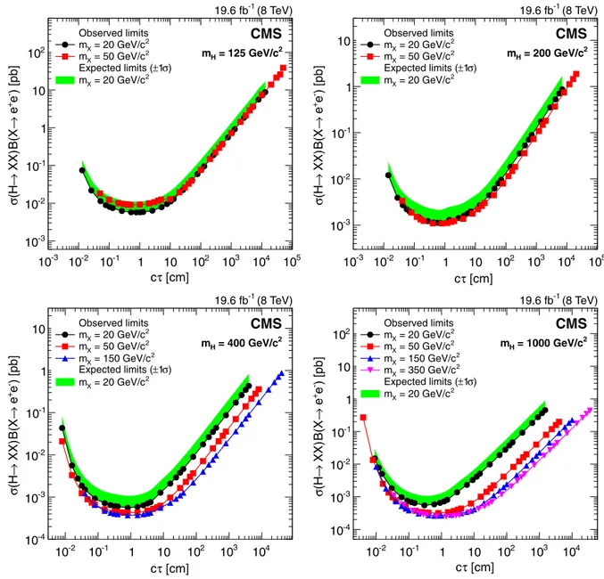
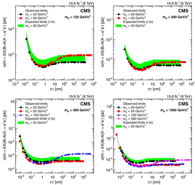
FIG. 4 (color online). The 95% C.L. upper limits on σðH → XXÞBðX → eþe−Þ, as a function of the mean proper decay length of the
X boson, for Higgs boson masses of 125 (top left), 200 (top right), 400 (bottom left), and 1000 GeV=c2(bottom right). In each plot,
results are shown for several X boson mass hypotheses. The shaded band shows the %1σ range of variation of the expected 95% C.L. limits for the case of a 20 GeV=c2X boson mass. Corresponding bands for the other X boson masses, omitted for clarity of presentation,
show similar agreement with the respective observed limits.
is constrained by the observed number of events NCin the
control region. Its probability distribution pðμBjNCÞ is
given by
pðμBjNCÞ ¼
μNC B
NC!expð−μBÞ;
as can be shown using Bayesian methodology assuming a flat prior in μB[29]. The expected background in the signal
region may differ from that in the control region, as a result of tracker misalignment. This is taken into account as described in Sec.V, by including an appropriate systematic
uncertainty, and by evaluating the limits twice, once with and once without correcting the track impact parameters for tracker misalignment, and taking the worse of these two sets of limits as the result.
If a genuine signal were present, it would give rise to an excess of events in the signal region with an expected number of
μS¼ Lσ½2Bð1 − BÞϵ1þ ϵ2B2'ð1 − fÞ; ð1Þ
where L is the integrated luminosity, ϵð1;2Þ are the signal efficiencies defined in Sec. IV, σ is the production cross section of H → XX (or ~q~q(þ ~q ~q) and B is the branching [cm] τ c -3 10 10-2 10-1 1 10 102 103 104 105 ) [pb] -µ + µ → B(X XX) → (Hσ -3 10 -2 10 -1 10 1 10 2 10 (8 TeV) -1 20.5 fb CMS Observed limits 2 = 20 GeV/c X m 2 = 50 GeV/c X m ) σ 1 ± Expected limits ( 2 = 20 GeV/c X m 2 = 125 GeV/c H m [cm] τ c -3 10 10-2 10-1 1 10 102 103 104 105 ) [pb] -µ + µ → B(X XX) → (Hσ -3 10 -2 10 -1 10 1 10 (8 TeV) -1 20.5 fb CMS Observed limits 2 = 20 GeV/c X m 2 = 50 GeV/c X m ) σ 1 ± Expected limits ( 2 = 20 GeV/c X m 2 = 200 GeV/c H m [cm] τ c -2 10 10-1 1 10 102 3 10 104 ) [pb] -µ + µ → B(X XX) → (Hσ -4 10 -3 10 -2 10 -1 10 1 10 (8 TeV) -1 20.5 fb CMS Observed limits 2 = 20 GeV/c X m 2 = 50 GeV/c X m 2 = 150 GeV/c X m ) σ 1 ± Expected limits ( 2 = 20 GeV/c X m 2 = 400 GeV/c H m [cm] τ c -2 10 10-1 1 10 102 3 10 104 ) [pb] - µ + µ → B(X XX) → (Hσ -4 10 -3 10 -2 10 -1 10 1 10 2 10 (8 TeV) -1 20.5 fb CMS Observed limits 2 = 20 GeV/c X m 2 = 50 GeV/c X m 2 = 150 GeV/c X m 2 = 350 GeV/c X m ) σ 1 ± Expected limits ( 2 = 20 GeV/c X m 2 = 1000 GeV/c H m
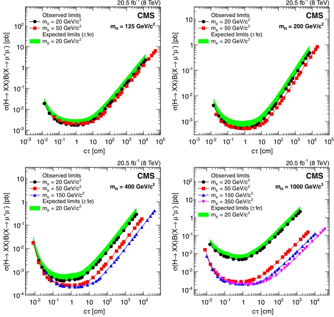
FIG. 5 (color online). The 95% C.L. upper limits on σðH → XXÞBðX → μþμ−Þ, as a function of the mean proper decay length of the
X boson, for Higgs boson masses of 125 (top left), 200 (top right), 400 (bottom left), and 1000 GeV=c2(bottom right). In each plot,
results are shown for several X boson mass hypotheses. The shaded band shows the %1σ range of variation of the expected 95% C.L. limits for the case of a 20 GeV=c2X boson mass. Corresponding bands for the other X boson masses, omitted for clarity of presentation,
show similar agreement with the respective observed limits.
fraction for the decay X → lþl− (or q → q~χ~ 0;
~
χ0→ lþl−ν). The parameter f is the mean number of
signal events expected to fall in the control region for each signal event in the signal region. This fraction is very small, being less than 3% for all the X → lþl− samples and less
than 5% for all the ~χ0→ lþl−ν samples considered here.
Its effect is to reduce slightly the effective signal efficiency, by causing some of the signal to be misinterpreted as background. One expects ϵ2≥ 1 − ð1 − ϵ1Þ2, where the
two terms are equal if the efficiency to select each of the two LL particles in an event is independent of the other, or the first term is larger if the presence of one LL particle increases the efficiency to select the other (as can happen if one lepton from each causes the event to trigger). Assuming ϵ2¼ 1 − ð1 − ϵ1Þ2, which is conservative since it
mini-mizes the value of μS, transforms Eq.(1) into
μS¼ 2LσBϵ1 " 1−1 2Bϵ1 # ð1 − fÞ: ð2Þ
Since μSin Eq.(2)depends not only on σB, but also on B,
the upper limits on σB depend on the assumed value of B, scaling approximately as the expression 1=½1 −1
2Bϵ1'. The
upper limits are thus best for low values of B, though the dependence of the limits on B is weak, particularly if ϵ1is
small. We set the value of B equal to unity in the expression in square brackets, so as to obtain conservative limits that are valid for any value of B.
For each combination of the H and X boson masses that is modeled, and for a range of mean proper decay lengths cτ of the X boson, 95% C.L. upper limits on
σðH → XXÞBðX → lþl−Þ are calculated. The observed
limits for the electron and muon channels are shown in Figs. 4 and 5, respectively. The less stringent limits for the muon channel in the mH¼ 1000 GeV=c2, mX ¼
20 GeV=c2 case are caused by low trigger efficiency
for nearby muons, and the consequent ΔR requirement. The corresponding limits on σð~q~q(þ ~q ~qÞBð~q → q~χ0;
~
χ0→ lþl−νÞ are shown in Fig. 6. The shaded band in
each of these plots shows the %1σ range of variation of the expected 95% C.L. limits, illustrated for one choice of masses. All the observed limits are consistent with the corresponding expected ones.
At pffiffiffis¼ 8 TeV, the theoretical cross sections for SM Higgs boson production through the dominant gluon-gluon fusion mechanism are 19.3, 7.1, 2.9, and 0.03 pb for Higgs boson masses of 125, 200, 400, and 1000 GeV=c2,
respectively[30]. The theoretical cross sections for ~q~q(þ
~
q ~q production are 2590, 10, 0.014, and 0.00067 pb for ~q masses of 120, 350, 1000, and 1500 GeV=c2, as evaluated
with thePROSPINOgenerator[31]assuming a gluino mass
of 5 TeV=c2. The observed limits on σB are usually well
below these theoretical cross sections, implying that non-trivial bounds are being placed on the decay modes involving LL particles, probing, for example, branching fractions as low as 10−4 and 10−6 in the Higgs and
supersymmetric models, respectively.
We also compute upper limits on the cross section times branching fraction within the acceptance A, where the latter is defined in the last paragraph of Sec. IV. Figures 7–8 show for the electron and muon channels, respectively, these limits on σðH → XXÞBðX → lþl−ÞAðX → lþl−Þ. [cm] τ c -1 10 1 10 102 103 ) [pb]ν - e + e → 0 χ∼ , 0 χ∼ q →q~ B() q~q~ +q~ q~( σ -4 10 -3 10 -2 10 -1 10 1 (8 TeV) -1 19.6 fb CMS Observed limits 2 = 120 / 48 GeV/c χ∼ / m q ~ m 2 = 350 / 148 GeV/c χ∼ / m q ~ m 2 = 1000 / 148 GeV/c χ∼ / m q ~ m 2 = 1500 / 494 GeV/c χ∼ / m q ~ m ) σ 1 ± Expected limits ( 2 = 120 / 48 GeV/c χ∼ / m q ~ m [cm] τ c -1 10 1 10 102 103 ) [pb]ν -µ + µ → 0 χ∼ , 0 χ∼ q →q~ B() q~q~ +q~ q~( σ -4 10 -3 10 -2 10 -1 10 1 (8 TeV) -1 20.5 fb CMS Observed limits 2 = 120 / 48 GeV/c χ∼ / m q ~ m 2 = 350 / 148 GeV/c χ∼ / m q ~ m 2 = 1000 / 148 GeV/c χ∼ / m q ~ m 2 = 1500 / 494 GeV/c χ∼ / m q ~ m ) σ 1 ± Expected limits ( 2 = 120 / 48 GeV/c χ∼ / m q ~ m
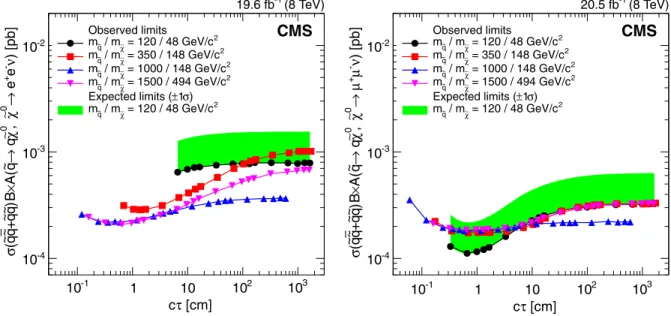
FIG. 6 (color online). The 95% C.L. upper limits on σð~q~q(þ ~q ~qÞBð~q → q~χ0; ~χ0→ lþl−νÞ for the electron (left), and muon (right)
channels, as a function of the mean proper decay length of the neutralino. The shaded band shows the %1σ range of variation of the expected 95% C.L. limits for the case of a 120 GeV=c2squark and a 48 GeV=c2neutralino mass. Corresponding bands for the other
squark and neutralino masses, omitted for clarity of presentation, show similar agreement with the respective observed limits.
Figure 9 shows the corresponding limits on σð~q~q(þ
~
q ~qÞBð~q → q~χ0; ~χ0 → lþl−νÞAð~q → q~χ0; ~χ0 → lþl−νÞ.
These limits restricted to the acceptance region show substantially less dependence on the Higgs boson and X boson masses and on the mean proper decay length cτ of the X boson. They are also less model dependent, as can be seen by the fact that the limits on σBA are similar for X → lþl− and ~χ0→ lþl−ν. The residual dependence of the
limits on cτ is due to the jd0j=σd> 12 requirement at small
values of cτ; whereas at larger values of cτ, it is caused by the fact that, even within the defined acceptance region, the tracking efficiency falls for leptons produced far from the beam line with very large impact parameters.
Although the limits described above are determined in the context of two specific models, the analysis is sensitive to any process in which an LL particle is produced and subsequently decays to a final state that includes dileptons. To place approximate limits on this more general class of models, one should use the limits within the acceptance region (i.e. on σBA), because of their smaller model dependence. In most signal models in which each event contains two identical LL particles that decay in this way, the limits on σBA shown in Figs. 7–9 should remain approximately valid. (The variation among the limit curves shown in these plots for different signal models and particle masses gives an indication of the accuracy of this
[cm] τ c -3 10 10-2 10-1 1 10 102 103 104 105 ) [pb] - e + e → A(X× B XX) → (Hσ -4 10 -3 10 -2 10 (8 TeV) -1 19.6 fb CMS Observed limits 2 = 20 GeV/c X m 2 = 50 GeV/c X m ) σ 1 ± Expected limits ( 2 = 20 GeV/c X m 2 = 125 GeV/c H m [cm] τ c -3 10 10-2 10-1 1 10 102 103 104 105 ) [pb] - e + e → A(X× B XX) → (Hσ -4 10 -3 10 -2 10 -1 10 (8 TeV) -1 19.6 fb CMS Observed limits 2 = 20 GeV/c X m 2 = 50 GeV/c X m ) σ 1 ± Expected limits ( 2 = 20 GeV/c X m 2 = 200 GeV/c H m [cm] τ c -2 10 10-1 1 10 102 3 10 104 ) [pb] - e + e → A(X× B XX) → (Hσ -4 10 -3 10 -2 10 -1 10 1 10 (8 TeV) -1 19.6 fb CMS Observed limits 2 = 20 GeV/c X m 2 = 50 GeV/c X m 2 = 150 GeV/c X m ) σ 1 ± Expected limits ( 2 = 20 GeV/c X m 2 = 400 GeV/c H m [cm] τ c -2 10 10-1 1 10 102 3 10 104 ) [pb] - e + e → A(X× B XX) → (Hσ -4 10 -3 10 -2 10 -1 10 1 10 2 10 (8 TeV) -1 19.6 fb CMS Observed limits 2 = 20 GeV/c X m 2 = 50 GeV/c X m 2 = 150 GeV/c X m 2 = 350 GeV/c X m ) σ 1 ± Expected limits ( 2 = 20 GeV/c X m 2 = 1000 GeV/c H m
FIG. 7 (color online). The 95% C.L. upper limits on σðH → XXÞBðX → eþe−ÞAðX → eþe−Þ, as a function of the mean proper decay
length of the X boson, for Higgs boson masses of 125 (top left), 200 (top right), 400 (bottom left), and 1000 GeV=c2(bottom right). In
each plot, results are shown for several X boson mass hypotheses. The shaded band shows the %1σ range of variation of the expected 95% C.L. limits for the case of a 20 GeV=c2X boson mass. Corresponding bands for the other X boson masses, omitted for clarity of
presentation, show similar agreement with the respective observed limits.
statement.) Exceptions could arise for models that give poor efficiency within the acceptance criteria, e.g. for models in which the leptons are not isolated; have impact parameters with significance below jd0j=σd< 12,
corre-sponding to jd0j ≲ 180 μm; are almost collinear with each
other (with the dilepton mass below 15 GeV=c2, or for the
muon channel ΔR < 0.2); or do not usually satisfy the jΔΦj < π=2 criterion, such that the parameter f becomes large (e.g. if the LL particle is slow moving and decays to many particles).
In models where each event contains only one LL particle that can decay inclusively to dileptons, the expected number of selected signal events for given σB
will be up to a factor of two lower, and so the limits on σBA will be up to a factor of two worse than those shown in Figs.7–9.
The acceptance A for any given model can be determined with a generator-level simulation, allowing limits on σBA to be converted to limits on σB. The following example illustrates this. The limits on σðH → XXÞBðX → lþl−Þ
quoted above are for H bosons produced through gluon-gluon fusion. If the H bosons were instead produced by the sum of all SM production mechanisms, their momentum spectra would be slightly harder. For mH ¼ 125 GeV=c2,
the acceptance would then be larger by a factor of approximately 1.18 (1.12) for mX ¼ 20 ð50Þ GeV=c2, with [cm] τ c -3 10 10-2 10-1 1 10 102 103 104 105 ) [pb] -µ + µ → A(X× B XX) → (Hσ -4 10 -3 10 -2 10 (8 TeV) -1 20.5 fb CMS Observed limits 2 = 20 GeV/c X m 2 = 50 GeV/c X m ) σ 1 ± Expected limits ( 2 = 20 GeV/c X m 2 = 125 GeV/c H m [cm] τ c -3 10 10-2 10-1 1 10 102 103 104 105 ) [pb] -µ + µ → A(X× B XX) → (Hσ -4 10 -3 10 -2 10 -1 10 (8 TeV) -1 20.5 fb CMS Observed limits 2 = 20 GeV/c X m 2 = 50 GeV/c X m ) σ 1 ± Expected limits ( 2 = 20 GeV/c X m 2 = 200 GeV/c H m [cm] τ c -2 10 10-1 1 10 102 3 10 104 ) [pb] -µ + µ → A(X× B XX) → (Hσ -4 10 -3 10 -2 10 -1 10 1 10 (8 TeV) -1 20.5 fb CMS Observed limits 2 = 20 GeV/c X m 2 = 50 GeV/c X m 2 = 150 GeV/c X m ) σ 1 ± Expected limits ( 2 = 20 GeV/c X m 2 = 400 GeV/c H m [cm] τ c -2 10 10-1 1 10 102 3 10 104 ) [pb] -µ + µ → A(X× B XX) → (Hσ -4 10 -3 10 -2 10 -1 10 1 10 2 10 (8 TeV) -1 20.5 fb CMS Observed limits 2 = 20 GeV/c X m 2 = 50 GeV/c X m 2 = 150 GeV/c X m 2 = 350 GeV/c X m ) σ 1 ± Expected limits ( 2 = 20 GeV/c X m 2 = 1000 GeV/c H m
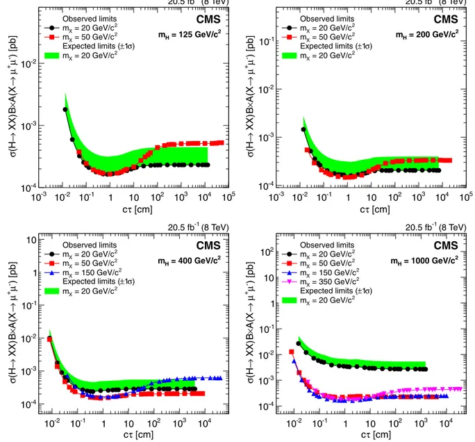
FIG. 8 (color online). The 95% C.L. upper limits on σðH → XXÞBðX → μþμ−ÞAðX → μþμ−Þ, as a function of the mean proper decay
length of the X boson, for Higgs boson masses of 125 (top left), 200 (top right), 400 (bottom left), and 1000 GeV=c2(bottom right). In
each plot, results are shown for several X boson mass hypotheses. The shaded band shows the %1σ range of variation of the expected 95% C.L. limits for the case of a 20 GeV=c2X boson mass. Corresponding bands for the other X boson masses, omitted for clarity of
presentation, show similar agreement with the respective observed limits.
a corresponding improvement in the limits on σB. The change is smaller for larger H boson masses.
VIII. SUMMARY
A search has been performed, using proton-proton collision data collected at pffiffiffis¼ 8 TeV, for long-lived particles that decay to a final state that includes a pair of electrons or a pair of muons. No such events have been seen. Quantitative limits have been placed on the product of the cross section and branching fraction of such a signal in the context of two specific models. In the first model, a Higgs boson, in the mass range 125–1000 GeV=c2, decays
into a pair of hypothetical, long-lived neutral bosons in the mass range 20–350 GeV=c2, each of which can decay to
dileptons. The upper limits obtained are typically in the range 0.2–10 fb for long-lived particles with mean proper decay lengths in the range 0.01–100 cm, and weaken to 250 fb for the lowest considered Higgs mass of 125 GeV=c2. In the second model, based on R-parity violating supersymmetry, a pair of squarks each decays to a quark and a long-lived neutralino ~χ0; the neutralino can
subsequently decay to eþe−ν or μþμ−ν. In this case, the
upper limits are typically in the range 0.2–5 fb for ~χ0mean
proper decay lengths in the range 0.1–100 cm and squark masses above 350 GeV=c2. For a lower squark mass of
120 GeV=c2, the limits are typically a factor of ten weaker.
These limits are sensitive to branching fractions as low as 10−4 and 10−6 in the Higgs boson and supersymmetric models, respectively. To allow the results to be reinterpreted in the context of other models, limits that are restricted to
the detector acceptance are also presented, reducing the model dependence. Over much of the investigated param-eter space, these limits are the most stringent to date.
ACKNOWLEDGMENTS
We congratulate our colleagues in the CERN accelerator departments for the excellent performance of the LHC and thank the technical and administrative staffs at CERN and at other CMS institutes for their contributions to the success of the CMS effort. In addition, we gratefully acknowledge the computing centers and personnel of the Worldwide LHC Computing Grid for delivering so effectively the computing infrastructure essential to our analyses. Finally, we acknowledge the enduring support for the construction and operation of the LHC and the CMS detector provided by the following funding agencies: BMWFW and FWF (Austria); FNRS and FWO (Belgium); CNPq, CAPES, FAPERJ, and FAPESP (Brazil); MES (Bulgaria); CERN; CAS, MoST, and NSFC (China); COLCIENCIAS (Colombia); MSES and CSF (Croatia); RPF (Cyprus); MoER, ERC IUT and ERDF (Estonia); Academy of Finland, MEC, and HIP (Finland); CEA and CNRS/ IN2P3 (France); BMBF, DFG, and HGF (Germany); GSRT (Greece); OTKA and NIH (Hungary); DAE and DST (India); IPM (Iran); SFI (Ireland); INFN (Italy); MSIP and NRF (Republic of Korea); LAS (Lithuania); MOE and UM (Malaysia); CINVESTAV, CONACYT, SEP, and UASLP-FAI (Mexico); MBIE (New Zealand); PAEC (Pakistan); MSHE and NSC (Poland); FCT (Portugal); JINR (Dubna); MON, RosAtom, RAS and RFBR (Russia);
[cm] τ c -1 10 1 10 102 103 ) [pb]ν - e + e → 0 χ∼ , 0 χ∼ q →q~ A(× B) q~q~ +q~ q~( σ 10-4 -3 10 -2 10 (8 TeV) -1 19.6 fb CMS Observed limits 2 = 120 / 48 GeV/c χ∼ / m q ~ m 2 = 350 / 148 GeV/c χ∼ / m q ~ m 2 = 1000 / 148 GeV/c χ∼ / m q ~ m 2 = 1500 / 494 GeV/c χ∼ / m q ~ m ) σ 1 ± Expected limits ( 2 = 120 / 48 GeV/c χ∼ / m q ~ m [cm] τ c -1 10 1 10 102 103 ) [pb]ν -µ + µ → 0 χ∼ , 0 χ∼ q →q~ A(× B) q~q~ +q~ q~( σ 10-4 -3 10 -2 10 (8 TeV) -1 20.5 fb CMS Observed limits 2 = 120 / 48 GeV/c χ∼ / m q ~ m 2 = 350 / 148 GeV/c χ∼ / m q ~ m 2 = 1000 / 148 GeV/c χ∼ / m q ~ m 2 = 1500 / 494 GeV/c χ∼ / m q ~ m ) σ 1 ± Expected limits ( 2 = 120 / 48 GeV/c χ∼ / m q ~ m
FIG. 9 (color online). The 95% C.L. upper limits on σð~q~q(þ ~q ~qÞBð~q → q~χ0; ~χ0→ lþl−νÞAð~q → q~χ0; ~χ0→ lþl−νÞ for the
electron (left), and muon (right) channels, as a function of the mean proper decay length of the neutralino. The shaded band shows the %1σ range of variation of the expected 95% C.L. limits for the case of a 120 GeV=c2 squark and a 48 GeV=c2 neutralino mass.
Corresponding bands for the other squark and neutralino masses, omitted for clarity of presentation, show similar agreement with the respective observed limits.
MESTD (Serbia); SEIDI and CPAN (Spain); Swiss Funding Agencies (Switzerland); MST (Taipei); ThEPCenter, IPST, STAR and NSTDA (Thailand); TUBITAK and TAEK (Turkey); NASU and SFFR (Ukraine); STFC (United Kingdom); DOE and NSF (USA). Individuals have received support from the Marie Curie program and the European Research Council and EPLANET (European Union); the Leventis Foundation; the A. P. Sloan Foundation; the Alexander von Humboldt Foundation; the Belgian Federal Science Policy Office; the Fonds pour la Formation à la Recherche dans l’Industrie et dans l’Agriculture (FRIA Belgium); the
Agentschap voor Innovatie door Wetenschap en Technologie (IWT Belgium); the Ministry of Education, Youth and Sports (MEYS) of the Czech Republic; the Council of Science and Industrial Research, India; the HOMING PLUS program of Foundation for Polish Science, cofinanced by the European Union, Regional Development Fund; the Compagnia di San Paolo (Torino); the Consorzio per la Fisica (Trieste); MIUR Grant No. 20108T4XTM (Italy); the Thalis and Aristeia programmes cofinanced by EU-ESF and the Greek NSRF; and the National Priorities Research Program by Qatar National Research Fund.
[1] J. L. Hewett, B. Lillie, M. Masip, and T. G. Rizzo, Sig-natures of long-lived gluinos in split supersymmetry,J. High Energy Phys. 09 (2004) 070.
[2] R. Barbier, C. Bérat, M. Besançon, M. Chemtob, A. Deandrea, E. Dudas, P. Fayet, S. Lavignac, G. Moreau, E. Perez, and Y. Sirois, R-parity violating supersymmetry, Phys. Rep. 420, 1 (2005).
[3] T. Han, Z. Si, K. M. Zurek, and M. J. Strassler, Phenom-enology of hidden valleys at hadron colliders, J. High Energy Phys. 07 (2008) 008.
[4] L. Basso, A. Belyaev, S. Moretti, and C. H. Shepherd-Themistocleous, Phenomenology of the minimal B− L extension of the standard model: Z0 and neutrinos,Phys. Rev. D 80, 055030 (2009).
[5] M. J. Strassler and K. M. Zurek, Discovering the Higgs through highly-displaced vertices,Phys. Lett. B 661, 263 (2008).
[6] B. C. Allanach, M. A. Bernhardt, H. K. Dreiner, C. H. Kom, and P. Richardson, Mass spectrum in R-parity violating minimal supergravity and benchmark points,Phys. Rev. D 75, 035002 (2007).
[7] CMS Collaboration, Search in leptonic channels for heavy resonances decaying to long-lived neutral particles,J. High Energy Phys. 02 (2013) 085.
[8] CMS Collaboration, Search for Displaced Supersymmetry in Events with an Electron and a Muon with Large Impact Parameters,Phys. Rev. Lett. 114, 061801 (2015). [9] CMS Collaboration, Search for long-lived neutral particles
decaying to dijets,Phys. Rev. D 91, 012007 (2015). [10] V. M. Abazov et al. (D0 Collaboration), Search for Neutral,
Long-Lived Particles Decaying into Two Muons in p ¯p Collisions atpffiffiffis¼ 1.96 TeV,Phys. Rev. Lett. 97, 161802 (2006).
[11] V. M. Abazov et al. (D0 Collaboration), Search for Long-Lived Particles Decaying into Electron or Photon Pairs with the D0 Detector, Phys. Rev. Lett. 101, 111802 (2008).
[12] ATLAS Collaboration, Search for A Light Higgs Boson Decaying to Long-Lived Weakly-Interacting Particles in Proton-Proton Collisions atpffiffiffis¼ 7 TeV with the ATLAS Detector,Phys. Rev. Lett. 108, 251801 (2012).
[13] ATLAS Collaboration, Search for long-lived, heavy par-ticles in final states with a muon and multi-track displaced vertex in proton-proton collisions atpffiffiffis¼ 7 TeV with the ATLAS detector,Phys. Lett. B 719, 280 (2013).
[14] ATLAS Collaboration, Search for long-lived neutral par-ticles decaying into lepton jets in proton–proton collisions at
ffiffiffis p
¼ 8 TeV with the ATLAS detector, J. High Energy Phys. 11 (2014) 088.
[15] CMS Collaboration, The CMS experiment at the CERN LHC,J. Instrum. 3, S08004 (2008).
[16] S. Chatrchyan et al. (CMS Collaboration), Description and performance of track and primary-vertex reconstruction with the CMS tracker,J. Instrum. 9, P10009 (2014). [17] CMS Collaboration, CMS tracking performance results
from early LHC operation,Eur. Phys. J. C 70, 1165 (2010). [18] CMS Collaboration, Energy calibration and resolution of
the CMS electromagnetic calorimeter in pp collisions at ffiffiffis
p
¼ 7 TeV,J. Instrum. 8, P09009 (2013).
[19] CMS Collaboration, Observation of the diphoton decay of the Higgs boson and measurement of its properties, Eur. Phys. J. C 74, 3076 (2014).
[20] T. Sjöstrand, S. Mrenna, and P. Z. Skands, PYTHIA 6.4 physics and manual,J. High Energy Phys. 05 (2006) 026. [21] S. Agostinelli et al. (GEANT4 Collaboration), GEANT4—a simulation toolkit,Nucl. Instrum. Methods Phys. Res., Sect. A 506, 250 (2003).
[22] CMS Collaboration, CMS luminosity based on pixel cluster counting—Summer 2013 update, Report No. CMS-PAS-LUM-13-001, 2013,http://cdsweb.cern.ch/record/1598864. [23] D. Bourilkov, R. C. Group, and M. R. Whalley, LHAPDF: PDF use from the Tevatron to the LHC, arXiv:hep-ph/ 0605240.
[24] CMS Collaboration, Studies of tracker material, Report No. CMS-PAS-TRK-10-003, 2010, http://cdsweb.cern.ch/ record/1279138.
[25] CMS Collaboration, Measurements of inclusive W and Z cross sections in pp collisions at pffiffiffis¼ 7 TeV, J. High Energy Phys. 01 (2011) 080.
[26] P. Nason, A new method for combining NLO QCD with shower Monte Carlo algorithms, J. High Energy Phys. 11 (2004) 040.