Soil Erosion Estimate in Southern Latium (Central Italy) Using RUSLE and Geostatistical Techniques

SOIL EROSION ESTIMATE IN SOUTHERN LATIUM

(CENTRAL ITALY) USING RUSLE AND GEOSTATISTICAL

TECHNIQUES

S. GRAUSO

ENEA – Dipartimento Sostenibilità dei Sistemi Produttivi e Territoriali

Divisione Modelli e tecnologie per la riduzione degli impatti antropici e dei rischi naturali Laboratorio Ingegneria sismica e prevenzione dei rischi naturali

Centro Ricerche Casaccia, Roma V. VERRUBBI, A. ZINI, A. PELOSO

ENEA – Dipartimento Sostenibilità dei Sistemi Produttivi e Territoriali

Divisione Modelli e tecnologie per la riduzione degli impatti antropici e dei rischi naturali Laboratorio Ingegneria sismica e prevenzione dei rischi naturali

Centro Ricerche Frascati, Roma C. CROVATO

ENEA – Dipartimento Sostenibilità dei Sistemi Produttivi e Territoriali Divisione Protezione e valorizzazione del territorio e del capitale naturale

Laboratorio Biogeochimica ambientale Centro Ricerche Casaccia, Roma

M. SCIORTINO

ENEA – Dipartimento Sostenibilità dei Sistemi Produttivi e Territoriali

Divisione Modelli e tecnologie per la riduzione degli impatti antropici e dei rischi naturali Laboratorio Modellistica climatica e impatti

Centro Ricerche Casaccia, Roma

AGENZIA NAZIONALE PER LE NUOVE TECNOLOGIE, L’ENERGIA E LO SVILUPPO ECONOMICO SOSTENIBILE

SOIL EROSION ESTIMATE IN SOUTHERN LATIUM

(CENTRAL ITALY) USING RUSLE AND GEOSTATISTICAL

TECHNIQUES

ENEA – Dipartimento Sostenibilità dei Sistemi Produttivi e Territoriali

Divisione Modelli e tecnologie per la riduzione degli impatti antropici e dei rischi naturali Laboratorio Ingegneria sismica e prevenzione dei rischi naturali

Centro Ricerche Casaccia, Roma V. VERRUBBI, A. ZINI, A. PELOSO

ENEA – Dipartimento Sostenibilità dei Sistemi Produttivi e Territoriali

Divisione Modelli e tecnologie per la riduzione degli impatti antropici e dei rischi naturali Laboratorio Ingegneria sismica e prevenzione dei rischi naturali

Centro Ricerche Frascati, Roma C. CROVATO

ENEA – Dipartimento Sostenibilità dei Sistemi Produttivi e Territoriali Divisione Protezione e valorizzazione del territorio e del capitale naturale

Laboratorio Biogeochimica ambientale Centro Ricerche Casaccia, Roma

M. SCIORTINO

ENEA – Dipartimento Sostenibilità dei Sistemi Produttivi e Territoriali

Divisione Modelli e tecnologie per la riduzione degli impatti antropici e dei rischi naturali Laboratorio Modellistica climatica e impatti

Centro Ricerche Casaccia, Roma

I contenuti tecnico-scientifici dei rapporti tecnici dell'ENEA rispecchiano l'opinione degli autori e non necessariamente quella dell'Agenzia.

The technical and scientific contents of these reports express the opinion of the authors but not necessarily the opinion of ENEA.

I Rapporti tecnici sono scaricabili in formato pdf dal sito web ENEA alla pagina http://www.enea.it/it/produzione-scientifica/rapporti-tecnici

SOIL EROSION ESTIMATE IN SOUTHERN LATIUM (CENTRAL ITALY) USING RUSLE AND GEOSTATISTICAL TECHNIQUES

S. GRAUSO, V. VERRUBBI, A. ZINI, A. PELOSO, C. CROVATO, M. SCIORTINO

Abstract

The present work aims to provide an assessment of soil erosion by means of the RUSLE model combined with different interpolation methods, in a Region of Italy where soil information is lacking and soil erosion risk is overlooked in land policies. The work concerns an area 4,000 km2 _{wide in the southern part of Latium (central Italy) and is based on}

simplified procedures for RUSLE factors calculation and on available rainfall, soil, land-cover and elevation data archives. The model results are shown in a map displaying that most of the area is characterized by very low or negligible soil erosion rates, on the average. Major soil loss affects areas on the central mountain ridge and inland areas with strong relief. On the average, the soil loss rate amounts to 44.4 Mg ha-1 _year-1_{. Given the lack of field}

observations to validate the modelled erosion rates, the map just can give an idea of the potential impact of erosion processes. Notwithstanding this limitation, the present work can support policy making in regional management and planning. The map will be updated once new information and details will be available.

Keywords: soil, erosion, spatial interpolation, GIS.

STIMA DELL'EROSIONE DEL SUOLO NEL LAZIO MERIDIONALE MEDIANTE IL MODELLO RUSLE E TECNICHE DI INTERPOLAZIONE GEOSTATISTICA

Riassunto

Il Lazio risulta ancora carente nell'informazione pedologica. Nonostante la frammentarietà dei dati tuttora disponibili, col presente lavoro abbiamo inteso testare l'operabilità del modello RUSLE e di alcune tecniche di interpolazione e simulazione geostatistica nell'area del Lazio meridionale p.p., per un'estensione areale di circa 4000 km2_{, nella}

prospettiva di poter estendere la stessa metodologia all'intera regione e contribuire alla messa a punto di strumenti conoscitivi utili per la pianificazione regionale. Il lavoro si è basato su dati pluviometrici, pedologici, plano-altimetrici e di uso e copertura del suolo contenuti in pubblicazioni scientifiche e database disponibili sul web. È stata anche condotta una campagna speditiva di campionamento dei suoli nell'area dei monti Lepini, Ausoni ed Aurunci al fine di colmare la carenza di dati in quell'area. La carta finale della perdita di suolo, intesa come valore medio su scala pluriennale, ottenuta dalla combinazione dei layer cartografici corrispondenti ai singoli fattori della RUSLE, mostra valori contenuti nei limiti di accettabilità (< 10 Mg ha-1 _anno-1_{) nelle aree delle pianure costiere e intermontane mentre}

evidenzia valori crescenti e maggiormente significativi sui versanti delle aree collinari e montane, dove assumono valori superiori a 200 Mg ha-1 _anno-1_{. Il valore medio dell'erosione riferito all'intera area risulta pari a 44.4 Mg ha}-1 _anno-1_.

Pur in mancanza di osservazioni dirette con le quali tentare di effettuare una validazione dei risultati ottenuti, i valori riportati sono comunque indicativi per una valutazione di prima approssimazione alla scala sub-regionale. Ulteriori approfondimenti ed aggiornamenti della carta prodotta saranno possibili una volta disponibili nuove informazioni e dettagli.

5

SUMMARY

PREMESSA ... 6

1. INTRODUCTION ... 7

2. AREA DESCRIPTION ... 7

3. DATA ANALYSIS AND MODEL IMPLEMENTATION... 9

3.1. Soil erodibility ... 10

3.2. Rain erosivity ... 15

3.3. Slope length and steepness ... 18

3.4. Land cover management ... 18

4. RESULTS AND DISCUSSION ... 21

5. CONCLUSIONS ... 25

6

PREMESSA

Negli anni '80 l'ENEA era impegnato in ricerche sulla analisi e qualificazione geologica e sismologica dei siti interessati dalla presenza di impianti nucleari. In particolare, alcuni studi erano incentrati sull'area del Lazio meridionale e Campania adiacente, data la presenza delle centrali di Borgo Sabotino (Latina) e del Garigliano (Sessa Aurunca, CE). Per tale motivo, l'indagine svolta nei decenni precedenti dai pedologi olandesi Sevink, Remmelzwaal e Spaargaren sui suoli della stessa area, i cui risultati erano già stati pubblicati in lingua originale in una rivista dell'Università di Amsterdam, apparve di estremo interesse per le finalità dell'ENEA che decise di ripubblicare il lavoro in inglese, in un proprio Rapporto Tecnico, nel 1984.

La grande quantità di dati, presentati con estremo dettaglio, ha ispirato e consentito il presente lavoro, condotto senza alcun supporto finanziario, sopperendo all'impossibilità di effettuare estese indagini di campagna per un campionamento sistematico dei suoli. Il lavoro è quindi la semplice applicazione di un modello di previsione e stima attraverso l'elaborazione, effettuata su base GIS e con l'utilizzo di tecniche geostatistiche, dei dati pedologici tratti da quella indagine, insieme con i dati pluviometrici, planoaltimetrici e di uso e copertura del suolo rinvenuti presso varie fonti bibliografiche.

Data l'ubicazione dell'area, si è cercato di coinvolgere e suscitare l'interesse da parte della Regione Lazio, ai fini di un supporto operativo e finanziario, ma senza successo. Pertanto, il lavoro ha sicuramente sofferto della mancanza di dati osservativi sul campo che avrebbero consentito una piena validazione dei risultati.

Con il presente Rapporto Tecnico, gli Autori auspicano comunque di aver dato un contributo alla conoscenza dei processi geomorfologici che potenzialmente interessano i suoli di una porzione del Lazio, in continuità, ma ben più modestamente, con l'enorme ed irripetibile lavoro del 1984.

7

1. INTRODUCTION

Soil is an important natural resource to be preserved given its function in regulating water runoff and infiltration and in supporting both natural and agricultural vegetation. Soil weathering and erosion are natural processes leading to the evolution of landscape, but they may undergo acceleration as a consequence of land management or climate extremes. Land use changes that have occurred worldwide in the last century have extensively affected life quality and the environment [1]. Moreover, climate change in the Mediterranean region is leading to a rainfall regime characterized by an increased frequency of high-intensity rainstorms [2,3,4]. These facts could imply, as a consequence, a growth in rainfall erosivity and soil vulnerability. For these reasons, suitable agricultural strategies and soil conservation measures should be implemented. In order to plan such measures, it is necessary to be provided with information data and suitable tools to identify the most susceptible areas to erosion and predict the soil loss potential.

Latium Region is still lacking in soil information apart from few areas [5]. The soil survey program currently being carried out by the Regional Administration is expected to complete the soil description and mapping for the whole region by the end of the year 2015 at a scale of 1:250,000 [6].

In order to partially fill the current gap, the present work is aimed at supplying a first-approximation soil erosion assessment at regional scale in the southern part of Latium using the RUSLE prediction model [7,8] combined with different interpolation methods. The work is based on simplified procedures for RUSLE factors calculation and available rainfall, soil, land-cover, and elevation data with the addition of supplementary topsoil textural data gathered in a cursory field survey.

The methodology here employed is not new, but since decades the RUSLE has been proved to work very well at various scales worldwide [9]; moreover, it represents by now a common reference modeling methodology by which results in different geographical areas may be compared. In the recent past, a small-scale map of the soil erosion risk assessment in Italy was produced by the European Soil Bureau (ESB) [10-11]. This map, however, was affected by low-resolution data sources. Actually, the main purpose of the present work is to obtain, simply using GIS facilities with better resolution data sources and updated algorithms, a medium-scale map of soil erosion in a Region of Italy where soil erosion risk is overlooked in land policies and where specific studies are lacking. Extended field activities aimed to verify the model results were not carried out due to financial restrictions. Notwithstanding this limitation, the present work can provide a helpful information tool for regional management and planning.

2. AREA DESCRIPTION

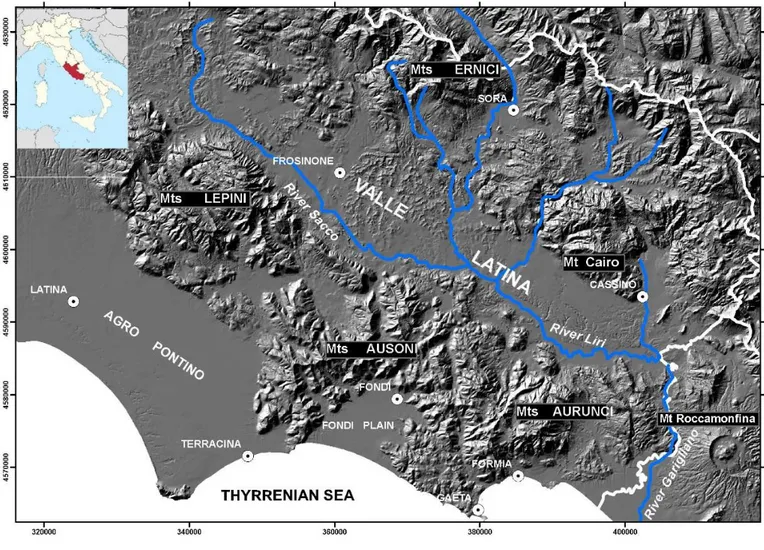
Latium is an administrative region of central Italy with an area of about 17,000 km2, facing the Tyrrhenian Sea. The area considered in the present work is located in the southern portion of the region between N 41° 30' and N 41° 15' latitude and E 12° 30' - E 13° 50' longitude, with an extent of about 4,000 km2 (Fig. 1).

Main landforms in the study area, from the coastline toward the inner land, are: the coastal plains of Agro Pontino, Fondi and the Garigliano river plain; the central calcareous mountain ridge formed by the Lepini, Ausoni and Aurunci mounts (1,500 m above sea level); and the "Valle Latina", a large intermountain basin formed by the Sacco and Liri river valleys, bordered on the north by the Apennine ridge (mounts Ernici, 2000 m, and Monte Cairo massif, 1669 m). All of these landforms show a NW-SE direction, following the main regional tectonic structure.

Main lithologies present in the area are Mesozoic-Paleogene carbonate rocks (central mountain ridge, Monte Cairo), Miocene-Pliocene flysch series (Valle Latina and Garigliano basin) and Pleistocene-Holocene lacustrine, fluviatile and marine-eolian sedimentary deposits (conglomerates, sands and clays in varying successions accumulated in the coastal and intermountain plains).

8

Figure 1. Map of the area

The climate is Csa Mediterranean with mean annual total precipitation around 1,000 mm. However, the Mediterranean character weakens with altitude and landscape variability. The coastal plains show slightly narrower temperature ranges during the year, with mean annual temperatures around 17 °C and low annual rainfall (750-1,000 mm), with respect to the inner zones characterized by colder and more rainy conditions (mean annual temperature around 10 °C and precipitations from 1,250 to 2,000 mm per year).

During the last fifty years prevalent land use has changed from agricultural to industrial through the development of small and medium size industrial settlements spread throughout the territory. This change has been sustained by the abundance of water resources. Farming has shifted toward vegetables, orchards, specialized vineyards, and new cultivations such as kiwi and exotic plants. Animal husbandry is still an important activity in the coastal plains, with quality dairy production from buffalo livestock. Areas over 600 m altitude are covered with forests and shrubs, commonly susceptible to wildfires during summer months. Urban settlements, mainly historical villages of pre-Roman and Medieval origin, are small and dispersed. Main towns are the modern city of Latina (about 120,000 people) founded in 1932 in the Agro Pontino coastal plain, and Frosinone (46,000 people), located in the Valle Latina. Many natural parks and protected areas are present, with a total extent of more than 44,000 hectares.

Soil types in the area can be roughly classified, according to the Soil Regions of Italy, as Cambisols - Leptosols with Luvisols and Fluvisols [12]. Andosols and Regosols are also present in the

9

northwestern and southeastern edges of the area, due to the proximity of main volcanic structures (Vulcano Laziale and Roccamonfina).

An extended description of soils of southern Latium was carried out in the framework of a project of the Faculty of Physical Geography and Soil Science of the University of Amsterdam between 1966 and 1977. The project results were published in a detailed report edited by ENEA (the current Italian National Agency for New Technologies, Energy and Sustainable Economic Development), also including a 1:100,000-scale soil map, with descriptions of soil profiles provided with analytical data [13]. More recently, a soil map of the Sacco river-valley (northwestern part of Valle Latina, 580 km2) was published, derived from a field survey carried out 20 years before aimed at soil classification and land capability evaluation [14]. A soil erodibility assessment was also performed in the same study [15]. Lastly, the earlier Dutch study [13] was integrated and reorganized in order to achieve a systematic soil inventory database covering the entire Province of Latina (2,250 km2) [16].

3. DATA ANALYSIS AND MODEL IMPLEMENTATION

Soil erosion rates can be assessed by means of different techniques and models. The Revised Universal Soil Loss Equation - RUSLE , derived from the former USLE [17], is one of the most widely used empirical models in soil erosion assessment. The reason for its widespread use lies in the RUSLE model's ability to couple simple form with reliable prediction accuracy. The model estimates the long-term yearly rate of soil loss in mass units per unit area (in SI units: Mg ha-1 y-1). Soil loss is obtained as the product of six major factors grouped into two sets representing, respectively, the natural and the human elements acting in soil erosion processes. The first set of factors accounts for: the energy input by rainfall, i.e. the erosive power or erosivity (R factor, MJ mm ha-1 h-1 y-1); the soil erodibility, i.e. the soil susceptibility to erosion per rain erosivity unit (K factor, Mg h MJ-1 mm-1); and the terrain shape expressed by the product of slope length and steepness (LS factor, dimensionless). The other set accounts for the effects of human activity on soil stability and conservation, through the soil cover management and the supporting practice factors (C and P, dimensionless):

) ( )

(R K LS C P

A     (1)

Although the USLE empirical model was initially calibrated for single plots on gentle slopes in agricultural fields, based on long series of observations from about 50 experimental sites in the USA, the worldwide applications that followed its introduction have proved its functionality even in very different environments and areal extents [18-24]. Soil erosion maps at continental and national level using the USLE/RUSLE approach have been drawn in Europe [25]. In Italy, many regional applications can also be cited [26-32]. In these applications, GIS-based (Geographic Information System) spatial processing techniques are employed to convert RUSLE factor point-values (R and K, essentially) into surface polygons. Single maps displaying the areal distribution of R, K, LS, C and P factors are then combined by running the RUSLE model through the specific GIS operator tool to ultimately provide the map of soil erosion rate distribution.

As explained above, rainfall, soil, elevation and land use/cover data are needed to allow application of the RUSLE model. All these data can be obtained from readily available datasets. However, the P factor, related to supporting practices, is generally neglected when dealing with large geographic areas, i.e. regional and national scales, since it is a very local factor whose effects can be significant for plots or small catchment scale assessments.

In the present work the long-term average annual soil erosion rate is estimated, regardless of seasonal and inter-annual variations affecting most of RUSLE factors. Actually, the variables considered in the model equation are subject to variation with time and space. Rain erosivity obviously changes with rainfall throughout the year and from one year to another, due to seasonal and climate variability affecting rainstorm frequency, duration and intensity [33-34]. Soil erodibility changes as a

10

function of soil properties [35,36,37] and climate conditions [38-39]. Nonetheless, intrinsic and time invariant properties such as soil texture and mineralogical composition may be distinguished from dynamic and transient or man-induced properties such as organic matter and water content or surface roughness [40]. Thus, to a first approximation, the K factor could be related to the invariant soil properties only, provided that a sufficiently long period of observation is considered.

Intra- and inter-annual changes are also important, mainly in croplands, with regard to land cover and management factor C as well. Changes are due to management practices, natural growing cycles, or other natural effects affecting plant canopy or health status.

In summary, soil erosion should be estimated at the finest possible detailed time-scale, from monthly to daily or at event-scale, in order to catch the time variability potentially affecting the RUSLE factors. Nevertheless, for the purpose of present work, time variability is here neglected and average yearly reference values for each of the RUSLE factors are estimated and taken into account. Spatial variability and its implications will be discussed.

3.1. Soil erodibility

The K factor was here determined by means of the correlation formula developed by Römkens et al. on the basis of a global soil database [41]. This formula only requires the soil texture as input data:

(2)

where:



_



 fi mi

Dg exp 0.01 ln (3)

Dg represents the geometric mean of soil particle sizes, expressed through the fi percentage of the

corresponding primary grain-size fraction (sand, silt or clay) and the arithmetic mean mi of the extreme

values for that grain-size fraction [42]. In the above-mentioned correlation formula, other soil characteristics such as organic matter content, structure and permeability, as required by the former USLE model and computed by means of the soil erodibility nomograph or its simplified solving equation, are neglected.

The soil textural data utilized here were those published by Sevink et al. [13]. The authors provide a general description of soil types following a subdivision mainly based on landscape and parent material (physiographic units, see Table 1). Each description is accompanied by the detailed characterization of soil profiles, classified according to the FAO/Unesco "Key to Soil Units for the Soil Map of the World" (1974), and their textural and physical-chemical properties. A total of 87 soil profiles and related analytical data were therefore available for use in the present work.

Based on the provided grain-size data related to the topsoil layer, the corresponding K factor was calculated here for each of the 87 described soils by means of the equation (2). In order to proceed with further spatial data processing, the soil profile locations were georeferenced and labeled with the corresponding computed K values in GIS environment.

The spatial distribution of sample points in relation to the overall extent of the considered area was acceptable, apart from a lack of observations in the central calcareous mountain ridge. For this reason, a cursory sampling survey was carried out at the end of 2013 with the aim of filling the gaps in the information available and to provide a more complete database. In this survey, 27 additional topsoil samples were collected in the area of Lepini, Ausoni and Aurunci mountains. Given the extent of the area (about 700 km2), the sampling campaign was mainly planned according to access and logistical economy. This was done by crossing two GIS layers representing the soil map and the road atlas,

                              2 7101 . 0 659 . 1 ) log( 2 1 exp 040 . 0 0034 . 0 Dg K

11

respectively, in order to select a minimum number of representative sampling points easily reachable by vehicle. A complete pedologic profile description of sampled soils was not performed during the field survey, given that only textural data were needed for determining the soil erodibility through the equation (2). Statistical point pattern analysis suggests a satisfying sampling design, since there is no evidence to reject the null hypothesis of spatial random distribution all over the area (2 for Poisson distribution = 0.095; df = 2; p-value = 0.953).

In Table 1, the grain-size compositions and computed K of soil samples are averaged on the basis of the physiographic unit membership, according to [13].

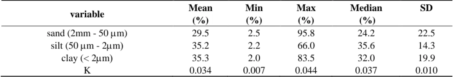
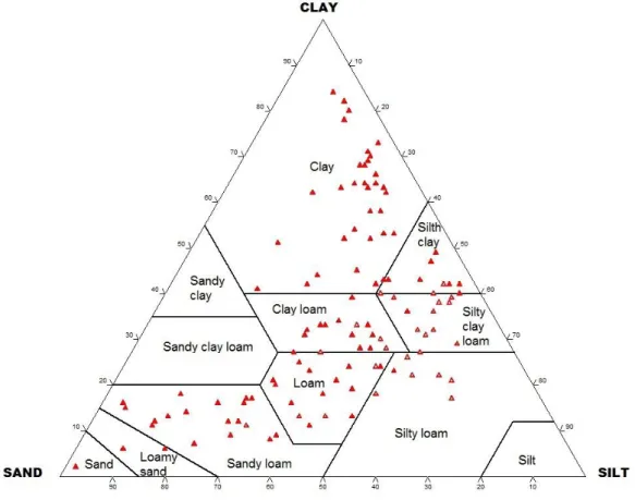
By the USDA classification diagram (Fig. 2) almost half of the analyzed soils (46 %) fall in the clay and sand fields, whereas the remainder (54 %) fall in the fields of variously composed loams. The K-values here obtained outline a soil erodibility from very low to moderate: they vary from a minimum of 0.007 Mg h MJ-1 mm-1 for a sandy soil on a dune deposit at 9 m a.s.l., to a maximum of 0.044 Mg h MJ-1 mm-1 for clay-loam soil types found atop various bedrocks (limestone, shales, lavas, lagoonal clays, lacustrine deposits, meandering stream deposits, alluvial fan deposits, colluvial deposits) at different elevations. Soil samples show an average erodibility of 0.034 Mg h MJ-1 mm-1 and a low dispersion around this value (Table 2).

Table 1. Average textural data and K values in soil samples grouped according to

physiographic units

Physiographic units SAND > 50 m SILT CLAY < 2 m Dg K

Fluvial 25 40 35 0.032 0.038 Colluvial 21 32 47 0.019 0.037 Lacustrine 15 44 41 0.014 0.039 Littoral-eolian 81 8 11 0.390 0.013 Lagoonal 40 22 38 0.109 0.026 Conglomerates 48 30 22 0.082 0.034 Sandstones 57 29 14 0.153 0.025 Shales 29 40 31 0.027 0.044 Limestones 18 43 39 0.024 0.036 Volcanic (Roccamonfina) 38 37 24 0.070 0.036

Volcanic (Vulcano Laziale) 16 23 61 0.007 0.033

Volcanic (Ernici and tuffs of various origin) 33 37 30 0.048 0.037

Table 2. Statistics of soil grain-size fractions and K

variable Mean (%) Min (%) Max (%) Median (%) SD sand (2mm - 50 m) 29.5 2.5 95.8 24.2 22.5 silt (50 m - 2m 35.2 2.2 66.0 35.6 14.3 clay (< 2m 35.3 2.0 83.5 32.0 19.9 K 0.034 0.007 0.044 0.037 0.010

12

Figure 2. USDA soil classification diagram. Filled triangles: soil data from Sevink et al. [13]; open triangles: data from field soil survey (2013)

The K values here obtained are in agreement with those reported in the cited study on the valley of Sacco river [15], where a soil erodibility assessment was performed on the basis of 190 soil profiles by means of three different regression model equations, namely, the EPIC formula [43], the equation also utilized in the present work [41], and the formula proposed by Torri et al. [44]. The authors evidenced that the estimates obtained by the EPIC model, considering the overall samples number comprehensive of all the texture classes, were significantly different and higher than those by the other two methods, whose performances did not deviate too much the one from the other.

In order to derive the erodibility map for the whole area, one method is assigning K values computed for single point locations to the corresponding major soil types represented as area-fields in the available pedological map. However, this point-in-polygon method can lead to biased estimations [37,45], given the spatial variability of soil properties. In recent years, different geostatistical techniques have been introduced in order to predict soil erodibility in non-sampled locations [37,46-49].

In the present work, three different interpolation models have been selected and tested: 1) the Empirical Best Linear Unbiased Predictor based on Residual Maximum Likelihood (REMLEBLUP) -[50]; 2) the Neural Network with refinement [51]; 3) the Kriging with Local Variogram [52-54].

The REML-EBLUP analysis was performed using the SAS/STAT software, version SAS University Edition Software 9.4. Copyright © 2014 SAS Institute Inc. Cary, NC, USA. This technique is a special application of variance component analysis. It is different from the traditional maximum likelihood method as it makes use of a restricted information area in order to search the likelihood function. To the aim of the present work, it can be used as a geostatistical method since the estimated variance components give the parameters to fit the empirical semivariogram. The first part of the analysis, the REML step, aims to detect the model that is least distant from the observed data, i.e. the

13

smallest –2 residual log-likelihood index; while the second part, the EBLUP step, builds the model of spatial covariance that was previously detected, and performs the interpolation at non-observed locations. The strength of REML-EBLUP is in its ability to produce unbiased estimates of the fixed effects, which represent the trend surface, and of the random effects, which capture the local spatial variation. Its validity over other geostatistical methods such as regression kriging has been discussed in the literature [46, 48,55-57].

The Neural Network with refinement model also consists of a two-step procedure. The first step is somewhat similar to regression kriging, but it makes use of neural network analysis (multilayer perception) instead of regression. The second step, identical to regression kriging, is a simple kriging interpolation applied to the derived residuals. The results of the two steps are summed in order to estimate the spatial structure of the statistical variable.

The third model, based on local variogram, is a kriging technique based on a flexible semivariogram model based on the neighborhood structure of each point and it has been implemented by VESPER software [55].

In order to choose the best performing model among the three briefly described just above, testing their stabilities is an essential task . A split sample design has been adopted. A random sample of 80 observations, a subset of the total of 114 K factor values, was arranged in order to build the model, while the remaining 34 observations were used for validation. This procedure tends to avoid overestimation of the goodness of fit and in this respect it appears to function more effectively than others such as the leave-one-out technique. Table 3 presents characteristics of some of the indices commonly employed to deal with this matter. Mean absolute error (MAE), along with mean absolute percentage error (MAPE) and mean squared error (MSE) are measures of total average error. Mean biased error (MBE) takes into account the algebraic residuals instead of the absolute ones (MAE) and it reflects systematic error rather than random error. Furthermore, in order to explore the partition between systematic and random errors, we followed Wilmott's technique of mean squared error (MSE) decomposition in MSEs and MSEu [58,59]. The s and u suffixes stand for the systematic and the stochastic component, respectively. The 95% bootstrap confidence interval of residuals should ideally show a negative sign at the lower limit and a positive sign at the upper limit which indicates a zero centering. Finally, as measure of concordance, the Wilmott D agreement index is displayed. It should ideally approach unity and its strength is its immunity to being affected by outliers. Upon initial inspection of Table 3 no one of single tested methods appears clearly preferable to the others. Model 2 is the only one which satisfies the confidence interval bound limits (from -0.0009 to 0.0035) and it shows a relatively small general error (MAPE = 19%). However, it is not performing in a purely systematic way, as its MBE (0.0013) and MSEs (0.000038) are higher than in model 3 (0.0008 and 0.000032 respectively). Moreover, when transferring this model to descriptive mapping, the visual impact of representation is plagued by excessive spikes and rough edges. In addition, it shows a very high variation coefficient with regard to the other two (Table 3). In short, this model seems precise but inaccurate. From a comparative point of view, Model 1 seems to perform worse than the others, even if the stat indices are generally satisfactory. Finally, model 3 seems preferable to the others because of its systematic error component control (MSEs = 0.000032). It is possibly less precise than Model 2, but is undeniably more accurate. The Willmott D (0.81) supports this interpretation [58,59].

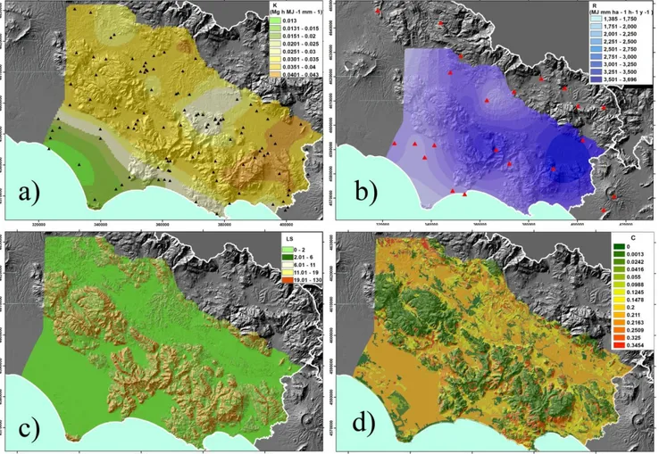
The map obtained by interpolating the K point-values by means of model 3 is shown in Figure 3a. It can be seen that soil erodibility shows a trend related to the main landform traits of the study area. The map depicts a progressive trend from the coastal plains towards the mountainous and inner zones. The highest K values are found on the highest relief portions of the area (Lepini and Ausoni-Aurunci mountains and Mt. Cairo). Lower values in the middle Valle Latina basin correspond to colluvial deposits in karst basins. These results mirror the higher vulnerability of thin soils covering steep rocky hillsides versus mature and deep soils on unconsolidated rocks in flat areas.

14

Table 3. Comparison of goodness of fit indices using validation datasets

Mod. 1

REML-EBLUP

Mod. 2

Neural Network with simple Kriging

refinement Mod. 3 Local variogram Min 0.0130 0.0098 0.0170 Max 0.0430 0.0390 0.0410 Std. dev. 0.0052 0.0100 0.0047 Mean 0.0323 0.0304 0.0322 Variation coeff. 0.1598 0.3289 0.1460 MAE 0.0072 0.0066 0.0076 MAPE 0.2100 0.1900 0.2200 MBE 0.0023 0.0013 0.0008 lower 0.0003 - 0.0009 0.0002 Bootstrap residuals * upper 0.0042 0.0035 0.0041 MSE 0.000068 0.000057 0.000042 MSEs 0.000047 0.000038 0.000032 MSEu 0.000022 0.000019 0.000010 Wilmott's D 0.7000 0.7400 0.8100

* 95% residuals confidence interval, based on 10.000 samples bootstrap analysis

Figure 3. Modeled patterns for RUSLE factors: a) soil erodibility K (black triangles: soil sampling locations); b) rainfall erosivity R (red triangles: rainfall gauging stations); c) topographic factor LS; d) cover management C

15

3.2. Rain erosivity

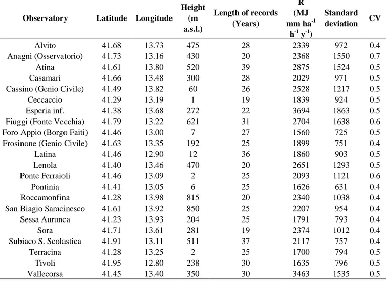
A data-set covering the years since 1950 to 1997 was compiled on the basis of available rainfall data from 20 gauging stations located at different elevations from 1 to 850 m above sea level (Table 4). Data are from the Hydrological Annals published by the former National Hydrographic Service and the current Regional Hydrographic Services of Latium and Campania Regions. For each gauging station the average annual R value has been calculated with reference to the entire observation period:



where N is the number of years with observations and EI30 is the rain erosivity given by the product of

the total kinetic energy E of a single storm (MJ ha-1) and the storm's maximum 30-minute intensity I30

(mm h-1) [17]. The calculation of EI30 requires availability of pluviographs for each single discrete

storm with uniform intensity. To compensate for gaps in such records, annual rainfall erosivity has been calculated by means of the correlation formula by Diodato [60]:

EI_30Rannual12.142





where a, b, and c are, respectively, the total annual rainfall, the annual maximum daily rainfall, and the annual maximum hourly rainfall, all expressed in centimeters. This formula has been proven to be more effective than other correlation models in reproducing the erosive power of rainfall in the Italian peninsular geographic background [60]. The rationale of this formula is that variable a is representative of less erosive rainfall events, with a cumulative effect over long periods, whereas variables b and c describe the very erosive effects of extreme rainfall events such as storms and heavy showers. Moreover, these variables are easily accessible and generally available in long time series.

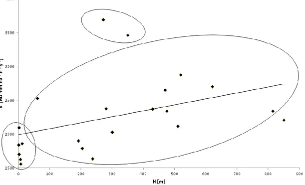
The R factors computed by means of eq. (5) for the 20 gauging stations point out a moderate rain erosivity ranging from a minimum of 1560 to a maximum of 3694 MJ mm ha-1 h-1 y-1 (on average: 2259 MJ mm ha-1 h-1 y-1). In most of the observed cases, erosivity shows a relatively low time-variability around the long-term average in the observed period, as indicated by the standard deviation and coefficient of variation (CV). With regard to the spatial variability, a case-study in the French Alps, where the statistical relationships between heavy rainfall and topography (elevation, exposure and slope steepness) have been investigated, showed that heavy rainfall events measured on short time steps (less than 3 hours) are significantly linked to relief characteristics [61]. As it is defined, the erosivity R applies mainly to heavy rainfall of short duration, therefore, one can expect that R has some relationship with elevation. Nevertheless, no relationship can be identified between R and elevation in southern Latium, basing on available data, as the plot in Fig. 4 clearly shows (r2 = 0.168). Given the low number of observations, attempting a data analysis by more detailed statistical methods is not suitable. However, three subsets may be geographically distinguished within the database, corresponding to the main morphological traits recognized from SW to NE in the investigated area: one groups the rain gauging stations located along the Agro Pontino coastal plain, at an average height of 5 m asl, showing an average R < 2000; the second subset can be identified in the rain gauging stations on the central mountain ridge (average height: 364 m; average R > 3000); the third is given by the rain gauging stations along the Valle Latina (average height: 414 m; average R between 2000 and 3000). The distribution of R values according to this scheme highlights the increase of erosivity from the coastal plain to the first mountain ridge - which can be explained by the barrier effect on wet air masses moving inland from the sea and there discharging the maximum rain energy - and its relative lowering proceeding toward the inter-mountain valley.

16

Table 4. List of rain gauging stations (coordinates in decimal degrees) and average annual

R values with statistics

Observatory Latitude Longitude

Height (m a.s.l.) Length of records (Years) R (MJ mm ha-1 h-1 y-1) Standard deviation CV Alvito 41.68 13.73 475 28 2339 972 0.4 Anagni (Osservatorio) 41.73 13.16 430 20 2368 1550 0.7 Atina 41.61 13.80 520 39 2875 1524 0.5 Casamari 41.66 13.48 300 28 2029 971 0.5

Cassino (Genio Civile) 41.49 13.82 60 26 2528 1217 0.5

Ceccaccio 41.29 13.19 1 19 1839 924 0.5

Esperia inf. 41.38 13.68 272 22 3694 1863 0.5

Fiuggi (Fonte Vecchia) 41.79 13.22 621 31 2704 1638 0.6

Foro Appio (Borgo Faiti) 41.46 13.00 7 27 1560 725 0.5

Frosinone (Genio Civile) 41.63 13.35 192 25 1899 751 0.4

Latina 41.46 12.90 12 36 1860 903 0.5

Lenola 41.40 13.46 470 20 2651 1293 0.5

Ponte Ferraioli 41.46 13.09 2 25 2093 1121 0.6

Pontinia 41.41 13.05 6 25 1626 631 0.4

Roccamonfina 41.28 13.98 815 20 2340 1038 0.4

San Biagio Saracinesco 41.61 13.92 850 25 2207 954 0.4

Sessa Aurunca 41.23 13.93 204 25 1791 793 0.4 Sora 41.71 13.61 281 19 2374 1012 0.4 Subiaco S. Scolastica 41.91 13.11 511 37 2117 757 0.4 Terracina 41.28 13.25 2 25 1700 794 0.5 Tivoli 41.95 12.80 238 30 1635 796 0.5 Vallecorsa 41.45 13.40 350 30 3463 1535 0.5

With regard to rain erosivity mapping, due to the scarcity of observational data, the interpolation of R factors was not performed by a geostatistical method, as it was done in the case of K factor. The use of a minimum curvature spline surface interpolation is clearly preferable in place of other deterministic techniques. Nonetheless, the estimates based on this technique have been validated both in a statistical way and by visual comparison with historical rainfall maps available on the Regional Integrated Agrometeorological Service website, not shown here for copyright reason (http://www.arsial.it/portalearsial/agrometeo/index.asp). About this topic, different interpolation methods, from global (GLS Generalized Least Squares multiple regression) to local (Inverse Distance Weighting IDW and splines) and geostatistical interpolation models (Ordinary Kriging, Universal Kriging and Co-Kriging), have been compared with the aim to map the rainfall erosivity expressed by the R factor and the EI30 index in the Ebro basin (NE Spain) [62]. The study pointed out that all

interpolation methods were able to capture the main spatial pattern of both indices with narrow differences between models under the validation ranking and robustness of predictions. Local interpolation methods yielded the best results but the resulting maps were affected by excessive weights given to local observations.

17

Figure 4. Plot of the relationship between R factor and altitude. In the circles, subsets of rainfall observatories cited in the text

Table 5 shows the results of leave-one-out validation. The indices reported in this table are encouraging, although this kind of validation is generally considered too optimistic. Above all, the Willmott’s D is close to maximum agreement, whereas mean absolute percentage error (MAPE) is just 6%. The 95% bootstrap confidence interval contains the zero value and the systematic error source is undersized (6530, which is only 20% of the total estimated error) .

Table 5. Leave-one-out validation of R factor interpolation by means of minimum

curvature spline

Minimum curvature spline

MAE 138.2 MAPE 6% MBE -64 lower -147.7 Bootstrap residuals* upper 10.4 MSE 39763 MSEs 6530 MSEu 33234 Wilmott's D 0.96

18

The rain erosivity map obtained by the interpolation of single-point R values is shown in Figure 3b where blue-colored bands of iso-erosivity are modeled by taking into account the entire listed rainfall dataset (Table 4) comprehensive of some rain gauging stations located outside of the investigated area. The map depicts the presence of a split nucleus of high erosivity, located on the central mountain ridge and centered on the rain gauging stations where heaviest rainfall has been recorded, surrounded by lower erosivity belts corresponding to the coastal plains and the interior valleys.

3.3. Slope length and steepness

The LS topographic factor was computed on the basis of a 20 m resolution DEM, using a public processing code [63,64] running algorithms based on raster grid cumulation and maximum downhill slope angle methods. The executable program for LS calculation is downloadable at the link: http://www.iamg.org/documents/oldftp/VOL30/v30-09-11.zip. In this way, differently from the previous factors, the LS factor was directly computed for each of the 20 m cells of the DEM grid covering the whole area.

The resulting map shows that LS values are generally very low (mean: 5.57), but with high variability (SD = 8.81), the lowest values being obviously localized on the flat portions of the area and the highest ones on the hillsides. LS values less than 2 cover 58% of the whole area, while the extreme values (>19) affect 9% only (Fig. 3c).

3.4. Land cover management

Factor C is rather complex to evaluate. Many sub-factors must be estimated, according to the RUSLE handbook [8], in order to parameterize the effect of actual land cover on soil erosion. Such sub-factors are: previous land-use, canopy-cover, surface cover, surface roughness, and soil moisture. Moreover, these sub-factors should be estimated for each time period of the year over which the single sub-factors can be assumed to remain constant, considering the seasonal variations due to crop rotation or other natural effects (climate, plant health conditions etc.). Thus, adopting average values for the various land cover categories that can be recognized over a given area is a rough approximation. However, the scale of investigation of the present work does not allow to make more accurate estimates. Therefore, very general C values were here adopted in order to roughly quantify the effect of land cover management on soil erosion due to natural agents.

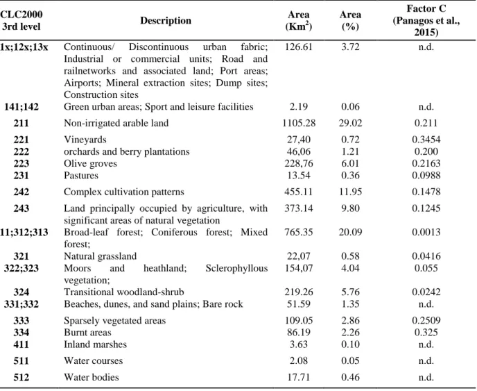
The C factor was attributed on the basis of the 3rd level classification of the Corine - Land Cover 2000 map of Latium. Due to the unavailability of observed data for the study area, the C values assigned to the CLC classes here recognized are those provided by the European Soil Data Centre at the European scale [65]. The correspondence between land cover classes and C factor is shown in Table 6. As shown in the table and in Figure 3d, the most represented land cover class in the investigated area is given by arables and cultivations (~ 60 %) whose C values are varying from 0.1245 to 0.3454, whereas forested and scrub or herbaceous vegetated areas, having a C factor from 0.0013 to 0.055, are 30% of the area. All things considered, the map of C factor was here drawn by means of a point-in-polygon method, differently from the grid-based method used for the other RUSLE factors maps.

An alternative method for deriving and mapping the C factor in a distributed way (at grid-cell level) is utilizing the Normalized Difference Vegetation Index (NDVI), helpful to quickly identify vegetated and non-vegetated areas from airborne or satellite imageries. The NDVI is an indicator of plant reflectance in the red and near-infrared spectral region and varies between -1 and 1, where negative and very low positive values (up to 0.1 - 0.2) are typically characteristic of water bodies, snow, bare soil and built-up areas, whereas vegetated areas have NDVI values larger than 0.1. A linear correlation between the C factor and the NDVI was found by De Jong [66]:

NDVI

19

Table 6. CLC2000 classes mapped in the area and assigned C values

CLC2000 3rd level Description Area (Km2) Area (%) Factor C (Panagos et al., 2015) 11x;12x;13x Continuous/ Discontinuous urban fabric;

Industrial or commercial units; Road and railnetworks and associated land; Port areas; Airports; Mineral extraction sites; Dump sites; Construction sites

126.61 3.72 n.d.

141;142 Green urban areas; Sport and leisure facilities 2.19 0.06 n.d.

211 Non-irrigated arable land 1105.28 29.02 0.211

221 222 223

Vineyards

orchards and berry plantations Olive groves 27,40 46,06 228,76 0.72 1.21 6.01 0.3454 0.200 0.2163 231 Pastures 13.54 0.36 0.0988

242 Complex cultivation patterns 455.11 11.95 0.1478 243 Land principally occupied by agriculture, with

significant areas of natural vegetation

373.14 9.80 0.1245

311;312;313 Broad-leaf forest; Coniferous forest; Mixed forest; 765.35 20.09 0.0013 321 322;323 324 Natural grassland

Moors and heathland; Sclerophyllous vegetation; Transitional woodland-shrub 22,07 154,07 219.26 0.58 4.04 5.76 0.0416 0.055 0.0242 331;332 Beaches, dunes, and sand plains; Bare rock 51.59 1.35 n.d.

333 334

Sparsely vegetated areas Burnt areas 109.05 86.19 2.86 2.26 0.2509 0.325 411 Inland marshes 3.63 0.10 n.d. 511 Water courses 2.08 0.05 n.d. 512 Water bodies 17.71 0.46 n.d.

However, this relation was characterized by a weak coefficient (r = - 0.64). In order to improve this relation, an exponential equation was thereafter suggested by Van der Knijff et al. [67]:

        NDVI NDVI C 1 2 exp (7)

This equation has been used in different studies worldwide since its publication, although the authors themselves acknowledged the lack of field evidence to justify the use of their equation. Moreover, equation (7) was obtained on the basis of a low-resolution satellite platform (NOAA-AVHRR, 1-km pixel size) that makes up-scaling unreliable.

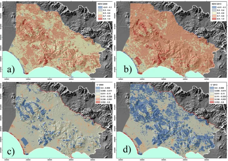
As an attempt to test the validity of the method, available time-series of average annual NDVI from MODIS images (250 m resolution) covering the years from 2000 to 2013 was here utilized with the aim of deriving the land management factor by means of equation (7). The analysis was limited to the extremes of the period under consideration, thus, two maps of NDVI pattern were drawn for years 2000 and 2013 (Fig. 5a-b). Incidentally, the comparison between the two maps highlights a greening trend of natural vegetation areas, in agreement with vegetation studies in other parts of Italy [68]. This trend is probably linked to the temperature and precipitation changes that have occurred since the year 2000 in central-southern Italy [69]. The difference between the two vegetation indices is also reflected in the corresponding land management factor (C') maps. On the other hand, as can be seen in figures 5c-d, the application of equation (7) produced C' values quite different from those provided by the

20

ESDC and adopted here. In fact, the NDVI-derived factors show a wider range (from 0 to 0.8 ) than the CLC2000-based factors reported in Table 6. Moreover, within the same land-cover category, differences can be up to one or two orders of magnitude. Differently from what was pointed out by Van der Knijff et al. [67] about unrealistically high land cover factor produced by equation (7), especially for woodland and grassland, the MODIS-based NDVI-derived C' factor here obtained appears to be consistent with generally accepted values for woodlands. Some correspondence between C and C' maps can be recognized on forested areas. On the contrary, no match can be found on other categories such as non-irrigated arable land and complex cultivation patterns or vineyards, orchards, and olive groves actually showing NDVI-derived C' values generally lower than 0.1.

Similar inconsistencies were proved in the framework of a research project recently carried out in Thailand [70]. This study compared the results obtained by applying the prediction models cited above [66,67], and a specific model calibrated on local fieldwork data, revealing wide differences in magnitude and relative spatial pattern of derived C values.

These uncertain results suggest that it is advisable, in the present phase, to avoid utilizing the NDVI-based methodology in the studied area and to await further investigation for a more critical analysis.

21

4. RESULTS AND DISCUSSION

Combining the layers related to the different RUSLE factors in GIS environment, according to the model equation (1), the soil loss map of southern Latium is obtained. One can distinguish between the

potential soil loss, only due to the natural components of the model (K, R and LS layers) and the actual soil loss by introducing the C factor taking into account the effect of land cover management on

natural erosion.

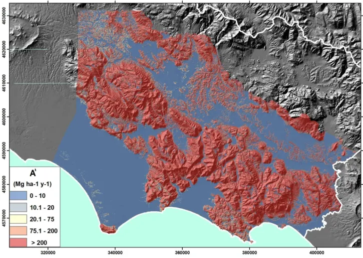
The map of the average yearly potential soil loss (A') (Fig. 6a) shows a sharp difference in potential soil loss rate between flat areas and steep mountain zones. This evidence would suggest that the landscape relief, quantified by the LS factor, strongly affects the erosion potential more than either rain erosivity or inherent soil erodibility.

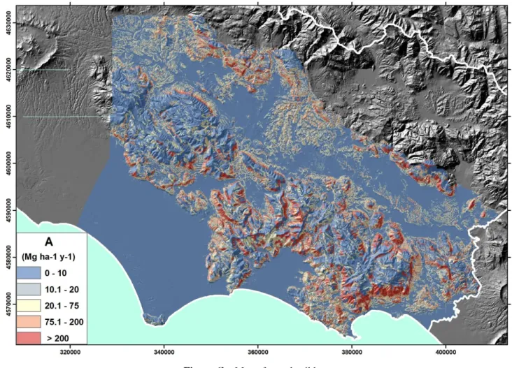
The effect of the C factor on calculation produced different soil erosion amounts and patterns (A) in comparison with the potential soil loss estimate, pointing out the key-role played by land cover management (Fig. 6b). The resulting actual soil loss map shows that most of the area is characterized by very low or negligible soil erosion rates (< 10 Mg ha-1 year -1). Coastal plains and intermountain valleys, as expected, but also hilly gently-sloping areas are comprised in this erosion class. Major soil loss affects many areas on the central mountain ridge and the reliefs bordering the Valle Latina. Extreme values ( > 200 Mg ha-1 year -1) are prevalent in these sectors. The average soil loss rate referred to the overall area is about 44 Mg ha-1 year -1. As explained before, in the present work, the C factor was not derived from field observations but from general data available in the literature. For this reason, the impact of this factor on estimated soil erosion rates in the investigated area can be considered merely approximate.

22

Figure 6b. Map of actual soil loss

In order to validate the erosion rates here supplied, a comparison between observed and predicted data could be helpful. Unfortunately, direct measurements are not available. Moreover, given the extension of the area here investigated (about 4,000 km2), observations should be carried out in several points scattered throughout the area. Furthermore, the same observations should be referred to a long time-span, enough to obtain a significant average soil loss rate. The only observations available in Latium have been carried out for few years in the past, on a few plots located in the country around the city of Rome, outside of the studied area [71,72,73].

A comparison may be attempted with the map previously produced by the European Soil Bureau [11] at the national scale, cited in the introduction, both from a trend and a class-by-class point of view, notwithstanding the differences in data sources and scale resolution. From the first point of view, the erosion rate assessed in southern Latium in the present work appears overestimated of about 30 ha-1 year -1, on average, compared to the map by ESB in the same area. Nevertheless, the statistical correlation between the two raster maps, on a cell resolution of 250 m, points out a good agreement in soil loss pattern (Spearman's rank correlation coefficient  = 0.58). To visualize the differences on a statistical basis, a map of p-values (significance level) for the algebraic differences, has been drawn by means of a simulation technique based on 9,999 permutation. This map, shown in Figure 7, points out the areas showing p-values ≤ 0.05 and marked in red and ochre colors where differences, whether positive or negative, are statistically significant. As can be seen, a good consistency between the two maps can be recognized, since the cells marked by non-significant difference are the largest majority. More critical appears the consistency between the two maps from a class-by-class point of view as can be seen from Table 7 showing the sharing percentage of cells for each erosion class. In general, the diagonal cells express the full classification agreement, while the off-diagonal cells point out different seriousness of disagreement according to their distance from the ideal diagonal cells. Actually, while a

23

good similarity is held in the lowest class (more than 80% of the cells assigned to the class 0-10 Mg ha-1 year -1 in our map falls in the homologue class in the ESB map), the agreement worsens moving toward the highest class (> 200 Mg ha-1 year -1) where just 0.2% of the cells of our map is consistent with the ESB estimate, the majority being included in lower classes.

Table 7. Agreement between southern Latium and ESB map by cells distribution in

erosion classes

Southern Latium (present work)

ESB 2003 0 - 10 10 - 20 20 - 75 75 - 200 > 200 Totale 0 - 10 81.4 54.6 42.1 27.5 13.0 66.2 10 - 20 7.7 19.3 18.2 19.9 9.0 10.9 20 - 75 9.3 22.1 32.8 42.1 51.8 18.4 75 - 200 1.6 4.0 6.8 10.3 26.0 4.6 > 200 0.0 0.0 0.0 0.1 0.2 0.0 Totale 100 100 100 100 100 100

Figure 7 Map of significance level (p-values) for the difference between the ESB and the present work model estimates.

24

This circumstance can be interpreted as due to a scale-factor whose effect is amplified with growing estimated erosion but not to such an extent to invalidate the general trend. Given the lower spatial resolution of the ESB map (250 m) compared with the 20 m resolution here utilized, it is likely that the topographic factor LS could affect the result. Further investigations will allow us to better understand the role played by the LS factor in determining the final result at different geographic scales.

After all these considerations, when validation data are unavailable, theoretical assessments can just give an idea of the potential and impact of erosion processes. Anyway, they can help to address suitable land policies. So, the map of soil loss here obtained can provide a useful snapshot of soil erosion potential in southern Latium. Moreover, it can be reclassified in terms of soil erosion severity in order to represent different degrees of risk and provide a more usable tool for policy makers. To this aim, no standards are yet established in the scientific literature.

The concept of soil loss tolerance is widely accepted, implying a maximum threshold established at 10~13 Mg ha-1 year-1 [17,74], but this limit can be lower in the case of shallow soils or slower pedogenesis processes, as occur in the Mediterranean environment [75, 28]. The cited limit can help to univocally define the lower ranges of soil erosion (very slight to slight), but no criteria are commonly recognized to establish the number and the intervals for the other ranges. Different classifications and techniques have been suggested and employed in recent literature [21, 23, 24, 28, 29], often without justification for the adopted class intervals. To avoid the introduction of subjectivity in soil erosion classification and allow the comparison in small-scale erosion risk maps, the fuzzy mathematics and class membership has been suggested as supporting techniques [44,76,77]. More specifically, a classification system more oriented towards policymakers in designing conservation programs for croplands was proposed [78]. The erosion potential is categorized into four classes, from non-erosive to highly erosive with two intermediate classes, avoiding arbitrary and qualitative designation of erosiveness. After separating the physical (RKLS) and management (CP) components of the RUSLE, the hinge-numbers of the proposed scheme are the following: the value of the tolerable soil loss rate (T) - established by the U.S.D.A. at 11 Mg ha-1 year-1 (5 ton acre-1 in U.S. Customary Units) for cropland; the maximum CP recorded in the U.S. National Resources Inventory of 1977 (0.7); and the minimum CP for intensive row crop agriculture (set equal to 0.1). From these numbers, the lower and the upper bounds for RKLS were obtained to define the classes of erosion [78].

The classification described above is specifically agronomic and management-oriented and is based on available CP data records. An alternative system was proposed by Zachar for the classification of soil removal processes based on six-level intensities [79]. According to this classification, originally expressed in volumetric units, the soil loss estimates in southern Latium can be summarized as shown in Table 8 where erosion classes are expressed in mass of soil loss by considering an average soil bulk-density of 1.2 g/cm³.

Table 8. Erosion classes and areal distribution

Erosion class Soil loss

(Mg ha-1 y-1)

Area Km2

Area %

Nil or negligible erosion 0.0–0.6 1968 52.2

Slight erosion 0.6–6 493 13.1

Moderate erosion 6.0–18 241 6.4

Severe erosion 18–60 476 12.6

Very severe erosion 60–240 414 11.0

25

5. CONCLUSIONS

The soil erosion map of southern Latium has been drawn thanks to the suitability of the RUSLE model for applications at small-medium scale using few available data. The RUSLE model was run in GIS environment by combining different maps (or layers), each representing one of the model's factors. Limits and uncertainties in interpolating and mapping the RUSLE factors have been discussed. The main question in using RUSLE as well as other models at small (i.e. regional or sub-regional) scale, concerns the extrapolation of quantities, e.g. soil erodibility and rainfall erosivity measured at single points, to surrounding space. Another question is the assessment of uncertainty in the estimates. To this aim, the robustness and reliability of algorithms and correlation models utilized in the present study for calculation of K and R factors have already been discussed by others here cited. Moreover, the employment of statistical tools, as performed in the present work, is helpful in testing the reliability and in assessing the spatial uncertainty of estimates in the study area.

In summary, the soil erodibility map of southern Latium was obtained by interpolating 114 sampling points, where the K factor was calculated on the basis of soil textural data, using Kriging with Local Variogram. This latter proved to be better than other techniques such as the REML-EBLUP and the Neural Network with refinement. The map shows a progressive trend in K values distribution from the coastal plains towards the mountainous and inner zones, reflecting the higher vulnerability of thin soils covering steep rocky hillsides versus mature and deep soils on unconsolidated rock in flat areas.

The rain erosivity map was drawn by interpolating R factor values calculated on the basis of rainfall data records in 20 gauging stations located at different elevations. It shows the presence of a split nucleus of major erosivity, located on the central mountain ridge, surrounded by lower erosivity belts corresponding to the coastal plains and the interior valleys.

The slope length and steepness map (LS factor) was compiled on the basis of a 20 m resolution DEM by applying an automatic computational procedure at each cell of the DEM. The resulting map shows that, on average, the area is characterized by low LS values but with high variability, the lowest values being obviously on the flat portions and the highest ones on the hillsides.

The land cover and management map (C factor) was drawn by means of a point-in-polygon method on the basis of the 3rd level classification of the Corine Land Cover 2000 map of Latium. The C factor values here employed were not derived from field observations but from general data available in the literature. By the way, the areal extent requires utilizing a simplified method different from the RUSLE handbook procedure. To this aim, it is controversial which methodology is more appropriate for assigning C factors in small scale applications of RUSLE. Even though simplified annual values are available in the literature for main cultivation types, they are commonly inconsistent between different authors. The methodology to derive the land cover factor from remote Earth observation appears promising, but the attempt made in the present study showed the need to develop a correlation model more robust than those proposed in the literature so far, based on NDVI (or other vegetation indices) from high-resolution imageries. Furthermore, analysis of NDVI changes in the 2000-2013 data series for southern Latium encourages additional investigations on both rainfall and NDVI patterns on multi-temporal scale.

The soil erosion map obtained by combining the different RUSLE factor maps shows that most of the area is characterized by very low or negligible soil erosion rates, on average. Major soil loss affects areas on the central mountain ridge and inland areas with major relief. In order to provide a more useful map for policy makers, a classification criterion emphasizing soil erosion severity has been utilized.

Notwithstanding the lack of observation data in support of the modeled soil loss rates, the work here presented has the worth to demonstrate that the problem of erosion can have relevant effects on the investigated area. This item seems to be not perceived by decision makers, so, the present work points out the need to address field activities and further investigations to better understand the erosion processes underway.

26

Acknowledgments

Thanks to Todd Hinkley (Scientist Emeritus - U.S. Geological Survey) for checking the English writing.

REFERENCES

1. Crutzen, P.J. Benvenuti nell'Antropocene. L'uomo ha cambiato il clima, la Terra entra in una nuova era. Editore Mondadori , Milano, 2005, 94 pp.

2. Ferrara, V.; Farruggia, A. Clima: istruzioni per l’uso. I fenomeni, gli effetti, le strategie. Edizioni Ambiente, Milano, 2007.

3. Rusco, E.; Montanarella, L.; Tiberi, M.; Rossini, L.; Ricci, P.; Ciabocco, G.; Budini, A.; Bernacconi, C. Implementazione a livello regionale della proposta di direttiva quadro sui suoli in

Europa. European Commission - Joint Research Centre 2007, EUR 22953 IT, ISSN 1018-5593,

65 pp.

4. IPCC - Intergovernmental Panel on Climate Change Climate change 2013 - The physical science

basis Summary for policymakers. Working Group I, Contribution to the Fifth Assessment Report

of the Intergovernmental Panel on Climate Change, WMO - UNEP, 2013 .

5. Paolanti, M. I suoli del Lazio: caratteristiche, minacce e sistemi di conservazione. Venerdì culturali FIDAF, SIGEA, ARDAF Ordine dei Dottori Agronomi e dei Dottori Forestali di Roma 7 Dicembre 2012

6. Napoli, R. and Rivieccio, R. Sviluppo, applicazione e validazione di metodi di rilevamento e rappresentazione cartografica per la realizzazione della Carta dei suoli della Regione Latium a scala 1:250.000. Seminario CRA RPS - ARSIAL, Roma 10 Maggio 2013 http://rps.entecra.it/research.htm

7. Renard, K.G.; Foster, G.R.; Weesies, G.A.; Porter, P.. RUSLE-revised universal soil loss equation. Journal of Soil and Water Conservation 1991 , 46, 30-33 .

8. Renard, K.G.; Foster, G.R.; Weesies, G.A.; McCool, D.K.; Yoder, D.C. Predicting soil erosion by

water - a guide to conservation planning with the revised universal soil loss equation (RUSLE).

United States Department of Agriculture, Agricultural Research Service (USDA-ARS) Handbook n° 703, 1996, United States Government Printing Office, Washington, DC .

9. Zini, A.; Grauso, S.; Verrubbi, V.; Falconi, L.; Leoni, G.; Puglisi, C. The RUSLE erosion index as a proxy indicator for debris flow susceptibility. Landslides 2014, online first DOI 10.1007/s10346-014-0515-8.

10. Van der Knijff JM, Jones RJA & Montanarella L Soil erosion risk assessment in Italy. European Soil Bureau - JRC, EUR 19022 EN, 1999, 50pp

11. Grimm, M.; Jones, R.J.A.; Rusco, E. and Montanarella, L. Soil Erosion Risk in Italy: a revised USLE approach. European Soil Bureau Research Report No 11, 2003, EUR 20677 EN.

12. Costantini, E.; Urbano, F.; L’Abate, G. (2012) Soil Regions of Italy. Available online: www.soilmaps.it

13. Sevink, J.; Remmelzwaal, A.; Spaargaren, O.C. The soils of southern Latium and adjacent Campania. ENEA 1984, RT/PAS/84/10, 142 pp.