Classification models and algorithms in application of multi-sensor systems to detection and identification of gases

(1)

Classification Models and Algorithms in

Application of Multi–Sensor Systems to

Detection and Identification of Gases

Walaa Khalaf

(2)

(3)

To my family, and

the woman who gave me

the patience and the courage

(4)

(5)

Acknowledgement

It seems that the long way is coming to its end and it is time to say ”Thanks” to all of you who walked along with me and shared ”the good and the bad”. I thank you a lot my dearest friend professor Alfredo Eisenberg, for all the assistance that you offered me to finish my study and my dream to get the Ph.D. degree, also to my great supervisor pro-fessor Manlio Gaudioso, really I do not have enough words to appreciate what they offered me, but I am sure they know my feelings toward them. I would like to present my thanks to my brother Dr. Falah Alwaely, without him I could not get this chance to study here, also to my wife Noor Hashim, for all her support. Big kiss to my dear friend Mohammed Issa and I am thanking him for not complaining about many destroyed weekends, helping me in translations and grammar corrections.

Coming to the ”professional” part, that was much more than just pro-fessional, one big ”Thank” to professor Giuseppe Cocorullo and professor Calogero Pace, whom I learned a lot from them. ”Regards and thanks” to everybody at the Department of D.E.I.S. (Dipartimento di Elettron-ica, Informatica e Sistemistica)–University of Calabria, especially my col-leagues Giuseppe Fedele, Annabella Astorino, Enrico Gorgone, Antonio Fuduli, Marcello Sammarra, Luigi Moccia, Giovanni Giallombardo, Gre-gorio Sorrentino, Flavia Monaco, Giuseppina Bonavita, and Giovanna Miglionico. Finally, I should thank the people who accommodated me here, at the University of Calabria, and made me feel at home.

(6)

(7)

Abstract

The objective of the thesis is to adopt advanced machine learning tech-niques in the analysis of the output of sensor systems. In particular we have focused on the SVM (Support Vector Machine) approach to classi-fication and regression, and we have tailored such approach for the area of sensor systems of the ”electronic nose” type.

We designed an Electronic Nose (ENose), containing 8 sensors, 5 of them being gas sensors, and the other 3 being a Temperature, a Humidity, and a Pressure sensor, respectively. Our system (Electronic Nose) has the ability to identify the type of gas, and then to estimate its concentration. To identify the type of gas we used as classification and regression technique the so called Support Vector Machine (SVM) approach, which is based on statistical learning theory and has been proposed in the broad learning field. The Kernel methods are applied in the context of SVM, to improve the classification quality. Classification means finding the best divider (separator) between two or more different classes without or with minimum number of errors. Many methods for pattern recognition or classification are based on neural network or other complex mathematical models.

In this thesis we describe the hardware equipment which has been designed and implemented. We survey the SVM approach for machine learning and report on our experimentation.

(8)

(9)

List of Tables

4.1 Gas concentration vs. gas volume . . . 63

4.2 Methanol concentration vs. methanol quantity . . . 64

4.3 Concentrations vs. Ethanol, Acetone, and Benzene quan-tities . . . 65

4.4 Multiple C values vs. classification rate with linear kernel 78

4.5 Multiple C values vs. classification rate for different values of sigma with 3rd degree polynomial kernel . . . 79

4.6 Multiple C values vs. classification rate for different values of σ with RBF kernel . . . . 79

4.7 Multiple C values in the case of linear kernel . . . . 80

4.8 Multiple C and σ values with polynomial kernel of 3rd degree . . . 81

4.9 Multiple C and σ values with RBF kernel . . . . 81

(12)

(13)

List of Figures

1.1 An input–output function . . . 3

1.2 Different Shapes and Sizes of Clusters . . . 7

2.1 VC–Dimension Illustration . . . 16

2.2 Structure of a nested Hypothesis spaces . . . 19

2.3 Separating hyperplanes in a two–dimensional space. An optimal hyperplane with a maximum margin. The dashed lines are not optimal hyperplanes . . . 20

2.4 Optimal separating hyperplane in a two–dimensional space and the distance between it and any sample . . . 22

2.5 Constraining the Canonical Hyperplanes . . . 24

2.6 The optimal hyperplane is orthogonal to the shortest line connecting the convex hulls of the two classes (dotted) . 25 2.7 Nonseparable case, slack variables are defined that corre-spond to the deviation from the margin borders. . . 29

2.8 A feature map can simplify the classification task. . . 33

2.9 Mapping the input space into a high dimensional feature space. . . 36

2.10 The insensitive band for a one dimensional linear regres-sion problem . . . 39

2.11 The insensitive band for a one dimensional non–linear re-gression problem . . . 39

4.1 Block diagram of the system . . . 62

4.2 Sensitivity characteristic for the sensor type TGS 813 . . 66

4.3 Sensitivity characteristic for the sensor type TGS 822 . . 68

(14)

4.6 Temperature vs. Temperature Error Multiplier . . . 72

4.7 First two principal components for the experimental data set . . . 75

(15)

List of Symbols

n Number of samples

d Number of input variables

Rd _{Euclidean Space d-dimensional}

G Finite set of classes

Ω Set of parameters, as in w ∈ Ω

F (x) Cumulative probability distribution function (cdf)

p(x) Probability density function (pdf)

L Loss function

P (x, y) Joint probability density function p(x|y) Conditional density

R Risk function

Λ Set of abstract parameters

H Hypothesis space h VC–dimension k.k Norm γ Margin d Signed distance F Feature space α Lagrange multipliers L Primal Lagrangian W Dual Lagrangian IX

(16)

hx.zi Inner (dot) product between x and z

φ : X → F Mapping to feature space K(x, z) Kernel hφ(x).φ(z)i

ppm Parts per million

cc Cubic centimeter

MW Molecular weight of gas in gram/mol

ρ Liquid density in gram/cm3

d Gas density in gram/liter

(17)

Introduction

We present an Electronic Nose (ENose) which is aimed both at identifying the type of gas and at estimating its concentration. Our system contains 8 sensors, 5 of them being gas sensors, whose sensing element is a tin dioxide (SnO2) semiconductor, the remaining being a temperature sensor,

a humidity sensor, and a pressure sensor. Our integrated hardware-software system uses some machine learning principles to identify at first a new gas sample, and then to estimate its concentration.

In particular we adopt a training model using the Support Vector Machine (SVM) approach to teach the system how to discriminate among different gases, this mean working as classifier, then we apply another training model using also the SVM approach, but here working as an estimator, for each type of gas, to predict its concentration.

We deal with the problems of gases detection and recognition as well as with the estimation of their concentrations. In fact, detection and recognition can be seen as a two–class and a multi–class classifica-tion problem, respectively. The detecclassifica-tion of volatile organic compounds (VOCs) has become a serious task in many fields, because the fast evapo-ration rate and toxic nature of VOCs could be dangerous at high concen-tration levels in air and working ambient for the health of human beings. In fact, the VOCs are also considered as the main reason for allergic pathologies, skin and lung diseases.

To identify the type of gas we use the support vector machine (SVM) approach which was introduced by Vapnik as a classification tool. The SVM method strongly relies on statistical learning theory. Classification is based on the idea of finding the best separating hyperplane (in terms of classification error and separation margin) of two point–sets in the

(18)

Kernel transformations within the SVM context.

We adopt a multi–sensor scheme and useful information is gathered by combining the outputs of the different sensors. The use of just one sensor does not allow in general to identify the gas. In fact the same sensor output may correspond to different concentrations of many dif-ferent gases. On the other hand by combining the information coming from several sensors of diverse types we identify the gas and estimate its concentration. We will present the description of our system, producing the details of its construction.

The results of our experiments on four different types of gases (Methanol, Ethanol, Acetone, and Benzene) have been particularly encouraging both in terms of classification errors and concentration prediction.

(19)

1

Chapter 1 Machine Learning and

Classification

This chapter introduces the principles and importance of learning method-ology which is the approach of using examples to synthesize knowledge. The learning problems can be subdivided into four classes:

• Density Estimation: Let f be an unknown density function in Rd_,

and X1, . . . , XN a random sample with distribution f : provide an

estimator ˆfN based on the data.

• Clustering: The process of organizing objects into groups whose members are similar. A cluster is therefore a collection of objects which are similar between themselves and are dissimilar to the ob-jects belonging to the other clusters.

• Classification: Given a training set (x1, y1), . . . , (xN, yN),

consid-ered as a sample of pairs of random variables (X, Y ) with xk ∈ Rd

and ykin a finite set G of classes, find a function ˆfn: Rd→ G which

is the best prediction of the true class.

• Regression: Given a training set (x1, y1), . . . , (xN, yN), considered

as a sample of pairs of random variables (X, Y ) with xk ∈ Rd and

yk∈ Rq, find a function ˆfn : Rd → Rq to approximate E(Y |X).

(20)

We can easily understand the importance of machine learning in many computer–based real world applications. In the sequel we give a survey of the above mentioned classes of problems.

1.1 Machine Learning

Learning is the process of estimating an unknown function or structure of a system using a limited number of observations. There are two major settings of learning, the first one called supervised learning which is deriv-ing the required output from a set of inputs. Curve–fittderiv-ing is a simple ex-ample of supervised learning of a function, the exex-amples of input/output functionality are referred to as the training data [18, 25, 35]. The sec-ond type is called unsupervised learning, which is the case when having a training set of vectors without function (output) values for them, the learning task is to gain some understanding of the process that generated the data. This type of learning includes density estimation, clustering, learning the support of a distribution, and so on [8, 14, 18].

There are several ways in which the training set can be used to pro-duce a hypothesis function. The batch learning when the training set is available and used all at once to compute the hypothesis function. The entire training set is possibly used to modify a current hypothesis iter-atively until an acceptable hypothesis is obtained. The online learning uses only one example at a time, and updates the current hypothesis depending on the response to each new example [11].

The learning problem is divided into two parts: specification and esti-mation. Specification consists in determining the parametric form of the unknown distributions, while estimation is the process of determining parameters that characterize the specified distributions. The two induc-tive principles that are most commonly used in the learning process are the Empirical Risk Minimization (ERM) and the Maximum Likelihood (ML).

Machine learning is not just a data base management problem; it is also a part of artificial intelligence. To be intelligent, a system that is in a changing environment should have the ability to learn. If the

(21)

1.1. Machine Learning 3

system can learn and adapt to such changes, the system designer need not predict and provide solutions for all possible situations. Machine learning requires design of computer programs to optimize a performance criterion using example data or past experience. We have a model defined up to some parameters, and learning is the execution of a computer program to optimize such parameters using the training data or past experience. The model may be predictive to make predictions in the future, or descriptive to gain knowledge from data, or both. Machine learning also helps us to find solutions to many problems in vision, speech recognition, and robotics [35].

1.1.1 Input and Output Functions

The situation sketched in Figure 1.1, is when there exists a function

f , and the learner job is to guess what it is. We denote by h the

hypothesis of the function to be learned. Both f and h are functions of a vector–valued input X = (x1, x2, . . . , xi, . . . , xd) which has d components.

Function h is being implemented by a device that has X as input and

h(X) as output. Both f and h themselves may be vector–valued.

xi x1 xd Training Set: Ξ = X1, X2, . . . Xi, . . . , Xm X = h ∈ H h(X) h

(22)

We assume a priori that the hypothesized function h is selected from a class of functions H. Sometimes we know that f also belongs to this class or to a subset of this class. We select h based on a training set, Ξ, of m input vector examples.

The input vector is called by a variety of names, some of these are

in-put vector, pattern vector, feature vector, sample, example, and instance.

The components, xi, of the input vector are variously called features,

attributes, input variables, and components. The output may be a real

number, in which case the process embodying the function, h, is called a

function estimator, and the output is called an output value or estimate.

Alternatively, the output may be a categorical value, in which case the process embodying h is variously called a classifier,a recognizer, or a

cat-egorizer, and the output itself is called a label, a class, a category, or a decision.

1.2 Density Estimation

A classical unsupervised learning task is density estimation. We assume that f (x, w), w ∈ Ω is a set of densities where w is an M-dimensional vector. Let us assume that the unknown density f (x, w0) belongs to this

class. Assuming that the unlabeled observations (training data)

X = [x1, . . . , xn] were generated independently and identically distributed

(i.i.d.) according to some unknown distribution, the task of density esti-mation is to learn the definition of this probability density function [36]. The likelihood function is the probability of seeing X as a function of w

P(X|w) =

n

Y

i=1

f (x_i, w), (1.1) the maximum likelihood inductive principle states that we should choose the parameters w which maximize the likelihood function [8, 35]. Max-imizing the log likelihood function makes the problem more tractable. This is equivalent to minimizing the ML risk functional

RM L(w) = − n

X

i=1

(23)

1.2. Density Estimation 5

empirically estimating the risk function by using the training data de-pending on the empirical risk minimization inductive principle which is the average risk for the training data. This estimate, called the empirical

risk, is then minimized by choosing the appropriate parameters [14]. The

expected risk for density estimation is

R(w) =

Z

L(f (x, w)) p(x) dx, (1.3) where L(f (x, w)) is the loss function. Taking an average of the risk over the training data:

Remp(w) = 1 n n X i=1 L( f (x_i, w) ) (1.4) minimizing the empirical risk (1.4) with respect to w we can find the optimum parameter values w∗_.

Empirical risk minimization (ERM) does not specify the particular form of the loss function, therefore; it is a more general inductive principle than maximum likelihood (ML) principle [14]. If the loss function is

L(f (x, w)) = − ln f (x, w). (1.5) This mean the ERM inductive principle is equivalent to the ML induc-tive principle for density estimation.

1.2.1 Nonparametric Density Estimation

Defining the density by solving the integral equation is the general prin-ciple behind nonparametric density estimation

Z _x

−∞

p(u) du = F (x), (1.6) where F (x) is the cumulative distribution function (cdf ). F (x) is approx-imated by the empirical cdf estapprox-imated from the training data, because

F (x) is unknown, therefore; Fn(x) = n X i=1 I(x ≥ xi) (1.7)

(24)

where I( ) is the indicator function that takes the value 1 if its argument is true and 0 otherwise. As the number of samples tends to infinity, the empirical cdf uniformly converges to the true cdf . All nonparametric density estimators depend on this asymptotic assumption to give an es-timate, since they solve the integral, equation (1.6), using the empirical

cdf. One of the major drawbacks of nonparametric estimators for density

is their poor scaling properties for high–dimensional data [8].

The most widely used method of nonparametric density estimation is the K–nearest neighbors (KNN), this method is a simple algorithm, often performs very well and is an important benchmark method. But one drawback of KNN is that all the training data must be stored, and a large amount of processing is needed to evaluate the density for a new input pattern [3, 24, 25, 35].

1.3 Clustering

Clustering is an unsupervised learning process, searching for spatial re-lationships or similarities among data samples, which might be hard to distinguish in high–dimensional feature space [18]. The three basic steps of clustering process are:

1. Defining a dissimilarity measure between examples: typically the Euclidean distance is used.

2. Defining a clustering criterion to be optimized, typically based on within–and between–cluster structure (e.g., elongated, compact or topologically–ordered clusters).

3. Defining a search algorithm to find a ”good” assignment of exam-ples to clusters.

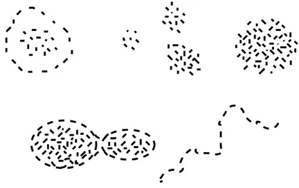
Clustering or unsupervised classification is a very difficult problem because data could form clusters with different shapes and sizes as shown in Figure 1.2. Cluster analysis is a very important and useful technique. The speed, reliability, and consistency of a clustering algorithm applied to a large amounts of data constitute strong reasons to use it in applications

(25)

1.4. Classification 7

such as data mining, information retrieval, image segmentation, signal compression and coding, and machine learning [12].

Figure 1.2: Different Shapes and Sizes of Clusters

There are hundreds of clustering algorithms and new clustering al-gorithms continue to appear. Most of these alal-gorithms are based on the following two popular clustering techniques: iterative square-error

partitional clustering and agglomerative hierarchical clustering [25]. Hi-erarchical techniques organize data in a nested sequence of groups which

can be displayed in the form of a tree. Square-error partitional algorithms try to find the partition which either minimizes the within–cluster scatter or maximizes the between–cluster scatter [27].

1.4 Classification

The task of classification is finding the best divider (separator) between two or more different classes, without or with minimum number of errors. In the simplest case there are only two different classes. Estimating a function f : Rd_{→ {0, 1}, is one possible formalization of this task, using}

(26)

input-output training data pairs which are assumed to be generated in-dependently and identically distributed (i.i.d.), according to an unknown probability distribution P (x, y), where

(x1, y1), . . . , (xn, yn) ∈ Rd× Y, Y = {0, 1}.

The objective is to define f which will correctly classify unseen examples (x, y). An example is assigned to the class 1 if f (x) ≥ 0 and to the class 0 otherwise. The test examples are assumed to be generated from the same probability distribution P (x, y) as the training data. A commonly used loss function measures the classification error is [8]

L(y, f (x)) =

½

0 if y = f (x)

1 if y 6= f (x) (1.8)

The best function f is the one that minimizing the expected error (risk)

R(f ) =

Z

L(y, f (x)) P (x, y) dx dy. (1.9) Learning then becomes the problem of finding the indicator function

f (x) (classifier) which minimizes the probability of misclassification,

equation (1.9), using only the training data. While the underlying prob-ability distribution P (x, y) is unknown, the risk cannot be minimized directly. So, users try to estimate a function that is close to the optimal one based on the available information.

The conditional densities for each class p(x|y = 0) and p(x|y = 1) are estimated via parametric density estimation and the ML inductive principle. These estimates will be denoted as p0(x, α∗) and p1(x, β∗),

re-spectively, to indicate that they are parametric functions with parameters chosen via ML. Prior probabilities are the probability of occurrence of each class, P (y = 0) and P (y = 1) are assumed to be known or estimated. Using Bayes theorem, it is possible to determine for a given observation x the probability that the observation belongs to each class, which is called posterior probabilities, that can be used to construct a discrimi-nant rule. This rule chooses the output class which has the maximum

(27)

1.4. Classification 9

posterior probability [14, 25]. Calculating the posterior probabilities for each class by using Bayes rule [8, 35]:

P (y = 0|x) = p0(x, α ∗_{)P (y = 0)} p(x) P (y = 1|x) = p1(x, β ∗_{)P (y = 1)} p(x) (1.10)

After calculating the posterior probabilities, x can be classified by using the following rule:

f (x) =    0 if p0(x, α∗)P (y = 0) > p1(x, β∗)P (y = 1) 1 otherwise (1.11) Equivalently, the rule can be written as

f (x) = I µ ln p1(x, β∗) − ln p0(x, α∗) + ln P (y = 1) P (y = 0) > 0 ¶ , (1.12)

where I( ) is the indicator function that takes the value 1 if its argu-ment is true and 0 otherwise. The class labels are denoted by {0 , 1}. Sometimes, for notational convenience, the class labels {–1 , +1} are used.

1.4.1 Multi–Class Classification

Multi–class classification is a central problem in machine learning. In this case a discrimination among several classes is required. The multi– class classification problem refers to assign each of the observations into one of k classes [11].

The most common approach to multi–class classification, the ”One versus All” (OvA) approach, makes direct use of ”standard” binary clas-sifiers to train the output labels. The OvA scheme assumes that for each class there exists a single (simple) separator between this class and all the other classes [1]. Another common approach, ”All versus All” (AvA), that assumes the existence of a separator between any two classes.

(28)

”One versus All” classifiers are usually implemented using a Winner-Take-All (WTA) strategy that associates a real–valued function with each class in order to determine class membership. Specifically, an example belongs to the class which assigns it the highest value (i.e., the ”winner”) among all classes. While it is known that WTA is an expressive classi-fier, it has limited expressivity when trained using the OvA assumption since OvA assumes that each class can be easily separated from the rest [18, 33]. An alternative interpretation of WTA is that each example pro-vides an order for the classes (sorted in descending order by the assigned values), where the ”winner” is the first class in this ordering. Therefore it’s natural to specify the ordering of the classes for an example directly, instead of implicitly through WTA.

1.5 Regression

Regression is the process of guessing or estimating a function from some example input–output pairs with little or no knowledge about the form of the function [11, 20, 25]. This means finding the best prediction of a random variable Y ∈ Rq _{(the output) by another random variable}

X ∈ Rd _{(the input). Assume q = 1, that will simplify the notation. In}

this framework, a predictor is a function f : Rd _{→ R.}

A common loss function for regression is the squared error (L2),

L(y, f (x)) = (y − f (x))2_. _(1.13)

Learning then becomes the problem of finding the function f (x)

(regres-sor) that minimizes the risk function R =

Z

(y − f (x))2_{p(x, y) dx dy,} _(1.14)

using only the training data. This risk functional measures the accuracy of the learning machine’s predictions of the system output [8, 11].

(29)

1.5. Regression 11

1.5.1 Linear Least Squares Regression

Linear least squares regression is so far the most widely used modeling method. The terms ”regression”, ”linear regression” or ”least squares” are synonymous of linear least square regression. For the input vector

x = (x1, x2, . . . , xp) we want to predict a real–valued output Y .

Linear least squares regression can be used to fit the data with any function of the form

f (x) = w0+ p X j=1 wjxj, (1.15) in which:

1. Each explanatory variable (input value xi) in the function is

mul-tiplied by an unknown parameter (wi).

2. There is at most one unknown parameter with no corresponding explanatory variable.

3. All the individual terms are summed to produce the final function value.

Since the unknown parameters (wi) are considered to be variables and

the explanatory variables (xi) are considered to be known coefficients

corresponding to those ”variables”, then the problem becomes a system (usually overdetermined) of linear equations that can be solved in the least squares sense for the values of the unknown parameters [12, 20]. Linear least squares regression also takes its name from the way the estimates of the unknown parameters are computed, The word ”linear” here describes the linearity of the model in terms of the wi not in terms

of the explanatory variables xi. The ”method of least squares” that is

used to obtain parameter estimates was independently developed in the late 1700’s and the early 1800’s by the mathematicians Karl Friedrich Gauss and Adrien Marie Legendre.

In the least squares method the unknown parameters are estimated by minimizing the sum of the squared deviations between the data and the model. If we have a set of training data (x1, y1) . . . (xn, yn) and we want

(30)

to estimate the parameters w. Each xi = (xi1, xi2, . . . , xip)T is a vector of

feature measurements for the ith case. Least squares estimation method picks the coefficients w = (w0, w1, . . . , wp)T that minimize the residual

sum of squares [25]. RSS(w) = n X i=1 (yi− f (xi))2 = n X i=1 (yi− w0− p X j=1 xijwj)2. (1.16)

For minimizing equation (1.16), we denote by X the n × (p + 1) matrix with each row an input vector (with a 1 in the first position), and similarly let y be the n–vector of outputs in the training set. Now we can rewrite the residual sum–of–squares as

RSS(w) = (y − Xw)T_{(y − Xw).} _(1.17)

This is a quadratic function in the p + 1 parameters. Differentiating with respect to w we obtain ∂RSS ∂w = −2X T_{(y − Xw)} ∂2_RSS ∂w∂wT = −2X T_X. (1.18)

Assuming that X is nonsingular and hence XT_{X is positive definite, we}

set the first derivative to zero

XT_{(y − Xw) = 0,} _(1.19)

to obtain the unique solution ˆ

w = (XT_X)−1_XT_y. _(1.20)

The fitted values at the training inputs are ˆ

y = X ˆw = XT_(XT_X)−1_XT_y, _(1.21)

where ˆyi = ˆf (xi). The matrix H = XT(XTX)−1X appearing in equation

(31)

1.6. Novelty Detection 13

1.5.2 Multiple Linear Regression

The linear model, equation (1.15), with p > 1 inputs is called the multiple

linear regression model. Multiple linear regression attempts to model

the relationship between two or more explanatory variables (X) and a response variable by fitting a linear equation to observed data [25]. Each value of the independent variable X is associated with a value of the dependent variable y. Instead of fitting a line to data, we are now fitting a plane (for 2 independent variables), a space (for 3 independent variables), etc.

1.6 Novelty Detection

An important ability of any signal classification scheme is detecting novel events. Several applications require the classifier to act as a detector rather than to be used as a classifier, that is, the requirement is to detect whether an input is part of the data that the classifier was trained on or it is in fact unknown. There are several important issues related to novelty detection; we can summarize them in terms of the following principles [34].

• Principle of robustness and trade–off: A novelty detection method

must be capable of robust performance on test data that maximizes the exclusion of novel samples while minimizing the exclusion of known samples. This trade-off should be predictable and under experimental control.

• Principle of uniform data scaling: In order to assist novelty

detec-tion, it should be possible that all test data and training data after normalization lie within the same range.

• Principle of parameter minimization: A novelty detection method

should aim to minimize the number of parameters that are in user set.

• Principle of generalization: The system should be able to generalize

(32)

• Principle of adaptability: A system that recognizes novel samples

during test should be able to use this information for retraining. • Principle of computational complexity: A number of novelty

detec-tion applicadetec-tions are online and therefore the computadetec-tional com-plexity of a novelty detection mechanism should be as low as pos-sible.

Statistical approaches are mostly based on modeling data on the basis of their statistical properties and using these information to estimate whether a test sample come from the same distribution or not. The simplest approach can be based on constructing a density function for data of a known class, and then assuming that data is computing the probability of a test sample belongs to that class. Another simple model is to find the distance of the sample from a class mean and threshold on the basis of how many standard deviations away the sample is. The distance measure itself can be Mahalanobis or some other probabilistic distance [12].

Two main approaches exist in the estimation of the probability den-sity function, parametric and non-parametric methods. The parametric

approach assumes that the data comes from a family of known

distribu-tions, such as the normal distribution and certain parameters are cal-culated to fit this distribution. In non-parametric methods the overall form of the density function is derived from the data as well as the pa-rameters of the model. As a result non-parametric methods give greater flexibility in general systems. Parametric methods for estimating the probability density function have sometimes limited use because they require extensive a priori knowledge of the problem. Non–parametric statistical approaches make no assumption on the form of data distribu-tion and therefore they are more flexible (though more computadistribu-tionally expensive) [20].

There are many applications where novelty detection is very impor-tant including signal processing, computer vision, pattern recognition, data mining, and robotics.

(33)

15

Chapter 2 Support Vector Machine and

Kernel Methods

In this chapter we introduce the Support Vector Machine (SVM) classifi-cation technique, and show how it leads to the formulation of a Quadratic Programming (QP) problem in a number of variables that is equal to the number of data points. We will start by reviewing the classical

Empiri-cal Risk Minimization (ERM) approach, and by showing how it naturally

leads, through the theory of VC bounds, to the idea of Structural Risk

Minimization (SRM), which is a better induction principle, and how SRM

is implemented by SVM. Also we discuss the principles of kernel trans-formations, which provide the main building blocks of Support Vector Machine.

2.1 Support Vector Machines

Support vector machines (SVM) are a set of related supervised learning methods used for classification and regression. They belong to a family of generalized linear classifiers. This family of classifiers has both abilities: to minimize the empirical classification error and to maximize the geometric margin. Hence it is also known as maximum margin classifier

approach [1].

An important feature of the SVM approach is that the related

(34)

timization problems are convex because of Mercer’s conditions on the kernels [12]. Consequently, they haven’t local minima. The reduced number of non–zero parameters gives the ability to distinguish between these system and other pattern recognition algorithms, such as neural networks [11].

2.1.1 VC–Dimension

The Vapnik–Chernovenkis (VC) dimension is a scalar value that measures the capacity of a hypothesis space. Capacity is a measure of complexity and the expressive power, richness or flexibility of a set of functions.

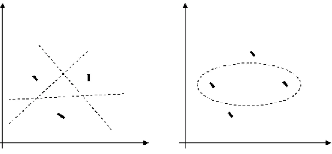
Figure 2.1: VC–Dimension Illustration

To give a simple VC–dimension example as shown in Figure 2.1, there are 23 _{= 8 ways of assigning 3 points to two classes. For the displayed}

points in R2_{, all 8 possibilities can be realized using one separating}

hy-perplane, in other words, the function class can shatter 3 points, where

shattering is ”if n samples can be separated by a set of indicator

(35)

2.1. Support Vector Machines 17

by the set of functions”. This would not work if we were given 4 points, no matter how we placed them. Therefore, the VC–dimension of the class of separating hyperplanes in R2 _{is 3. In general, the set of linear}

indicator functions in n dimensional space has a VC–dimension equal to

n + 1 [18, 25, 35].

2.1.2 Empirical Risk Minimization

The task of learning from examples can be formulated in the following way:

Given a set of decision functions

{fλ(x) : λ ∈ Λ}, fλ : Rd → {−1, +1}

where Λ is a set of abstract parameters, and a set of examples (x1, y1), . . . , (xl, yl), xi ∈ Rd, yi ∈ {−1, +1}

drawn from an unknown distribution P (x, y), we want to find a function

fλ∗ which provides the smallest possible value for the expected risk:

R(λ) =

Z

|fλ(x) − y| P (x, y) dx dy (2.1)

the function fλ are usually called hypothesis, and the set {fλ(x) : λ ∈ Λ}

is called hypothesis space and denoted by H. Therefore the measure of how ”good” the hypothesis in predicting the correct label y for a point x is called or known as the expected risk.

It is not possible in general to compute and then to minimize the expected risk R(λ), because the probability distribution P (x, y) is un-known. However, since P (x, y) is sampled, it’s possible to compute the stochastic approximation of R(λ), and this is called empirical risk:

Remp(λ) = 1 n n X i=1 |fλ(xi) − yi| (2.2)

The empirical risk minimization principle is ”if Remp converges to R,

the minimum of Remp may converge to the minimum of R”. If

(36)

Empirical Risk Minimization principle does not allow us to make any in-ference based on the data set, and it is therefore said to be not consistent [11].

A typical uniform Vapnik and Chervonenkis bound, which holds with probability 1 − η has the following form:

R(λ) ≤ Remp(λ) + s h(ln2n h + 1) − ln η 4 n ∀λ ∈ Λ (2.3)

where h is the VC–dimension of fλ. From this bound it is clear that, in

order to achieve small expected risk, that is good generalization perfor-mances, both the empirical risk and the ratio between the VC–dimension and the number of data points has to be small. Since the empirical risk is usually a decreasing function of h, it turns out that, for a given num-ber of data points, there is an optimal value of the VC–dimension. The bound of Vapnik and Chervonenkis (equation 2.3) suggests that the Em-pirical Risk Minimization principle can be replaced by a better induction principle.

2.1.3 Structural Risk Minimization

The technique of Structural Risk Minimization (SRM) has been devel-oped by Vapnik to overcome the problem of choosing an appropriate VC–dimension. It is clear from equation (2.3) that a small value of the empirical risk does not necessarily gives a small value of the expected risk [49]. The principle of Structural Risk Minimization is based on the observation that, in order to make the expected risk small, both sides in equation (2.3) should be small, therefore; both the VC–dimension and the empirical risk should be minimized at the same time [2, 25, 46].

In order to implement the SRM principle we need a nested structure of hypothesis spaces as shown in Figure 2.2

H1 ⊂ H2 ⊂ . . . ⊂ Hn⊂ . . .

with the property that h(l) ≤ h(l + 1) where h(l) is the VC–dimension of the set Hl [5].

(37)

H

1

H

2

H

n

Figure 2.2: Structure of a nested Hypothesis spaces

The SRM principle is clearly well founded mathematically, but it can be difficult to implement for the following two reasons [8]:

1. It is often difficult to find the VC–dimension for a hypothesis space

Hl, since not for all models and machines it is known how to

cal-culate this.

2. Even if it is possible to compute hl (or a bound on it) of Hlit is not

trivial to solve the optimization problem that is given by equation (2.3).

In most cases SRM has to be done by simply training a series of ma-chines, one for each subset, and then choosing Hl that gives the lowest

risk bound. Therefore the implementation of this principle is not easy, because it is important to control the VC–dimension of a learning tech-nique during the training phase. The SVM algorithm achieves this goal, minimizing a bound on the VC–dimension and the number of training errors at the same time [2].

(38)

2.1.4 The Optimal Separating Hyperplane

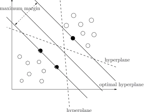
A separating hyperplane is a linear function that has the ability of sep-arating the training data without error as shown in Figure 2.3. Suppose that the training data consists of n samples (x1, y1), . . . , (xn, yn), x ∈

Rd_{, y ∈ {+1, −1} that can be separated by a hyperplane decision}

func-tion

D(x) = hw . xi + b, (2.4) with appropriate coefficients w and b [8, 11, 25, 50]. Notice that the problem is ill-posed because the solution may be not unique and then some constraint has to be imposed to the solution to make the problem

well-posed [13].

hyperplane

hyperplane maximum margin

optimal hyperplane

Figure 2.3: Separating hyperplanes in a two–dimensional space. An op-timal hyperplane with a maximum margin. The dashed lines are not optimal hyperplanes

(39)

A separating hyperplane satisfies the constraints that define the sep-aration of the data samples:

hw . xii + b ≥ +1 if yi = +1

hw . xii + b ≤ −1 if yi = −1, i = 1, 2, . . . , n.

(2.5) Or in more compact form (notation)

yi[hw . xii + b] ≥ 1, i = 1, 2, . . . , n. (2.6)

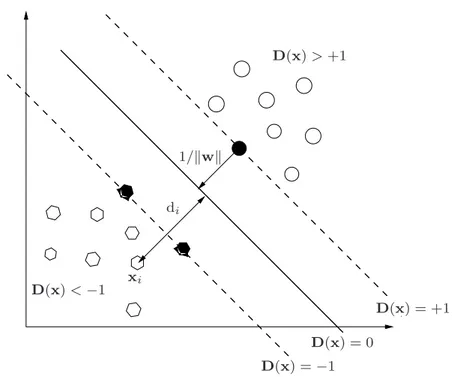
For a given separable training data set, all possible separating hy-perplanes can be represented in the form (2.6). The formulation of the separating hyperplanes allows us to solve the classification problem di-rectly. It does not require estimation of density as an intermediate step [1]. When D(x) is equal to 0, this hyperplane is called separating

hyper-plane as shown in Figure 2.4.

Let di be the signed distance of the point xi from the separating

hyperplane

di =

hw . xii + b

kwk (2.7)

where the symbol kwk denotes the norm of w. From this equation follows that

dikwk = hw . xii + b

and using the constraints (2.6), we have

yidikwk ≥ 1.

So for all xi the following inequality holds:

1

kwk ≤ yidi. (2.8)

Notice that yidiis always positive quantity. Moreover, 1/kwk is the lower

bound on the distance between the points xi and the separating

hyper-plane (w, b). The purpose of the ”1” in the righthand side of inequality (2.6) for establishing a one–to–one correspondence between separating

(40)

D(x) = +1 xi D(x) > +1 D(x) = 0 D(x) = −1 D(x) < −1 di 1/kwk

Figure 2.4: Optimal separating hyperplane in a two–dimensional space and the distance between it and any sample

hyperplanes and their parametric representation. This is done through the notion of canonical representation of a separating hyperplane [44].

The optimal hyperplane is given by maximizing the margin, γ, subject to the constraints (2.6). The margin is given by [11, 51],

γ(w, b) = min i:yi=−1 di+ min i:yi=+1 di = min i:yi=−1 hw . xii + b kwk + mini:yi=+1 hw . xii + b kwk = 1 kwk µ min i:yi=−1 (hw . xii + b) + min i:yi=+1 (hw . xii + b) ¶ = 2 kwk. (2.9)

(41)

2.2. Support Vector Classification 23

Thus the optimal hyperplane is the one that minimizes Φ(w) = 1

2kwk

2_. _(2.10)

Because Φ(w) is independent of b, changing b moves it in the normal direction to itself, and hence the margin remains unchanged but the hyperplane is no longer optimal in that it will be nearer to one class than the other.

Now we discuss why minimizing (2.10) is equivalent to implementing the SRM principle. Suppose that the following bound holds,

kwk ≤ A, (2.11)

then from (2.8)

d ≥ 1

A, (2.12)

this is equivalent to placing spheres of radius 1

A around each data points

and consider only the hyperplanes that do not intersect any of the spheres, and intuitively it can be seen in Figure 2.5 how this reduces the possible hyperplanes, and hence the capacity [37].

The VC–dimension, h, of the set of canonical hyperplanes in d– dimensional space is bounded by,

h ≤ min{dR2A2e, d} + 1, (2.13) where R is the radius of the hypersphere enclosing all the data points. Hence minimizing (2.10) is equivalent to minimizing an upper bound on the VC–dimension [8, 44, 50].

2.2 Support Vector Classification

In this section we describe the mathematical derivation of the Support

Vector Machine (SVM) developed by Vapnik. The Support Vector

Ma-chine (SVM) implements the idea of mapping the input vectors x into the high–dimensional feature space F through some nonlinear mapping,

(42)

1/A

Figure 2.5: Constraining the Canonical Hyperplanes

chosen a priori. In this space, an optimal separating hyperplane is con-structed [50].

The technique is introduced by steps: at first consider the simplest case, i.e. a linear classifier and a linearly separable problem; then a linear classifier and a nonseparable problem, and the last one which is the most interesting and useful, nonlinear classifier and nonseparable problem.

2.2.1 Linear Classifier and Linearly Separable

Problem

In this section we consider the case where the data set is linearly

sep-arable, and we want to find the ”best” hyperplane that separates the

data. In other words finding the pair (w, b) satisfying the constraints in equation (2.6). The hypothesis space in this case is the set of functions

(43)

given by

fw,b = sgn(hw . xi + b). (2.14)

Because the set of examples are linearly separable, the goal of the SVM is to find, among the Canonical Hyperplanes that correctly classify the data, the one at minimum norm. Minimizing kwk2 _{(in this case of linear}

separability) is equivalent to finding the separating hyperplane that max-imizes the distance between the two convex hulls (of the two classes of training data), measured along the line perpendicular to the hyperplane, as shown in Figure 2.6. yi= −1 yi= +1 {x:(w.x)+b=+1} {x:(w.x)+b=0} {x:(w.x)+b=-1}

Figure 2.6: The optimal hyperplane is orthogonal to the shortest line connecting the convex hulls of the two classes (dotted)

(44)

The solution to the optimization problem of equation (2.10) under the constraints of equation (2.6) consists of (d + 1) parameters. For data of moderate dimension d, this problem can be solved using Quadratic Programming (QP) [1].

For very high–dimensional spaces it is not practical to solve the prob-lem in the present form

min w,b Φ(w) = 1 2kwk 2 subject to yi[hw . xii + b] ≥ 1, i = 1, 2, . . . , n. (2.15)

However, this problem can be translated into a dual form that can be better tackled. In case of convexity (as in our problem) solving the dual problem is equivalent to solving the original. For the optimal hyperplane problem it turns out that the size of dual optimization problem scales with the number of samples n and not the dimensionality d. The solution to this problem is given by the saddle point of the Lagrange function (Lagrangian), L(w, b, α) = 1 2kwk 2₋ n X i=1 αi{ yi[hw . xii + b] − 1 }, (2.16)

where αi are the Lagrange multipliers. The function should be minimized

with respect to w, b and maximized with respect to αi ≥ 0. Classical

Lagrangian duality enables the primal problem, equation (2.16), to be transformed to its dual problem, which is easier to solve. The dual prob-lem is given by,

max α W(α) = maxα µ min w,b L(w, b, α) ¶ . (2.17)

The Karush–Kuhn–Tucker (KKT) conditions play a central role in both the theory and practice of constrained optimization. For the primal

(45)

problem above, the KKT conditions may be stated [11, 15, 49, 50]:

∂L ∂b = 0 ⇒ n X i=1 αiyi = 0 ∂L ∂w = 0 ⇒ w = n X i=1 αiyixi, (2.18)

which are satisfied at the minimum of Lagrangian L. The KKT condi-tions are satisfied at the solution of any constrained optimization problem (convex or not), with any kind of constraints, provided that the intersec-tion of the set of feasible direcintersec-tions with the set of descent direcintersec-tions co-incides with the intersection of the set of feasible directions for linearized constraints with the set of descent directions. Furthermore, the problem for SVM is convex (a convex objective function, with constraints which give a convex feasible region), the KKT conditions are necessary and

suf-ficient for w, b, and α to be a solution. Thus solving the SVM problem is

equivalent to finding a solution to the KKT conditions [1, 5, 25]. Hence from (2.16), (2.17) and (2.18), the dual problem is

max α W(α) = maxα Ã _n X i=1 αi− 1 2 n X i=1 n X j=1 αiαjyiyjhxi . xji ! , (2.19)

and hence the solution to the problem is given by,

α∗ _{= arg min} α 1 2 n X i=1 n X j=1 αiαjyiyjhxi . xji − n X i=1 αi, (2.20)

subject to the constraints

n X i=1 yiαi = 0, αi ≥ 0, i = 1, 2, . . . , n. (2.21)

(46)

multipliers, and the optimal separating hyperplane is given by, w∗ ₌ n X i=1 αiyixi (2.22) b∗ _{= −}1 2hw ∗ _{. (x} r+ xs)i, (2.23)

where xr and xs are any support vector (points have α > 0) from each

class satisfying,

αr, αs > 0, yr = −1, ys = +1. (2.24)

By linearity of the dot product and (2.21), the decision function (hard classifier), as shown in (2.14) can then be written as:

f (x) = sgn Ã _n X i=1 yiα∗ihx . xii + b∗ ! . (2.25)

2.2.2 The Soft Margin Hyperplane: Linearly

Non-separable Problem (C–SVM)

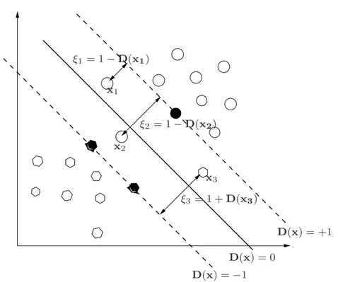
So far the discussion has been restricted to the case of linearly separable training data. But for the data that can not be separated without error, it would be better to separate the data with a minimal number of errors. This means finding an optimal hyperplane (i.e., with maximal margin) for the training data points that are accurately separated, while it is not possible to satisfy all the constraints in problem (equation 2.15). This corresponds to some data points that fall within the margin or on the wrong side of the decision boundary [8]. Note that the definition of nonseparable differs from misclassification, which occurs when a data point only falls on the wrong side of the decision boundary as shown in Figure 2.7.

Non negative slack variables ξi, i = 1, . . . , n, can be introduced to

quantify the nonseparable data in the defining condition of the hyper-plane [25]. The optimization problem is now posed so as to minimize the classification error as well as minimizing the bound on the VC–dimension

(47)

2.2. Support Vector Classification 29 D(x) = +1 D(x) = 0 D(x) = −1 x3 ξ2= 1 − D(x2) x1 ξ1= 1 − D(x1) x2 ξ3= 1 + D(x3)

Figure 2.7: Nonseparable case, slack variables are defined that correspond to the deviation from the margin borders.

of the classifier. The constraints of equation (2.6) are modified for the nonseparable case as follows,

yi[hw . xii + b] ≥ 1 − ξi, i = 1, 2, . . . , n. (2.26)

For training sample xi, the slack variable ξi is the deviation from

the margin border corresponding to the class of yi (i.e., the margin

bor-der defined by D(x_i) = yi); as shown in Figure 2.7. According to the

definition, slack variables greater than zero correspond to nonseparable points, while slack variables greater than one correspond to misclassified samples [41]. Minimizing the number of nonseparated points is a difficult combinatorial optimization problem. Hence we resort to the

(48)

minimiza-tion of Q(ξ) = n X i=1 ξi, (2.27)

The function (2.27) only approximates the number of nonseparable sam-ples. The hyperplane that minimizes (2.27) subject to the constraint (2.26) and using the structure

Sk = {hw . xi + b : kwk2 ≤ ck}, (2.28)

is called the soft margin hyperplane. The optimization problem that finds the soft margin hyperplane is convex, this means that each (local) minimum is also a global minimum [36].

The generalized optimal separating hyperplane for the case of linearly nonseparable classes can be seen as the solution of the following problem:

min w,b,ξ Φ(w, ξ) = 1 2kwk 2_{+ C} n X i=1 ξi subject to yi[hw . xii + b] ≥ 1 − ξi, i = 1, 2, . . . , n ξi ≥ 0, i = 1, 2, . . . , n (2.29)

where C is a positive constant number which can be regarded as a

reg-ularization parameter, which determines the trade off between accuracy

on the training set (i.e. smallP_iξi) and margin width (i.e. small kwk2).

Increasing C means giving more importance to the errors on the train-ing set when the optimal hyperplane is determined. The solution to the optimization problem (2.26) is given by the saddle point (the point that minimizes the functional with respect to w and b and maximizes it with respect to α) of the Lagrangian

L(w, b, α, ξ, β) = 1 2kwk 2_{+ C} n X i=1 ξi− n X i=1 αi{ yi[hw . xii + b] −1 + ξi} − n X i=1 βiξi, (2.30)

(49)

where α and β are the Lagrange multipliers. The Lagrangian has to be minimized with respect to w, b, and ξi, and maximized with respect to

αi ≥ 0 and βi ≥ 0.

Classical Lagrangian duality enables the primal problem (equation 2.30) to be transformed into its dual form. The dual problem is given by [1, 11, 25, 50], max α W(α, β) = maxα, β µ min w,b,ξL(w, b, α, ξ, β) ¶ , (2.31)

the minimum with respect to w, b and ξ of the Lagrangian, L, is given by, ∂L ∂b = 0 ⇒ n X i=1 αiyi = 0 ∂L ∂w = 0 ⇒ w = n X i=1 αiyixi ∂L ∂ξ = 0 ⇒ αi+ βi = C. (2.32)

Hence from equations (2.30), (2.31) and (2.32), the dual problem is, max α W(α) = maxα Ã n X i=1 αi− 1 2 n X i=1 n X j=1 αiαjyiyjhxi . xji ! , (2.33)

and hence the solution to the problem is given by,

α∗ _{= arg min} α 1 2 n X i=1 n X j=1 αiαjyiyjhxi . xji − n X i=1 αi, (2.34)

subject to the constraints

0 ≤ αi ≤ C, i = 1, 2, . . . , n n X i=1 yiαi = 0. (2.35)

(50)

This optimization problem differs from the optimization problem for the separable case only with the inclusion of a bound C in the constraint (2.35). This parameter introduces additional capacity control within the classifier. C can be directly related to a regularization parameter, but ultimately C must be chosen to reflect the knowledge of the noise on the data [21].

Similarly to the separable case, the points xi for which αi > 0 are

termed support vectors. The main difference is that we must distin-guish between the support vectors for which αi < C and those for which

αi = C. In the first case, when ξi = 0 the support vectors lie at a distance

1/kwk from the Optimal Separating Hyperplane (OSH). These support vectors are termed margin vectors as we know before. The support vec-tors for which αi = C, instead, are misclassified points (if ξi > 1), points

correctly classified but closer than 1/kwk from the OSH (if 0 < ξi ≤ 1),

or, in some degenerate cases, even points lying on the margin (if ξi = 0)

[8, 44].

An example of generalized OSH with the relative margin vectors and errors is shown in Figure 2.7. All the points that are not support vectors are correctly classified and lie outside the margin strip.

2.3 Kernel Functions and Nonlinear SVM

Kernel representations offer an alternative solution by projecting the data into a high dimensional feature space to increase the computational power of the linear learning machines. The use of linear machines in the dual representation makes it possible to perform this step explicitly. The advantage of using the machines in the dual representation derives from the fact that in this representation the number of tunable parameters does not depend on the number of attributes being used. By replacing the inner product with an appropriately chosen ’kernel’ function, one can implicitly perform a nonlinear mapping to a high dimensional feature space without increasing the number of tunable parameters, provided the kernel computes the inner product of the feature vectors corresponding to the two inputs [11].

(51)

2.3. Kernel Functions and Nonlinear SVM 33

2.3.1 Kernel Feature Space

The quantities introduced to describe the data are usually called

at-tributes. The task of choosing the most suitable representation is known

as feature selection. The space X is referred to as the input space, while

F = {φ(x) : x ∈ X} is called the feature space [12]. Feature mapping

from a two dimensional input space to a two dimensional feature space, is shown in Figure 2.8, where the data cannot be separated by a linear function in the input space, but can be in the feature space [35].

feature space input space

φ

Figure 2.8: A feature map can simplify the classification task.

There are different approaches for feature selection, one of them tries to identify the smallest set of features that still has the important infor-mation contained in the original attributes. This is known as

dimension-ality reduction,

x = (x1, . . . , xn) 7→ φ(x) = (φ1(x), . . . , φd(x)), d < n,

and can be very beneficial as both computational and generalization per-formance can degrade as the number of features grows, a phenomenon sometimes referred to as the curse of dimensionality. Dimensionality re-duction can sometimes be performed by simply removing features corre-sponding to directions in which the data have low variance, though there

(52)

is no guarantee that these features are not important for performing the target classification [11].

Feature selection should be viewed as a part of the learning process itself, and should be automated as much as possible. Therefore for learn-ing nonlinear relations with a linear machine, it’s very important to select a set of nonlinear features and rewrite the data in the new representa-tion. This is equivalent to apply a fixed nonlinear mapping of the data to a feature space, in which the linear machine can be used. Hence, the decision function (2.14) becomes

f (x) =

m

X

i=1

wiφi(x) + b,

where φ : X → F is a nonlinear map from the input space to some feature space, and the number of terms in the summation (m) depends on the dimensionality of the feature space. This mean building non–linear machines consist of two steps:

• STEP 1: Transforming the data into a feature space F by using a fixed nonlinear mapping.

• STEP 2: Using a linear machine to classify the data in the feature space.

The important property of linear learning machines is that they can be expressed in a dual form. Therefore the hypothesis can be expressed as a linear combination of the training points, so that the decision rule can be evaluated using just inner products between the test point and the training points:

f (x) =

n

X

i=1

αiyihφ(xi) . φ(x)i + b. (2.36)

If there is a way to compute the inner product αiyihφ(xi) . φ(x)i in

feature space directly as a function of the original input points, it becomes possible to combine the two steps needed to build a nonlinear learning machine, and this direct computation method is called kernel function

(53)

[12]. Through this kernel technique, the value of the kernel function can be computed over a sample set instead of the dot product in a high– dimensional feature space [47]. The kernel function will take the symbol K, such that K(x, z) = hφ(x).φ(z)i, and hence, equation (2.36) can be rewritten in this form

f (x) =

n

X

i=1

αiyiK(xi, x) + b. (2.37)

The expansion of the inner product (2.36) in the dual representation allows the construction of decision functions that are nonlinear in the input space. It also makes computationally possible the creation of very high–dimensional feature space, since no direct manipulation is required. Common classes of basis functions used for learning machines cor-respond to different choices of kernel functions for computing the inner product. Below are several common classes of multivariate approximat-ing functions and their inner product Kernels:

Polynomials of degree q have inner product kernel

K(x, z) = (hx . zi + 1)q_, _(2.38)

which is a popular mapping method for nonlinear modeling Gaussian Radial Basis Functions of the form,

K(x, z) = exp(−kx − zk2

2σ2 ), (2.39)

where σ defines the width.

Exponential Radial Basis Function of the form K(x, z) = exp(−kx − zk

2σ2 ), (2.40)

produces a piecewise linear solution which can be attractive when dis-continuities are acceptable.

(54)

Multi–Layer Perceptron (Sigmoid) has a kernel representation

K(x, z) = tanh (vhx . zi + a), (2.41)

for parameter values scale, v, and offset, a, selected so that the kernel satisfies Mercer’s conditions. Here the Support Vectors (SV) correspond to the first layer and the Lagrange multipliers to the weights.

2.3.2 Non Linear Classifier and Non Separable

Problem (C–SVM)

In the case where a linear boundary is unsuitable, the SVM can map the input vector, x, into a high dimensional feature space, z. By choosing a nonlinear mapping a priori, the SVM constructs an optimal separat-ing hyperplane in this higher dimensional space, Figure 2.9 shows the mapping process.

Output Space

Feature Space Input Space

Figure 2.9: Mapping the input space into a high dimensional feature space.

There are some restrictions on the nonlinear mapping that can be employed, but it turns out, surprisingly, that most commonly employed

(55)

functions are acceptable. Among acceptable mappings are polynomials, radial basis functions and certain sigmoid functions as explained in the last section. The optimization problem of equation (2.20) becomes,

α∗ = arg min α 1 2 n X i=1 n X j=1 αiαjyiyjK(xi, xj) − n X i=1 αi, (2.42)

where K(xi, xj) is the kernel function performing the nonlinear mapping

into feature space , and the constraints are unchanged,

n X i=1 yiαi = 0. 0 ≤ αi ≤ C, i = 1, 2, . . . , n. (2.43)

Solving equation (2.42) with constraints equation (2.43) determines the Lagrange multipliers, and a hard classifier implementing the optimal sep-arating hyperplane in the feature space is given by,

f (x) = sgn Ã X i∈SVs yiαiK(xi, x) + b ! , (2.44) where (w∗. x) = n X i=1 yiαiK(xi, x).

In addition, to compute the threshold b, we consider that for the support vectors {xi, i ∈ SV }, where SV is the set of index of support vectors, the

corresponding {ξi, i ∈ SV } are all zeros due to the Kuhn–Tucker dual

condition in a dual optimization problem. As a result, we have X

i∈SV

yiαiK(xi, xj) + b = yj, j ∈ SV. _(2.45)

In order to have robust performance and reduce the effect of computa-tional errors and noises, we can sum (2.45) over all support vectors and

(56)

solve for the threshold b = 1 NSV [X j∈SV yj− X i,j∈SV yiαiK(xi, xj)], (2.46)

where NSV is the number of support vectors. All the results on the

linear case can also be directly applied to nonlinear cases through using an appropriate kernel K in place of the Euclidean dot product in feature space. By use of this technique, we can easily compute the dot product in the feature space from the input space [47].

2.4 Support Vector Regression

The SVM approach can be fruitfully applied to regression problems. In this case we suppose that a training set of couples (yi, xi), i = 1, 2, . . . , n, xi ∈

Rd_{, y}

i ∈ R is given, corresponding to an unknown function f : Rd → R.

i.e. yi = f (xi).

Then the SVM approach consists basically in solving min kwk2+ C n X i=1 (ξ_i2+ ˆξ2_i) subject to (hw.xii + b) − yi ≤ ε + ξi, i = 1, 2, . . . , n, yi− (hw.xii + b) ≤ ε + ˆξi, i = 1, 2, . . . , n, ξi, ˆξi ≥ 0, i = 1, 2, . . . , n (2.47)

where we have introduced two slack variables, one for exceeding the target value by more than ε, and the other for being more than ε below the target.

Figure 2.10 shows an example of a one dimensional linear regression function with an ε–insensitive band. The variables ξ measure the cost of the errors on the training points, which have the value equal to zero for all the points inside the band. Figure 2.11 shows a similar situation for a non–linear regression function [11].

(57)

2.4. Support Vector Regression 39

Figure 2.10: The insensitive band for a one dimensional linear regression problem

Figure 2.11: The insensitive band for a one dimensional non–linear re-gression problem

Classification models and algorithms in application of multi-sensor systems to detection and identification of gases