Universit`a Politecnica delle Marche
Scuola di Dottorato di Ricerca in Scienze dell’Ingegneria Curriculum in Ingegneria Informatica, Gestionale e dell’Automazione
Processing and visualization of
multi-source data in
next-generation geospatial
applications
Ph.D. Dissertation of:
Mirco Sturari
Advisor:Prof. Primo Zingaretti
Curriculum Supervisor: Prof. Francesco Piazza
Universit`a Politecnica delle Marche
Scuola di Dottorato di Ricerca in Scienze dell’Ingegneria Facolt`a di Ingegneria
alla mia famiglia:
Selene, Marco Augusto, Sebastiano e Costantino
Ringraziamenti
Questo lavoro di tesi `e il frutto di un’esperienza di 3 anni, all’interno del gruppo di ricerca VRAI, in cui mi sono sentito da subito apprezzato e valoriz-zato.
La mia famiglia, dai miei genitori ai miei figli, ma in particolare mia moglie Selene, mi ha sempre appoggiato nelle scelte, anche se mi hanno portato a dedicare sempre pi`u tempo alla ricerca. Un grazie per avermi permesso di portare a termine questa esperienza come volevo io, nel migliore dei modi, compensando le mie frequenti mancanze nella vita familiare.
Un grazie al mio dirigente in Regione Marche, Arch. Bucci, che mi ha consen-tito di intraprendere questo progetto di crescita rispettando le mie aspirazioni, e al mio collega e amico Massimiliano, l’unica persona valida e professionale in grado di reggere da solo il sistema informativo territoriale.
Un grazie al Prof. Zingaretti e al Prof. Frontoni che mi hanno offerto la possibilit`a di intraprendere il percorso del dottorato di ricerca. Primo, nel suo modo diretto e netto, ha sempre cercato di portare il rigore metodologico nella mia ricerca scientifica. Emanuele, nel suo modo a volte sin troppo visionario, ha sempre cercato di stimolare ed evidenziare l’innovativit`a in quello facevo.
Un grazie a tutti i colleghi con cui ho avuto il piacere di lavorare. Adriano, un esempio di dedizione alla ricerca, all’insegnamento e al lavoro, diventato un amico con cui ho realizzato alcuni dei progetti pi`u interessanti e impeg-nativi della mia carriera. Marina, un’altra collega che `e diventata un’amica, in grado di svegliarsi con il sorriso, contagiarti con la sua solarit`a ed essere allo stesso tempo un’ottima e instancabile ricercatrice. Roberto, che ormai considero come un fratello, con cui ho formato un’accoppiata che ha prodotto ottimi risultati scientifici sia dal punto di vista tecnico che innovativo: The Power of ... Dinamico Duo!
Ancona, October 2017
Sommario
Le applicazioni geospaziali di nuova generazione come dati non usano sem-plicemente punti, linee e poligoni, ma oggetti complessi o evoluzioni di fenomeni che hanno bisogno di tecniche avanzate di analisi e visualizzazione per essere compresi. Le caratteristiche di queste applicazioni sono l’uso di dati multi-sorgente con diverse dimensioni spaziali, temporali e spettrali, la visualizzazione dinamica e interattiva con qualsiasi dispositivo e quasi ovunque, anche sul campo.
L’analisi dei fenomeni complessi ha utilizzato fonti dati eterogenee per forma-to/tipologia e per risoluzione spaziale/temporale/spettrale, che rendono prob-lematica l’operazione di fusione per l’estrazione di informazioni significative e immediatamente comprensibili. L’acquisizione dei dati multi-sorgente pu`o avvenire tramite diversi sensori, dispositivi IoT, dispositivi mobili, social me-dia, informazioni geografiche volontarie e dati geospaziali di fonti pubbliche.
Dato che le applicazioni geospaziali di nuova generazione presentano nuove caratteristiche, per visualizzare i dati grezzi, i dati integrati, i dati derivati e le informazioni `e stata analizzata l’usabilit`a di tecnologie innovative che ne consentano la visualizzazione con qualsiasi dispositivo: dashboard interattive, le viste e le mappe con dimensioni spaziali e temporali, le applicazioni di Aug-mented e Virtual Reality.
Per l’estrazione delle informazioni in modo semi-automatico abbiamo impie-gato varie tecniche all’interno di un processo sinergico: segmentazione e identifi-cazione, classifiidentifi-cazione, rilevamento dei cambiamenti, tracciamento e clustering dei percorsi, simulazione e predizione. All’interno di un workflow di elabo-razione, sono stati analizzati vari scenari e implementate soluzioni innovative caratterizzate dalla fusione di dati multi-sorgente, da dinamicit`a e interattiv`a. A seconda dell’ambito applicativo le problematiche sono differenziate e per ciascuno di questi sono state implementate le soluzioni pi`u coerenti con suddette caratteristiche.
In ciascuno scenario presentato sono state trovate soluzioni innovative che hanno dato buoni risultati, alcune delle quali in nuovi ambiti applicativi: (i) l’integrazione di dati di elevazione e immagini multispettrali ad alta risoluzione per la mappatura Uso del Suolo / Copertura del Suolo, (ii) mappatura con il contributo volontario per la protezione civile e la gestione delle emergenze (iii) la fusione di sensori per la localizzazione e il tracciamento in ambiente
retail, (iv) l’integrazione dei dati in tempo reale per la simulazione del traffico nei sistemi di mobilit`a, (v) la combinazione di informazioni visive e di nuvole di punti per la rilevazione dei cambiamenti nell’applicazione della sicurezza ferroviaria. Attraverso questi esempi, i suggerimenti potranno essere applicati per realizzare applicazioni geospaziali anche in ambiti diversi.
Nel futuro sar`a possibile aumentare l’integrazione per realizzare piattaforme data-driven come base per sistemi intelligenti: un’interfaccia semplice per l’utente che metta a disposizione funzionalit`a avanzate di analisi costruite su algoritmi affidabili ed efficienti.
Abstract
Next-generation geospatial applications as data do not simply use dots, lines, and polygons, but complex objects or evolution of phenomena that need ad-vanced analysis and visualization techniques to be understood. The features of these applications are the use of multi-source data with different spatial, temporal and spectral dimensions, dynamic and interactive visualization with any device and almost anywhere, even in the field.
Complex phenomena analysis has used heterogeneous data sources for for-mat/typology and spatial/temporal/spectral resolution, which challenging com-bining operation to extract meaningful and immediately comprehensible infor-mation.
Multi-source data acquisition can take place through various sensors, IoT devices, mobile devices, social media, voluntary geographic information and geospatial data from public sources. Since next-generation geospatial applica-tions have new features to view raw data, integrated data, derived data, and information, wh have analysed the usability of innovative technologies to en-able visualization with any device: interactive dashboards, views and maps with spatial and temporal dimensions, Augmented and Virtual Reality appli-cations.
For semi-automatic data extraction we have used various techniques in a synergistic process: segmentation and identification, classification, change de-tection, tracking and path clustering, simulation and prediction. Within a processing workflow, various scenarios were analysed and implemented innova-tive solutions characterized by the fusion of multi-source data, dynamism and interactivity.
Depending on the application field, the problems are differentiated and for each of these the most coherent solutions have been implemented with the aforementioned characteristics. Innovative solutions that have yielded good results have been found in each scenario presented, some of which are in new applications: (i) integration of elevation data and multispectral high-resolution images for Land Use/Land Cover mapping, (ii) crowd-mapping for civil pro-tection and emergency management, (iii) sensor fusion for indoor localization and tracking, (iv) integration real-time data for traffic simulation in mobility systems, (v) mixing visual and point cloud informations for change detection on railways safety and security application.
Through these examples, given suggestions can be applied to create geospa-tial applications even in different areas. In the future, integration can be en-hanced to build data-driven platforms as the basis for intelligent systems: a user-friendly interface that provides advanced analysis capabilities built on re-liable and efficient algorithms.
Contents
1 Context 1
1.1 Geospatial applications . . . 1
1.2 Structure of the thesis . . . 4
2 State of art 5 2.1 Geospatial data sources . . . 5
2.2 Integration of multi-source data . . . 8
2.3 Visualization . . . 9
3 Materials and methods 13 3.1 Workflow . . . 13
3.2 Processing . . . 16
3.2.1 Segmentation and Identification . . . 16
3.2.2 Classification . . . 18
3.2.3 Change Detection . . . 22
3.2.4 Tracking and Path Clustering . . . 25
3.2.5 Simulation and Prediction . . . 28
3.3 Visualization . . . 31
3.3.1 Web/Map dashboard . . . 31
3.3.2 3D Point Cloud . . . 33
3.3.3 360◦Image and Video . . . . 33
3.3.4 Augmented Reality . . . 35
4 Results and discussion 39 4.1 Integrating elevation data and multispectral high-resolution im-ages for Land Use/Land Cover mapping . . . 39
4.1.1 Integration of elevation data . . . 41
4.1.2 Classification results . . . 52
4.2 Crowd-mapping system for civil protection and emergency man-agement in Augmented Reality . . . 55
4.2.1 System Architecture . . . 55
4.2.2 GeoData Collector . . . 56
4.2.3 Mobile Application . . . 59
Contents
4.3 Sensor fusion for indoor localization and tracking . . . 65
4.3.1 Positioning system . . . 65
4.3.2 Beacon performances . . . 69
4.3.3 Position estimation . . . 72
4.3.4 Consumer path tracking . . . 74
4.4 Integrating real-time data for traffic simulation . . . 77
4.4.1 Simulation system . . . 78
4.4.2 Vehicle tracking and classification . . . 82
4.4.3 Simulation results . . . 89
4.5 Mixing visual and point cloud informations for change detection 91 4.5.1 Processing system . . . 92
4.5.2 Classification results . . . 97
List of Figures
2.1 Satellite imagery and LiDAR intensity data. . . 7
2.2 Processing levels of image. . . 9
2.3 3D model visualization. . . 11
2.4 Augmented Reality application. . . 12
3.1 General Workflow. . . 14
3.2 Image segmentation. . . 16
3.3 Video foreground extraction. . . 17
3.4 Video foreground refinement. . . 17
3.5 Training data set. . . 18
3.6 Pixel classification. . . 19
3.7 Object classification. . . 20
3.8 Hybrid classification. . . 21
3.9 Change detection by pixel. . . 22
3.10 Change detection by object. . . 23
3.11 Change detection on point cloud. . . 24
3.12 Error-map for position estimation in indoor environment. . . . 25
3.13 Vehicle-vehicle occlusion scenario. . . 26
3.14 Vehicle-background occlusion scenario. . . 26
3.15 Heat-maps of tracked people. . . 27
3.16 Markov chain with presence and transition probabilities. . . 27
3.17 Heat-maps of paths computed by cluster. . . 28
3.18 Road network. . . 29
3.19 Traffic demand. . . 29
3.20 Predictive maintenance snapshot. . . 30
3.21 Dashboard with Interactive heat-map, table and graph. . . 32
3.22 Animated heat-map. . . 32
3.23 Point Cloud Viewer. . . 33
3.24 Stitched panorama from six images. . . 34
3.25 360◦ Image and Video Viewer. . . . 35
3.26 Augmented Reality application with image-based tracking. . . . 36
3.27 Augmented Reality application with location-based tracking. . 37
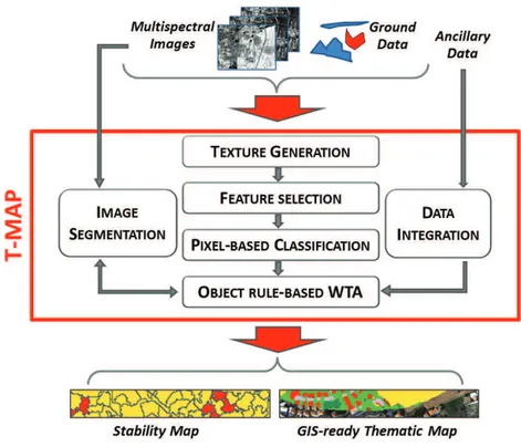
4.1 Overall workflow diagram describing the T-MAP approach with hybrid clas-sification. . . 40
List of Figures
4.2 Integration of elevation data. Left: study area. Center:
WorldView-2 RGB imagery. Right: LiDAR intensity. . . 41
4.3 Example of study area with permanent crops. . . 42
4.4 Workflow diagram describing the proposed hybrid classification schema with a priori integration. . . 43
4.5 Classification of study area using the radiometric WV2 dataset. 44 4.6 Overall Accuracy vs Number of Iterations for Training-Set and Control-Sets. . . 44
4.7 Accuracy through number of iterations. . . 45
4.8 Accuracy increases using LiDAR dataset for different classes and for bandsets. . . 46
4.9 Workflow diagram describing the proposed hybrid classification schema with a posteriori integration. (*) indicates possibility of adding LiDAR data to features space. . . 48
4.10 Pixel-based classification (left) and WTA classification (right) of the LiDAR data set. . . 51
4.11 GIS-ready CLC map and Stability map for the WV2+LiDAR classification. . . 52
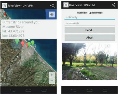
4.12 An example of Augmented reality application to monitor / send comments regarding an area of interest. . . 54
4.13 Architecture of the Whistland system. . . 56
4.14 Whistland database model for event and content management. 57 4.15 Mobile application in different operating states. . . 60
4.16 Merging and caching mechanism. . . 61
4.17 Geo-tweet heat-map. . . 63
4.18 Macro-area heat-map. . . 64
4.19 Animated geo-tweet heat-map. . . 65
4.20 System architecture with main components and exchanged data. 66 4.21 Indoor localization application. . . 67
4.22 RGB-D sensors system. . . 68
4.23 Fusion of Beacon and RGB-D position estimation. . . 68
4.24 Showroom floor plan with positioning framework. . . 69
4.25 Estimated distance comparison for different real distances. . . . 70
4.26 RSSI and distance relation. . . 71
4.27 Estimation error over time for different broadcasting power. . . 72
4.28 Error-map for “Beacons position estimation”. . . 73
4.29 Comparison of mean square error different position estimations. 74 4.30 Error-map for “Kalman position estimation”. . . . 74
4.31 Markov chain with a posteriori probabilities. . . 76
4.32 Heat-maps of paths. . . 77
List of Figures
4.34 Platform outline. . . 79
4.35 Induction loops. . . 80
4.36 Traffic acquisition devices. . . 80
4.37 Tracked bus with AVM system on map. . . 81
4.38 Video processing that count vehicles and individuates turns. . . 82
4.39 The identification process flowchart. . . 83
4.40 Example of foreground extraction: original frame (left), fore-ground image after MoG (middle), forefore-ground binary mask (right). Headlight reflections are circled in red. . . 84
4.41 Example of headlight removal: high value pixels from HSV (left), foreground binary mask without reflections (middle), final con-vex hull region (right). . . 84
4.42 The flowchart of the checkOldVehicles() function. . . 85
4.43 A partial vehicle-vehicle occlusion scenario. . . 86
4.44 A full vehicle-background occlusion scenario. . . 87
4.45 Data Analysis. Example of hourly capacity vehicles entering the city centre of Montemarciano in a typical working day. . . 89
4.46 Sample network with modifications. . . 90
4.47 Data Analysis. Example of hourly capacity vehicles increment-ing current recorded flows in a typical workincrement-ing day . . . 91
4.48 Felix robotic platform. . . 92
4.49 Felix system architecture. . . 93
4.50 Point Cloud visualization. . . 94
4.51 Virtual Reality compliance multi-view visualization. . . 95
4.52 Change detection visualization on point cloud. . . 96
List of Tables
3.1 Confusion matrix. . . 19
4.1 Difference Matrix on Minumum Overall Accuracy. . . 46
4.2 Difference Matrix on Minumum User Accuracy for Classes 110, 121, 122. . . 47
4.3 Difference Matrix on Minumum Producer Accuracy for Classes 110, 121, 122. . . 47
4.4 Acronyms related to the definition of rules. . . 49
4.5 Comparing different methodology by stability average value and standard deviation. . . 53
4.6 TweetPointer data structure. . . 58
4.7 Confusion matrix of classified “Kalman position estimation” per “area of interest”. . . 75
4.8 Path clustering results compared with range of ages. . . 77
4.9 Output sample of video processing. . . 82
4.10 Performance evaluation of the Profiles. . . 99
Chapter 1
Context
In this chapter we present the concept of next-generation geospatial applica-tions in the context of the evolution brought by Geomatics trends (Section 1.1). In Section 1.2 we outline the structure of the thesis.
1.1 Geospatial applications
Next-generation geospatial applications can be defined as applications using geospatial data that are not simple dots, lines and polygons, but complex ob-jects or evolution of phenomena that need advanced analysis and visualization techniques to be understood. This concept can enclose together many trends of Geomatics, such as low-cost sensors, free and open source software and HPC GeoBigData infrastructures.
To manage this kind of applications we need a data processing workflow that, in a semi-automatic way, brings raw data in something understandable to everyone, from the government to the citizen. In particular, this requires the analysis of geospatial data sources and platforms that can easily manage these data, including volunteered geographic information and crowd-sourcing geospatial data. For each geographical area, in most cases, there are different data that describe different aspect of phenomena. So we need to put together, integrate and combine these geo-data for the same area. The integration of multi-source data is a necessary challenging step to enrich description of phe-nomena in a geographical area. We are speaking about a phephe-nomena in a geographical area, so we expect to show data over the map. Visualization of raw-data, integrated-data, derivated-data with Web 2.0 technologies can be al-most everywhere and with any device. These emerging technologies are first of all the Cloud, to enable big data managing and processing on-demand with state-of-art Machine Learning and Deep Learning algorithm. Service oriented architecture, to define systems able to scale-up and grow with new implementa-tion. Interactive dashboard based on HTML5/JavaScript/CSS, to allow from every device with a web browser to look through the data.
Chapter 1 Context
While in the past mostly military interests dominated mapping activities, in the 20th century emphasis shifted to civilian/state organisations (i.e., National Mapping and Cadastre Agencies), mostly responsible for land administration, infrastructure planning or environmental monitoring. The mapping activity was carried out by trained staff based on well defined specifications, mapping and quality assurance procedures. It was only within the last years that a new player has entered the scene: the citizens themselves have started to become involved in mapping their environment. The development was made possible by progress in positioning and navigation, namely portable and low-cost GPS receivers often combined with a camera in a mobile or a smart phone, and in computer science, in particular the emergence of web 2.0 technology combined with broad band communication links. Most of the citizens lack formal training in mapping; furthermore map specifications and quality assurance procedures are often absent in these endeavours. Nevertheless, in many cases the quality of the resulting geo-spatial data is rather good. The borders between the previ-ously distinct roles of producer, service provider and user of geospatial data are substantially being blurred, as amateurs start doing the job of professional sur-veyors and distributors, and accomplish it rather well compared to traditional mapping products. The field is constantly growing and has lots of potential for mapping, mainly due to two reasons: the technology is mature and other ways to map may be too slow or too expensive. The term crowdsourcing is derived from outsourcing, where production is transferred to remote and po-tentially cheaper locations. Analogously, crowdsourcing describes the concept where potentially large user groups carry out work which is expensive and/or difficult to automate [1].
This rapid evolution and diffusion of technologies makes increasingly impor-tant the interconnection and the integration of different data-sources, with a greater attention to spatial dimension. Data fusion, as a general and popular multi-discipline approach [2], combines data from multiple sources to improve the potential values and interpretation performances of the source data, and to produce a high-quality visible representation of the data. Fusion techniques are useful for a variety of applications, ranging from object detection, recognition, identification and classification, to object tracking, change detection, decision making, etc. It has been successfully applied in the space and earth obser-vation domains, computer vision, medical image analysis and defence security, etc. Remote sensing data fusion, as one of the most commonly used techniques, aims to integrate the information acquired with different spatial and spectral resolutions from sensors mounted on satellites, air-crafts and ground platforms to produce fused data that contain more detailed information than each of the sources. Research on data fusion has a long history in the remote sensing community because fusion products are the basis for many applications.
Re-1.1 Geospatial applications searchers and practitioners have made great efforts to develop advanced fusion approaches and techniques to improve performance and accuracy. Fusing re-motely sensed data, especially multi-source data, however, remains challenging due to many causes, such as the various requirements, the complexity of the landscape, the temporal and spectral variations within the input data set and accurate data co-registration.
The process of visualization can reveal unexpected patterns and trends be-hind raw-data, making possible to interpret and express information as visual properties. Nowadays, the power of computation enables to map data with much larger datasets of thousands or millions of values, namely Geo-BigData platforms. Static visualizations are ideal when alternate views are neither needed nor desired, and required when publishing to a static medium, such as print, but are unable to represent well multidimensional datasets. The num-ber of dimensions of data is limited when all visual elements must be present on the same surface at the same time, so multiple static views are often needed to present a variety of perspectives on the same information. The views must be well designed to make the user effectively capable of understanding the information. The user is not able to analyse and view data from different points of view. Besides, different audiences need different perspectives, and these perspectives can change over time. Dynamic, interactive visualizations can empower user to navigate through the data for themselves [3]: overview first, zoom and filter, then details on-demand. This design pattern is found in most interactive visualization tools today [4] and is successful because it makes the data accessible to different audiences, both new to the subject matter or already deeply familiar with the data. An interactive visualization that offers an overview of the data alongside tools for ”drilling down” into the details may successfully fulfil many roles at once, from those who are merely browsing or exploring the dataset to those who approach the visualization with a specific question in search of an answer. The best way to make available analysis and visualization tools is the publication on the web. Working with web-standard technologies (HTML, CSS, JavaScript, SVG) allows geospatial data to be seen and experienced by anyone using a recent web browser, regardless of the op-erating system (Windows, Mac, Linux, Android, iOS) or device type (laptop, desktop, smartphone, tablet). Moreover, many web-standard technologies are open source and usable with freely accessible tools. This opens to innovative contributions from the web community. Researchers and practitioners are still working to continuously improve user experience, communication efficacy and interoperability, following the evolution of new devices, technologies and data.
Chapter 1 Context
1.2 Structure of the thesis
The thesis is organized as follows. Chapter 2 presents state-of-the-art in manag-ing, integrating and visualising geospatial data sources. In Chapter 3 the overall workflow is presented, delineating main steps from raw-data to final presenta-tion. Chapter 4 describes some developed geospatial applications, focusing the attention on the implementation of the presented workflow to combine multi-source data. Finally, Chapter 5 outlines conclusions and future works.
Chapter 2
State of art
In this chapter we introduce different geospatial data sources used in our work (Section 2.1). In Section 2.2 we present the state of art for integration of multi-source data, while in Section 2.3 for visualization based on technologies of Web 2.0.
2.1 Geospatial data sources
Emerging concepts as Wireless Sensor Networks (WSN), Internet of Things (IoT), social networks (i.e., Twitter, Instagram, Facebook) and crowd-mapping (CM) are combined and mixed to develop novel and user-oriented applications that bring higher value information to companies and researchers. These tech-nologies have increased the number of available geo-data sources contributing to open mapping to everybody, not only government authorities. Data can be (and have been) donated to open projects, mainly from government authorities; from raw GPS tracks and images to fully labelled vector data.
Many social networks today contribute to the emergent Geospatial Web [5] by implementing the geo-tagging of content (text, audio, images/videos) in their Application Program Interfaces (APIs) for mobile applications. The ge-olocation of published contents on social networks allows the development of systems able to detect in real-time trends of any type. The spatial-temporal analysis of social media trends for abnormal event detection, supported by lan-guage identification and analysis [6, 7, 8, 9, 10], allows identifying in short time events of interest in a given region.
In the last years, the IoT phenomenon induced a lot of interest on industries and research groups [11, 12], with applications ranging from home monitor-ing [13] to precision agriculture [14]. Recent works exploited the use of WSN for disaster management [15, 16], enhancing the context awareness with perva-sive and continuous raw information.
The combination of automatically acquired raw sensor data and social trig-gered information could be disruptive for the users of geospatial applications. Nowadays, this potentiality is exploited for commercial purposes, like in Google
Chapter 2 State of art
Maps when you are invited to publish a post to social media after a place visiting detected by your mobile GPS or by IoT devices [17] (i.e., Bluetooth iBeacons). Anonymized signals of mobile phones carried by car drivers or pedes-trians are being used to map out roads or pedestrian walkways [18], without people being aware of it [19].
The term crowdsourcing is commonly used to describe data acquisition us-ing web technology by large and diverse groups of people [20]. In many cases these people do not have particular computer knowledge and are not trained surveyors [21]. Then, these acquired data are transferred to and stored in a common computer architecture (e.g. a central or a federated database) or in a cloud computing environment [22]. The subsequent tasks of automatic data integration and processing are very important to generate further information from the acquired data, sometimes also in feedback loops with data acquisition, and provide multiple research challenges [23]. In a flooding event occurred in Genoa (Italy) on October 2014, the OpenGenova system has been developed to map crisis area by using (geo)photos and hashtag on the Instagram social network, even if not in real-time [24]. Since the earthquake of Haiti in Jan-uary 2010 [25], the crisismappers established a new concept of cooperation to increase the knowledge of territory, exploiting satellite/aerial maps and city models/road graphs [26, 27, 28]. In next-generation geospatial applications traditional geo-data (i.e., satellite/aerial images) have been augmented/inte-grated/updated with ground images from mobile phones, mobile mapping vans and from UASs (unmanned aircraft systems). These three platforms are in-teresting, because in this way users can acquire their own images of a local neighbourhood and thus do not have to rely on images available on the web. Image orientation is determined fully automatically to avoid pitfalls [29] thanks to GPS receiver equipped on these platforms that further constraining the so-lution. The main advantage of using ground acquired images is the quasi real-time update (satellite/aerial images are subject to scheduling, cloud coverage) and a high-resolution view of the area [30]. It is well known from traditional mapping that operators familiar with the local environment make less errors during data acquisition, have fewer problems in dealing with ambiguities and thus derive higher quality results. Crowdsourcers are often most interested to map their immediate surroundings, which is the area they know best.
In the last few decades traditional data gathering methods ranging from field survey to conventional photo-interpretation of aerial photographs were used for mapping purpose and then portrayed on a map using standard carto-graphic methods. However, technical advances in the last three decades have completely changed the picture. Nowadays the availability of high spatial res-olution imagery from satellite sensors (IKONOS, Quickbird, Worldview, . . . ) and digital aerial platforms (Leica ADS40/80 and following series, Vexcel
cam-2.1 Geospatial data sources era,. . . ) provides new opportunities for detailed territory mapping at very fine scales, in particular if combined with modern technologies for Light Detection And Ranging (LiDAR) data acquisition. Higher resolution sensors for spectral data (increasing also the radio dynamics), and increased measurement-point density [31]. Moreover, the time-resolution of acquisition can be strongly re-duced installing sensors on innovative vehicles as Unmanned Aerial Vehicles (UAVs) for civilian [32] or military applications [33] breaking down the cost of data for square kilometre.
Figure 2.1:Satellite imagery and LiDAR intensity data.
Several authors have combined high resolution multispectral and LiDAR data. LiDAR data provide important position and height information, while the high-resolution multispectral imagery offers very detailed information on objects, such as spectral signature, texture, shape, etc.. A sample of these two datasets is presented in Figure 2.1. Zeng et al. (2002) [34] show an improvement in the classification of IKONOS imagery when integrated with LiDAR, Syed et al. (2005) [35] underline how this integration makes the object-oriented classifi-cation superior to maximum likelihood in terms of reducing “salt and pepper”. Ali et al. (2008) [36] describe an automated procedure for identifying forest species improved by high-resolution imagery and LiDAR data. The integration of multispectral imagery and multireturn LiDAR for estimating attributes of trees is reported in Collins et al. (2004) [37]. Alonso and Malpica (2008) [38] combine LiDAR elevation data and SPOT5 multispectral data for the classifi-cation of urban areas using a Support Vector Machine (SVM) algorithm. Ke et al. (2010) [39] combine QuickBird imagery with LiDAR data for object-based classification of forest species. Forest characterization using LiDAR data is dominated by high-posting-density LiDAR data (Reitberger et al., 2008 [40]) due to the ability to derive individual tree structure. Low-posting-density
Li-Chapter 2 State of art
DAR data, although less costly, have been largely limited to applications of terrestrial topographic mapping (Hodgson and Bresnahan, 2004 [41]). Wang et al. (2012) [42] combine QuickBird imagery with LiDAR-derived metrics for an object-based classification of vegetation, roads and buildings.
Combining these two kinds of complementary datasets is shown to be quite promising also for building detection (Rottensteiner et al., 2003 [43]; Khoshel-ham et al., 2010 [44]; Tan and Wang, 2011 [45]), road extraction (Hu et al., 2004 [46]; Azizi et al., 2014 [47]; Hu et al., 2014 [48]), 3D city modelling (Awrangjeb et al., 2013 [49]; Kawata and Koizumi, 2014 [50]), classification of coastal areas (Lee and Shan, 2003 [51]), evaluation of urban green volume (Bork and Su, 2007 [52]; Zhang et al., 2009 [53]; Tan and Steve, 2011 [54]; Huang et al., 2013 [55]; Parent et al., 2015 [56]) and for a better characteriza-tion of the surveyed scene in general.
Recent research by Germaine and Hung (2011) [57] delineate impervious surfaces from multispectral imagery and LiDAR data by a knowledge based expert system Rodriguez-Cuenca et al., 2014 [58] conduct an impervious / non-impervious surface classification using a decision tree procedure.
2.2 Integration of multi-source data
Pohl and van Genderen, 1998 [59] classified remote sensing fusion techniques into three different level, according to the stage at which the fusion takes place (see Figure 2.2): the pixel/data level, the feature level and the decision level. Often, the applied fusion procedure is a combination of these three levels, since input and output of data fusion may be different at different levels of processing. Fused images/data may provide increased interpretation capabilities and more reliable results since data with different characteristics are combined.
Pixel level fusion is the combination of raw data from multiple sources into single resolution data which are expected to be more informative and synthetic than either of the input data or reveal the changes between data sets acquired at different times [60, 61, 62].
Feature level fusion extracts various features (e.g. edges, corners, lines, tex-ture parameters, etc.) from different data sources and then combines them into one or more feature maps that may be used instead of the original data for further processing [63, 64]. This is particularly important when the number of available spectral bands becomes so large that it is impossible to analyse each band separately. Methods applied to extract features usually depend on the characteristics of the individual source data, and therefore may be differ-ent if the data sets used are heterogeneous. Typically, in image processing, such fusion requires a precise (pixel-level) registration of the available images. Feature maps thus obtained are then used as input to pre-processing for image
2.3 Visualization
Figure 2.2: Processing levels of image.
segmentation or change detection.
Decision level fusion combines the results from multiple algorithms to yield a final fused decision [65, 66]. When the results from different algorithms are expressed as confidences (or scores) rather than decisions, it is called soft fusion; otherwise, it is called hard fusion. Methods of decision fusion include voting methods, statistical methods and fuzzy logic based methods.
2.3 Visualization
The use of the Internet to deliver geographic information and maps is burgeon-ing, in the last decade we are speaking of th GeoWeb [67]: map mash-ups, crowdsourcing, mapping application programming interfaces (API), neogeog-raphy, geostack, tags, geotechnologies and folksonomies. These rapid devel-opments in Web mapping and geographic information use are enabled and facilitated by global trends in the way individuals and communities are us-ing the Internet and new technologies (Web 2.0 [68]) to create, develop, share and use information (including geographic information), through innovative, often collaborative, applications. The impacts of Web 2.0 can be considered in terms of the underpinning technologies and the characteristics of application development and use they enable. While initial popular use of the Web was characterised by websites that enabled the distribution of information in new
Chapter 2 State of art
ways but with a limited interaction, the technologies of Web 2.0 provide a far richer user interaction and experience. Several factors have provided a plat-form for these new applications. First, a massive data transfer capacity became available at very low costs, enabling the proliferation of broadband services to home users. Second, technology companies developed standards that allowed the transfer of information between distributed systems in different locations. This family of standards (including OGC standards [69] and GPX [70]) were based on XML. Another innovation, which integrates XML-based standards and allows the development of sophisticated applications, is the AJAX (Asyn-chronous JavaScript and XML). As Zucker, 2007 [71] notes, the most important innovation in AJAX is in the ability to fetch information from a remote server in anticipation of the user’s action and provide interaction without the need to refresh the whole Web page. This changes the user experience dramatically and makes the Web application more similar to a desktop application where the interaction mode is smooth. AJAX-based geographical applications look and feel very different. First, the area of the screen that is served by the map has increased dramatically, thus improving the usability of Web mapping sig-nificantly. Second, the ability to interact within the browser’s window changed the mode from the ”click-and-wait-for-a-page-refresh” to direct manipulation of the map – a mode of interaction familiar in other desktop applications, and more akin to desktop GIS.
The modern Web 2.0 platforms are build over a backend for easily creat-ing and managcreat-ing services and applications for both mobile clients and Web browsers. Taking care much of the complexity at the backend infrastructure side, the creation of applications on top of this service platform is faster, sim-pler and open also to 3rd parties developments. REST [72] is the more common architectural style for these platforms.
Large virtual 3D scenes are essential to systems, applications, and technolo-gies. In general, these models represent a complex artifact or environment and allow users to visualize, explore, analyze, edit, and manage its components (i.e., they serve as tools to effectively communicate spatial information). With the rapidly growing demand for web-based and mobile applications, it becomes crucial for system and application developers to provide web-based, interactive access to large, virtual 3D scenes [73, 74]. In this challenging field researchers try to realize as much as possible a server-client communication that is inde-pendent from the 3D scene complexity and supporting interactive and robust 3D visualization on the clients [75].
At the same time, AR is a promising and continuously evolving technol-ogy [76] that is actually applied in many contexts as cultural heritage [77, 78], education [79], shopping [80], geographic visualization [81, 82, 83], environ-mental monitoring [84] and also to disaster management [85]. The capability
2.3 Visualization
Figure 2.3: 3D model visualization.
to see in real-time virtual objects overlying images captured from cameras aug-ments the experience of a user that can view and explore more contents, as in Figure 2.4, often gathered from the web (i.e., multimedia related content or georeferenced information).
Because CM [22, 21, 23] starts from geo-data (satellite/aerial imagery) that are not easy to understand by common people, the capability of considering together CM and AR systems plays a key role, in particular, for a rational management of natural disasters [86].
Chapter 2 State of art
Chapter 3
Materials and methods
In this chapter we present (Section 3.1) the processing workflow designed in geo-spatial applications starting from geo-data sources. In Section 3.2 we de-scribe in detail processing techniques implemented to extract information from raw-data. In Section 3.3 we present visualization technologies, from Web 2.0, exploited to show information to final users.
3.1 Workflow
The objective of the designed workflow, outlined in Figure 3.1, is to bring raw data in something viewable and understandable to everyone. The platform that should acquire geo-data sources can be represented with different data-model, managed by geo-spatial applications:
• Image/Raster - digital aerial photographs, imagery from satellites, digital pictures or even scanned maps;
• Video - moving visual media recorded by high-resolution video cameras with improved dynamic range and color gamuts;
• Data/Vector - other geo-data that provide a way to represent real world features, in general associated with a geometry (point, line, polygon, . . . ); Nowadays, these data are generated through other channels, not dedicated to survey or mapping activities:
• Sensor - information collected by IoT smart devices, both passively, by performing sensing operations, and/or actively, by performing actions; • Mobile - digital footprints collected by mobile devices;
• Social - user-generated content, such as text posts or comments, digital photos or videos, and data generated through all online interactions.
Chapter 3 Materials and methods
Figure 3.1: General Workflow.
These geo-data sources can aliment applications in real-time with a direct connection (i.e., Bluetooth, Wi-fi, . . . ) or indirect connection through a Cloud platform. In general we need an interface to read these data and realize an abstraction layer to elaborate them. In some cases the interface is already pro-vided with an HTTP server over an IP protocol, in other it must be developed based on current data-types and processing pipelines. Each method used in this general workflow can be categorized in the following five classes:
3.1 Workflow definition of regions of interest within a scene;
• Classification - starting from a training set, to identify to which category new data belong;
• Change Detection - to compare data of the same phenomena to detect whether or not a change has occurred or whether several changes might have occurred and eventually to signal anomaly detection;
• Tracking and Path Clustering - objects or users are tracked through time and their path or trajectory can be aggregated in similar groups;
• Simulation and Prediction - data are first used to build a simulation/pre-diction model and then, after a validation step, to simulate real/new conditions or to predict an evolution of phenomena observed.
Each method is often composed of a series of different steps, typical for every reference domain. Outputs of a processing block are elaborated/fused/derived data that are structured to be ready for being published on visualization plat-forms, displayed on a web page linked to a database. These platforms are mostly Web-based and are optimized also for mobile devices. Back-end data services that expose information to front-end clients use RESTful interface, with JSON or XML as exchange formats. When the data are in binary for-mat, such as images, meta-data and descriptors are often represented in these exchange formats. The visualization technologies used in this general workflow are:
• Web/Map Dashboard - provides at-a-glance views of KPIs (key perfor-mance indicators) relevant to a particular objective, using maps to rep-resent spatial distribution and evolution of a phenomena;
• 3D Point Cloud - provides a visualization tool to view complex 3D models and point clouds, adaptable and scalable for fluid rendering with different devices and bandwidths;
• 360◦Image and Video - provides an immersive experience inside a virtual
reconstruction of a real environment;
• Augmented Reality - provides a live direct or indirect view of a physical, real-world environment whose elements are recognized and ”augmented” with additional information or contextual contents.
Chapter 3 Materials and methods
3.2 Processing
3.2.1 Segmentation and Identification
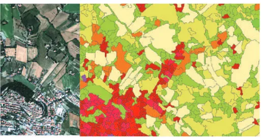
Segmentation of digital image is the process that determines multiple segments (sets of pixels, also known as super-pixels), also called regions, partitions, or objects.
Figure 3.2: Image segmentation.
For image segmentation many different algorithms have been used, which divide the image into regions with common characteristics based on key fea-tures extracted from the dataset (e.g., geometrical or spectral/colorimetric). In general the approach is based on a region growing algorithm, where the adjacent pixels are grouped in the same region by spectral similarity assur-ing some shape parameters (i.e., compactness, convexity, etc.). Figure 3.2 shows the input satellite imagery and the image segmentation obtained from a specific-developed region growing algorithm. Specific algorithms can differ by the way of choosing initial pixel for growing procedure or in the number and kind of spectral/geometrical parameters and their weights. The idea is to obtain meaningful objects able to better represent information in the image, directly understandable by humans. Sometimes the algorithm try to reproduce the knowledge process of a human to replicate the same representation, in other cases extract information not recognizable by “naked eye”.
Second and necessary step in this process is the identification of “regions of interest”. The segmentation algorithm divides a digital image in multiple segments, then objects can be identified on the basis of key characteristics (e.g., geometrical or spectral/colorimetric). Some smaller or irregular regions are ignored or merged with greater ones, while for identified regions a refinement
3.2 Processing process can be applied to increase segmentation quality. Using satellite/aerial imagery, this second step can be driven by ancillary data, coming from other sources such as official maps, previous surveys or crowd-source information.
Figure 3.3: Video foreground extraction.
With respect to still images, working with video frames requires algorithms that identify moving objects, more in general which regions are changed frame by frame. Mixture of Gaussians (MoG) background subtraction can be success-fully used to extract foreground pixels, given them as input to a segmentation step that identifies regions and finally performs moving object detection. Fig-ure 3.3 and FigFig-ure 3.4 show a sequence of images, from left to right, represent-ing extraction and refinement processes which start from the object identified, highlighted by a blue rectangle, and ends with a more precise contour, remov-ing headlight reflections circled in red. The complete algorithm is presented in Subsection 4.4.2.
Figure 3.4: Video foreground refinement.
The input of a segmentation/identification algorithm is a digital image or a video frame and the output is a vector with contours of identified objects. In general this is a first result in the processing workflow and these objects are usually the starting point for a classification algorithm or a tracking process.
Chapter 3 Materials and methods
3.2.2 Classification
Automatic classification has been carried out according to two approaches: a pixel-based and an object-based method. Pixel-based classification aims at identifying the classes by means of the spectral information provided by each pixel belonging to the original image bands. The object-based approach oper-ates on sets of pixels (objects/regions) grouped together by means of an image segmentation technique.
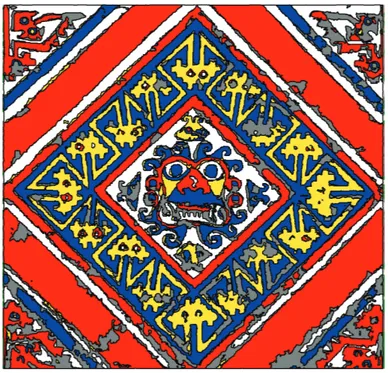
Figure 3.5: Training data set.
To perform a supervised classification we need to provide a training data set referred to different classes. In Figure 3.5, the training samples are defined for each pigment in the five classes: red, white, yellow, blue and gray. The Maximum Likelihood algorithm is the simplest approach to obtain an image classification, but many other algorithms can be applied with different results in term of accuracy. The result of the pixel classification is an image with most of pixels assigned to a class and others left undefined, Figure 3.6.
To assess the quality of the training process we need to compare assigned value (Predicted class) by the classificator against the sample regions (Ground Truth). Moreover the same operation must be done for other regions, called test dataset, to assess the quality of the classification process. The assessment is summarized in a confusion matrix, Table 3.1, which is a simple tool to understand overall/per-class accuracy and reliability. The right classified pixels are on the table diagonal, while other values represent misclassified pixels.
3.2 Processing
Figure 3.6: Pixel classification.
Table 3.1: Confusion matrix.
Ground/ 1 2 3 4 5
Predicted red white yellow blue gray Accuracy
1 - red 3.704 0 46 0 222 93.25% 2 - white 0 4.212 0 0 115 97.34% 3 - yellow 0 2 3.843 0 5 99.82% 4 - blue 0 0 0 2.988 2 99.93% 5 - gray 0 80 0 94 1.115 86.50% Reliability 100.00% 98.09% 98.82% 96.95% 76.42% 96.55%
Overall/per-class accuracy and reliability can be improved adding other in-formation, such as elevation. Before and after a classification step the data can be submitted to a pre- or post- processing phase. For digital image, various image filtering or enhancing techniques can be applied to reduce the noise of the sparse pixels, such as a salt and pepper filter, and to compensate other issues due to acquisition sensor characteristics or to combine other information from heterogeneous sources.
A pixel based classification is a typical process on digital image, which for geo-spatial applications are commonly named raster data. In many cases this is not enough for advanced applications: a group of similar pixels must be considered as an object, for example a footprint of an industrial building
con-Chapter 3 Materials and methods
nected with a plant/function and belonging to a company. Vector model can be a more convenient way to represent geo-spatial information, in particular to manage more information in a GIS.
Figure 3.7: Object classification.
An object-based classification method starts from the output of a segmen-tation process and assigns a class to each segment, Figure 3.7. In general the classification works on a subgroup of features, extracted or generated for each region in a first step called “Feature Extraction” and selected in a second step called “Feature Selection”. The object-based classification improves the result in terms of spatial consistency, semantic representation and GIS ready production, more comprehensible for the end user.
All the extracted features become attributes of each object with the possi-bility to implement a rule-based system and to include the pixel-based clas-sification result, by the Winner-Takes-All (WTA) approach [87], in a hybrid classification algorithm 3.8. For each segment counting pixels belonging to each class, the area percentages and the predominance per region of the most frequent class, the winner, are determined. According to this methodology a stability map is generated, by considering, for each segment, the ratio between the second-best and the winner class for each segment. Areas with stability indices close to one unity have to be reviewed while others are to be considered reliable.
3.2 Processing
Figure 3.8: Hybrid classification.
More complex approaches to extract features and classify images can be taken from Deep Learning techniques, such as Deep Convolutional Neural Net-works (DCNNs). In satellite/aerial imagery, which is constituted of complex scenes, input of a neural network can be small parts of a scene, objects identi-fied from a previous segmentation algorithm that represent different pictures. The classification objective can be different from defining the pixel or object class of each identifiable element inside the picture, and can be a categoriza-tion of the picture as a whole. We need a more general approach, because pictures coming from other sources (i.e., cameras, mobile devices and social media) can contain overlying textual information that could influence classifi-cation result, in particular the sentiment/polarity connected to the image (e.g., positive, neutral, negative). We need a joint visual and textual analysis: a vi-sual feature extractor, a textual feature extractor and a fusion classifier. The visual feature extractor provides information about the visual part of a pic-ture and is therefore trained with image labels indicating the visual category of the images, as a common image classification. The textual feature extractor is divided into sequential step: (i) detection of individual text boxes, (ii) ar-rangement to form logical lines based on a left-to-right or top-to-bottom policy
Chapter 3 Materials and methods
(iii) optical text recognition and (iv) encoding based on the alphabet of the character-level DCNN. On the basis of the visual and textual features, a fusion classifier estimates the overall content of an image [88]. The performance of the classification is always evaluated with precision and recall, overall and for each category.
3.2.3 Change Detection
A change detection approach compares data of the same phenomena, detecting whether or not a change has occurred, or whether several changes might have occurred, and eventually signalling an anomaly detection. A change detection method should automatically find the changes in the studied area and update the corresponding map, model or database accordingly. In satellite/aerial im-agery and in general pictures, a first approach to identify changes between two ´epoques can be a raster pixel by pixel difference operation, Figure 3.9. To make images spatially comparable, first we need a transformation to align im-ages among control points and a re-sampling to have the same pixel size [89]. To make images spectrally comparable we need a pre-processing to correct gamma colour, contrast and other characteristics.
Figure 3.9: Change detection by pixel.
This first change detection approach is affected from noise in raw data and needs a post-processing to refine results, reducing sparse changes and
evidenc-3.2 Processing ing greater ones. Another technique that doesn’t need a pre-processing to make images spectrally comparable uses classified values. Pixels are not compared with their spectral values, in a common picture red-green-blue, but with their classes. This approach can produce better result, according to precision and reliability of the applied classification method.
From pixel-based change detection we can move forward to object-based change detection, Figure 3.10, where the comparison is made on homologue regions obtained from a segmentation process. To be spatially consistent, the comparison can be done on a segmentation produced with the intersection of two original segmentations. With more than two images this approach cannot be feasible, so it is more convenient to establish a reference epoch with its objects and try to identify their evolutions.
Figure 3.10: Change detection by object.
To detect visual changes from the photos, we can apply state-of-art classifiers, such as k-Nearest Neighbors (kNN) [90], Support Vector Machine (SVM) [91], Decision Tree (DT) [92] and Random Forest (RF) [93]. The classification process is carried out with the aim to automatically detect anomalies: deep learning methods can be used to classify different classes of anomalies with an opportune training on labelled images.
Not only images are used for change detection by applying image differencing and also point clouds can be used to detect changes in a similar way. Change
Chapter 3 Materials and methods
detection can be done in several ways: by the comparison of raw point clouds, coloured point clouds, voxels, range images, surface models or modelled objects. The common way to compare two point clouds is to measure distances between points in different point clouds and evaluate if a point in one point cloud has neighbours nearby in the other point cloud, otherwise the point is marked as a potential change. Adding the average colour of images into the point clouds provides additional information about the possible changes. Point clouds can be also converted into 3D surfaces. Changes can also be detected using object models. If the point cloud can be modelled into separate classified objects, it can be checked if the objects can be found in both point clouds.
Point wise distances of two point clouds can be calculated as:
d(p1, p2) =p(x1−x2)2+ (y1−y2)2+ (z1−z2)2 (3.1)
where p1 is the first point with coordinates (x1, y1, z1) and p2 is the second
point with coordinates (x2, y2, z2).
Every generated point cloud is associated with a specific segment that is uniquely identified in the infrastructure network. This is necessary to correctly manage S&C (safety & crossing) and trace variation over time.
Figure 3.11: Change detection on point cloud.
To automatically highlight these variations, it is used CloudCompare [94], an open source software, as shown in Figure 3.11. Red points have greater distance from the original point cloud and represent changes. This tool allows to compute signed distances on a point cloud rather than on a meshed surface.
3.2 Processing
3.2.4 Tracking and Path Clustering
A robust tracking is essential to monitor objects that are moving in the space, both indoor and outdoor. Instant positions can come from a positioning system, like GPS in a mobile device, or other localization systems (i.e., Bluetooth, Wireless, Radio, or mixed systems). Using a multi-sensor system that fuses different data can reach a better position estimation and can overcome some issues of coverage, disturbance and precision [95, 96]. The accuracy evaluation of positioning systems is based on measurement of errors in ground-points with well determined position, Figure 3.12.
F E D C B A 9 8 7 6 5 4 3 2 1 20 19 18 17 16 15 14 13 12 11 10 B1 B4 B5 B6 B3 B2 SRC RGB-D ³ ³ ³ ³ ³ ³ Error (m) 5 4 3 2 1 0 Ground-point
Figure 3.12: Error-map for position estimation in indoor environment. In these cases the moving object is already identified by a device address or identification code and the most precise position with the lowest sensor cost and size/weight is desirable.
In other situations, like in video surveillance, the object must be previously segmented and identified, so information must be gathered frame by frame during the object lifetime in the scene [97]. Moreover in multi-camera systems the same object must be recognized not only frame by frame, but also from a camera to another [98]. The challenge is to design a robust tracking system that is able to manage occlusions in the scene, without the loss of object’s identity. For example in vehicle surveillance, vehicles are occluded each other, Figure 3.13, or vehicles are behind background objects, Figure 3.14. A robust algorithm must be able to correctly re-identify tracked objects after occlusion periods.
Chapter 3 Materials and methods
Figure 3.13: Vehicle-vehicle occlusion scenario.
Figure 3.14: Vehicle-background occlusion scenario.
if the object is moving and in which direction. In many applications, in a retail environment or in a museum or in general in a space, it is very interesting to know how many people are standing in a particular area and for how much time. This can be represented as an heat-map with a density summarizing the number of people over time or the permanence time periods, Figure 3.15.
Secondly, we can determine the movement as a path made of discrete po-sitions. This non continuous sequence depends on the frequency of position estimation, usually 1 per second in a GPS device, and on the precision, usually in the order of meters for navigation. If we had a pre-determined fixed path it is simpler to identify the position along it. Moreover, if we do not want a precise trajectory or simply we cannot have it, we can determine the path as a sequence of visited areas. In particular, points falling into the transition buffer between areas can be classified into different “area of interest”, showing in the movement path an apparent “returning-back” or “chattering” effect, although the subject was moving straight to the other area. To correctly reconstruct the subject paths and overcome this issue, we can introduce a temporal filter, ignoring passages lasting less than a duration threshold or too far from the pre-dicted position. In many cases this sequence of “area of interest” is sufficient
3.2 Processing F E D C B A B1 B4 B5 B6 B3 B2 SRC RGB-D
Figure 3.15: Heat-maps of tracked people.
for a coarse analysis of the behaviour of people that are moving in the spaces. After this path reconstruction it is clear that other elaborations can be done. We can compute presence probability for each “area of interest” and transition probability for every passage between adjacent areas, constructing a Markov chain with a posteriori probabilities Figure 3.16.
A
B
C
D
E
F
63% 22% 38% 55% 35% 14% 15% 7% 10% 21% 14% 14% 0% 2% 18% 45% 35% 21% 76% 48% 6% 41% 25% 20% 17% 10% 9% 19%Figure 3.16: Markov chain with presence and transition probabilities. These probabilities can be used to analyse movement trends inside the space and compared with a priori expected behaviour can provide indications to
Chapter 3 Materials and methods
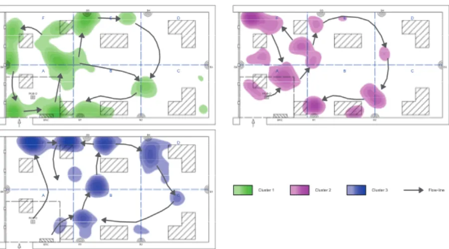
improve the visiting experience in a retail environment or in a museum. We can proceed with a path clustering, using for example Expectation Max-imization (EM) [99], to point out correspondences that should exist between recorded paths and other information, such as user profiles in Figure 3.17. We can show these correspondences with heat-maps and flows: darker colours rep-resent a longer permanence time and arrows are a schematic reprep-resentation of flow analysis. F E D C B A B1 B4 B5 B6 B3 B2 SRC RGB-D F E D C B A B1 B4 B5 B6 B3 B2 SRC RGB-D F E D C B A B1 B4 B5 B6 B3 B2 SRC RGB-D Cluster 3 Cluster 2 Cluster 1 Flow-line
Figure 3.17: Heat-maps of paths computed by cluster.
3.2.5 Simulation and Prediction
Previously presented techniques are devoted to analysis purposes: data are fused/combined/processed to extract information that are significant to un-derstand an aspect of the reality. These data can be also used to build and feed a simulative or predictive model: we want to know where we are now, simulating where we can go or predicting where we will go.
Simulation, in the ambit of Intelligent Transportation System, is very use-ful to increase planning quality of an infrastructure. The complexity of the simulation problem induces to build a traffic model choosing an existing sim-ulator/platform, such as SUMO (Simulation of Urban MObility) [100]. The simulation platform must be customizable to manage particular situations and able to handle large road networks. The main design criteria to follow in this choice are:
• Portability: simulation has to run on any common environment, since many research organizations use Linux or Solaris as operating system. • Extensibility: simulation has to be open and easy to understand, so that
3.2 Processing
Figure 3.18: Road network.
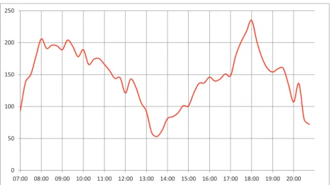
0 50 100 150 200 250 07:00 08:00 09:00 10:00 11:00 12:00 13:00 14:00 15:00 16:00 17:00 18:00 19:00 20:00
Figure 3.19: Traffic demand.
The SUMO simulation platform represents the road network infrastructure, Figure 3.18, and the traffic demand, vehicles flow as hourly capacity in Fig-ure 3.19, and it can be used in different research problems: route choice, traffic light algorithms, simulating vehicular communication and many others [101]. The traffic model can be feed with raw-data acquired by sensors or using his-torical data to estimate the conditions in different periods. Multi-source data can be integrated in a consistent and validated model useful to reconstruct the actual traffic and able to simulate different traffic conditions (i.e., inten-sive summer flows generated from seaside, especially in the weekend). We can
Chapter 3 Materials and methods
simulate future traffic situations against road network to highlight the critical points and develop right solutions. We have introduced possible variations to roads according to analysis of simulation results. Low cost modifications, like the change of direction of travel for some one-direction streets, medium cost, like variation of a cross with the realization of a lane of accumulation, high cost, like the substitution of a traffic light with a roundabout. The simulation platform allows a technician to show this data and interact with the traffic model and the simulator.
Simulation results and models can be useful also for prediction applications. This is a challenge, in particular in the ambit of Industry 4.0, where the sensorization of production and the transformation of products in IoT nodes generate a large amount of data along the value chain from supplier to con-sumer [102]. A predictive model can help in the phase of control production an-ticipating problems and malfunctions, consequently reducing production waste and machine stops. Moreover, can improve significantly the customer service, optimizing product for customer needs and anticipating problems and malfunc-tions.
Figure 3.20: Predictive maintenance snapshot.
In general, data sent from the IoT nodes are stored in the cloud server. The cloud platform provides all the tools to manage Big-Data and a framework to quickly develop applications and interfaces for smart-phones and computers. The data collected and properly organized allow to apply machine learning al-gorithms to analyse the history of the activities carried out by the device and to
3.3 Visualization predict possible malfunctions. Therefore, it can be carry out a preventive main-tenance through alert mechanisms, for example on decay of the performance in time. In Figure 3.20, the blue line represents the standard degradation that provides for a change of component after about 12 months of use (with a twice daily use). The orange line represents an example of degradation calculated on historical data for the device; in this case the component change can be delayed compared to the standard.
3.3 Visualization
3.3.1 Web/Map dashboard
To better understand the geographical area involved in an event or to know and analyse all the events that have affected a specific region, a web dash-board is the more flexible and usable tool to reach the goal. In general, the dashboard is built with a responsive template engine, such as Bootstrap (www.getbootstrap.com), allowing to develop once and run on almost every device.
A thin JavaScript client can be implemented exploiting the RESTful API exposed by a back-end server: the server returns information (mainly in JSON or in XML), so the client is responsible for further processing and for rendering. In this way, the server is not overloaded by unnecessary operations (i.e., pro-cessing and rendering) and the load is distributed among all the clients. The dashboard can generate reports for events, regions or their combinations with synthetic indicators, tabular reports, graphs and heat-maps.
Dashboard are dynamically rendered on the basis of the data retrieved by the filters specified by the user through the interface. An heat-map represents distribution of the geo-localized data involved in a specified event. For example in Figure 3.22 more intense green indicates higher density, while red represents the maximum concentration. The geographical regions are organizable in a hierarchy to allow analysis with different levels of spatial aggregation.
Graphs and heat-maps can be animated slicing all the data in time windows, adopting the technique described in [103]. Each window has a start and an end date and contains all the data published within this interval. The timing engine acts as a player for the graph, retrieving all the data inside each window: com-paring this process to a media player, each window corresponds to a “frame”. User specifies temporal bounds of the analysis and the length of the window. The dashboard loads all the event data inside specified temporal bounds and slices the tweets, according to window’s length. Moreover, user can adjust the rate of the playback, specifying the duration of each frame. This mechanism allows the user to understand the dynamic of an event, taking into account also
Chapter 3 Materials and methods
Figure 3.21: Dashboard with Interactive heat-map, table and graph.
Figure 3.22: Animated heat-map.
the temporal dimension alongside the capability to perform spatial queries, as shown in Figure 3.22.
To increase user analysis capabilities, the dashboard allows overlaying, as layer on the maps, all georeferenced data stored in the back-end. The web-GIS viewer can also visualize other sources of geo-data published on Internet, which are supported by the JS library used to develop it. This feature is very important when there is the necessity to integrate and visualize ancillary data trusted by a government source.
3.3 Visualization
3.3.2 3D Point Cloud
In many survey contests, for example buildings, a fast acquisition is done, for example by laser, which allows obtaining x, y, and z coordinates for each surveyed point. Using a camera, spectral information can be acquired and, after a correct co-registration between these two dataset, also the “colour” information can be added. This type of acquisition generates a great amount of raw-data that must be processed to obtain an useful reconstruction as a manageable 3D model. Moreover, the web visualization becomes a challenge due to the quantity of data to transmit and render in an usable interface. The generated point data must be converted in a tree structure, for example using the PotreeConverter tool [104]. This tool is usually employed to convert an input coordinate files to the required point cloud data structure that is optimized for visualization at different levels of detail. The data structure in output can be easily visualised on a web platform based on Potree, a viewer for a large point cloud/LIDAR datasets (Figure 3.23).
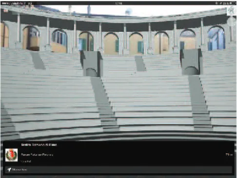
Figure 3.23: Point Cloud Viewer.
The web viewer can provide, to almost every device with a browser, mea-surement tools, layer overlaying, filter tools and animation capabilities.
3.3.3 360
◦Image and Video
With the expansion of multimedia use over the internet and the diffusion of virtual reality enabled devices, virtual tours are growing in popularity. In gen-eral, a virtual tour is composed of a sequence of videos or still images in order