STUDENT ASSESSMENT VIA GRADED RESPONSE MODEL M. Matteucci, L. Stracqualursi
1. INTRODUCTION
At the present time, the Italian university system is attaching importance to the evaluation of educational processes, in terms of didactics quality and student learning. In particular, the faculties and the educational structures are involved in developing an integrated approach in order to monitor and improve all the stages of the student life cycle.
Recently, the Faculty of Political Science “Roberto Ruffilli” in Forlì (Italy) has started a new didactics reorganization, in order to prevent students’ dropping out and to increase the quality of the studies. The main purposes are to guide stu-dents in the organization of their university life and to help them in scheduling their study programme. Therefore, students are assisted in all the phases of the learning process and are stimulated to face the examinations during the course time. In order to facilitate student success, three written intermediate tests have been scheduled for several courses besides the single final examination. Particu-larly, students’ study and care are necessary from the beginning of the lectures.
Students who regularly attend the lectures may decide to try the intermediate tests, which allow a timely and opportune evaluation of both the learning and the teaching processes. In this way, evaluation has a double role: learning measure-ment in order to identify aspects of performance that need to be improved and student assessment for the evaluation of student ability with a final mark. Nowa-days, the problem of measurement has become fundamental in education (for a discussion on this topic, see Gal and Garfiled, 1997).
Because people have different mental models of learning, depending on their attitudes or experiences, the assessment of the examinee performance may be viewed as the exterior expression of a set of latent abilities.
In a written test, many issues should be considered such as item difficulty, item discrimination power, time limits for the test and methods to assign a final mark.
In this work, data from three evaluation tests of the Statistics course at the Faculty of Political Science are taken into account. Due to the solid foundations of Item Response Theory (IRT) models in the context of educational evaluation, the Graded Response Model (GRM) is considered. The GRM, an IRT model for ordered polytomous observed variables, is implemented in order to perform the
estimation of both item parameters and student abilities. The model supports the presence of a discrimination parameter, which is very important in the prelimi-nary calibration phase relevant for the questionnaire design and the item selec-tion. In the analysis, time limits are considered negligible because students had enough time to complete the tests.
2. ITEM RESPONSE THEORY FOR POLYTOMOUS DATA 2.1. Some issues
In the Classical Test Theory (CTT), the total test score in terms of number of correct responses to the items, has a central role both for item analysis and for student evaluation. One of the main drawbacks of CTT is that the evaluation of student performance is strongly influenced by the sample analyzed. In order to overcome this weakness, Item Response Theory (IRT) has been developed in the latent variable model framework. IRT was first formalized in the work of Lord and Novick (1968) to allow the evaluation of both student ability and item prop-erties, such as item difficulty and discrimination capability. These properties do not depend on the sample considered, in fact both item and ability estimates are said to be invariant. A more recent review on IRT can be found in Van Der Lin-den and Hambleton (1997).
Since ability is not directly observable and measurable, it is referred to as a la-tent trait. Therefore, IRT models specify the relationship between the observable examinee performance and the unobservable latent ability, which is assumed to underlie the test results. Particularly, the parametric model expresses the probabil-ity of a particular response as a function of item parameters and abilprobabil-ity (or abili-ties, in case of a multidimensional model).
In our case, the examinee’s free response to each item has been scored on a graded basis. IRT models for ordered polytomous variables have been considered in order to estimate the item properties and to assess students’ ability under the unidimensionality assumption, i.e. only a single latent trait is underlying the re-sponse process.
Initially, we have considered the Partial Credit Model (PCM) belonging to the Rasch family (Masters, 1982) and the Samejima’s (1969) Graded Response Model (GRM), which can also be included in the Generalized Linear Latent Variable Models framework (Bartholomew and Knott, 1999).
Even if both models allow the treatment of ordinal data, Samejima’s GRM has been chosen for its capability of modelling the discrimination in the IRT frame-work. For an example of application of both models to ordinal data, see Cagnone and Ricci (2005).
2.2. The Graded Response Model
The GRM (Samejima, 1969) is a polytomous IRT model developed for item responses which are characterized by ordered categories. These categories include
partial credit given in accordance with the examinee’s degree of achievement in solving the problem.
The model does not require the same number of categories for all the items, i.e. each item i has a number of response alternatives equal to k . Each item is i described by a slope parameter α and by m threshold parameters i β , where
1
i i
m = − is the number of categories within the item minus one. Let k θ be the latent trait or ability. Then, let X be a random variable denoting the graded item response to item i and x=1,...,ki denoting the actual responses.
The probability Pix( )θ =P X xi ( = | )θ of an examinee with ability θ to re-ceive a score x to the item i , with x=1,...,ki, can be expressed as
( 1) ( ) ( ) ( ) ix ix i x P θ P∗ θ P∗ θ + = − , (2.1) where *( ) ( | ) ix i
P θ =P X x≥ θ represents the probability of an examinee’s item response X falling in or above the score x , conditional on the latent trait level
θ. In particular, *( ) ix P θ is given by ( 1) ( 1) exp[ ( ] ( ) 1 exp[ ( ] i i x ix i i x P θ α θ β α θ β − ∗ − − = + − , (2.2)
for x=2,...,ki. For completeness of the model definition, we note that the prob-ability of responding in or above the lowest score is P = while the probability i*1 1 of responding above the highest category is *
( i 1) 0 i k
P + = .
The GRM is considered an “indirect” IRT model because the computation of the conditional response probability Pix( )θ requires two steps. The first one con-sists in the computation of m operating characteristic curves (OCC) according i
to the (2.2) (Embretson and Reise, 2000) while the second one is the computation of the category response curves (CRC) through the (2.1) for all the k response i
categories within an item i .
For each item, m between category “threshold” parameters i βij are estimated.
The βij parameters represent the trait level necessary to respond above thresh-old j with .50 probability. One goal of fitting the GRM is to determine the loca-tion of these thresholds on the latent trait continuum. A single slope parameter
i
α is estimated for each item, representing the capability of the item to distin-guish between examinees with different ability levels. High values of the slope pa-rameters αi are associated with steep OCC’s and with narrow and peaked CRC’s.
In particular, the threshold parameters determine the location of the curves (2.2) and where each of the curves (2.1) for the middle answer options peaks, i.e. ex-actly in the middle of two adjacent threshold parameters.
In polytomous IRT models, the slope parameters should be interpreted care-fully. In fact, to directly assess the amount of discrimination the item provides, the item information curve (IIC) should be considered. A general formulation of the item information can be expressed as
' 2 1 ( ) ( ) ( ) i k ix i x ix P I P θ θ θ = =
∑
, (2.3)where Pix'( )θ is the first derivate of the category response curve evaluated at a particular trait level. The item information curves are additive across items that are calibrated on a common latent scale; therefore, the total test information may be obtained by summing the information of the single items given by the (2.3). The total information curve can be used to determine how well a set of items is performing. Furthermore, Fisher information is related to the accuracy needed to estimate the latent ability. Specifically, under the maximum likelihood scoring, the standard error of measurement (SEM) can be estimated as the square root of the reciprocal value of the test information at each ability level. Thus, the precision of measurement can be determined at any level of ability. The information function may be used by the test developer to assess the contribution of each item to the precision of the total test: hence, it represents a useful criterion for item selection.
The estimation for the GRM can be performed according to either maximum likelihood (ML) methods or in a Bayesian framework (Baker, 1992). In this work, we have decided to estimate the model through the Marginal Maximum Likeli-hood (MML) method, where the latent variables are treated as random. For a comparison of different approaches in the ML estimation see Jöreskog and Moustaki (2001), and Moustaki (2000).
3. THE APPLICATION TO BASIC STATISTICS TESTS 3.1. Data description
At the Faculty of Political Science, the course of basic Statistics treats both uni-variate and biuni-variate descriptive statistics, probability and statistical inference. During the course of the academic year 2006/2007, three intermediate written tests have been submitted to the students at different time points. The first test deals with univariate descriptive statistics, the second one with bivariate statistics and probability (up to discrete random variables) and the last one with continu-ous random variables and statistical inference. Each test consists of eight differ-ent items with ordered categorical responses. Problems with differdiffer-ent steps of complexity have been included in each argument. In particular, an ordinal score has been assigned to each examinee for every item, according to the level
achieved in finding the solution of the problem. The score x= is assigned to j the examinee who completes with success up to the step j but fails to complete the subsequent step, with j =1,...,ki response alternatives for item i . According
to this method, high abilities are related to high capabilities of reaching the most difficult steps in the problem solving and vice versa.
The items have been classified into 4 different groups named Contents, regard-ing the identification of basic features in statistical cases, Simple application, con-cerning the application of simple statistical knowledge in computational prob-lems, Complex application, with reference to the application of deep statistical knowledge in computational problems, and Interpretation, concerning the compre-hension of statistical results. The items do not have the same number of response categories; in fact, 4 or 3 alternatives have been considered, depending on the number of steps included in the arguments.
In case of 4 response categories an ordinal score ranging from 1 to 4 is as-signed to each examinee for each item (1 = wrong answers, 2 = correct answers only for basic problems, 3 = correct answers also for intermediate problems, 4 = all correct answers) while for 3 alternatives a score from 1 to 3 is considered (1 = wrong answers, 2 = partially correct answers, 3 = all correct answers).
3.2. The GRM implementation
The item parameters of the GRM have been estimated through the Marginal Maximum Likelihood (MML) method implemented in the software MULTILOG 7.0 (Thissen, 2003). Table 1 shows the estimates for the first test, where all items have 4 response alternatives except items 1, 6, 8 with 3 alternatives. A sample size of 195 respondents is considered.
As we have pointed out before, the β ’s correspond to the ability level with an associated probability of .50 to respond above the threshold. Therefore, the loca-tion parameters can be interpreted as relative indicators of difficulty and they are ordered within the same item. In this sense, less effort is required to the student to succeed in the initial steps of the problem while more ability is needed to solve the last ones.
TABLE 1
Item parameter estimates for the 1sttest (standard errors in brackets)
Item Argument α βi1 βi2 βi3 1 Contents 1.21 (0.30) -4.36 (1.19) -1.52 (0.35) - 2 Contents 0.56 (0.21) -4.94 (1.84) -3.61 (1.33) -1.18 (0.55) 3 Simple application 0.78 (0.33) -6.19 (2.49) -3.46 (1.28) -2.70 (1.00) 4 Simple application 1.21 (0.24) -2.33 (0.46) -0.61 (0.20) -0.07 (0.18) 5 Complex application 2.86 (0.36) -0.94 (0.12) 0.07 (0.09) 0.83 (0.12) 6 Complex application 2.65 (0.38) -0.28 (0.11) 0.24 (0.10) - 7 Simple application 0.79 (0.23) -3.25 (0.90) -1.84 (0.51) -1.29 (0.40) 8 Interpretation 1.18 (0.25) -0.85 (0.24) -0.42 (0.19) -
Nevertheless, the threshold estimates are not spread out over the trait range: most values are negative, meaning that very high abilities are not required to
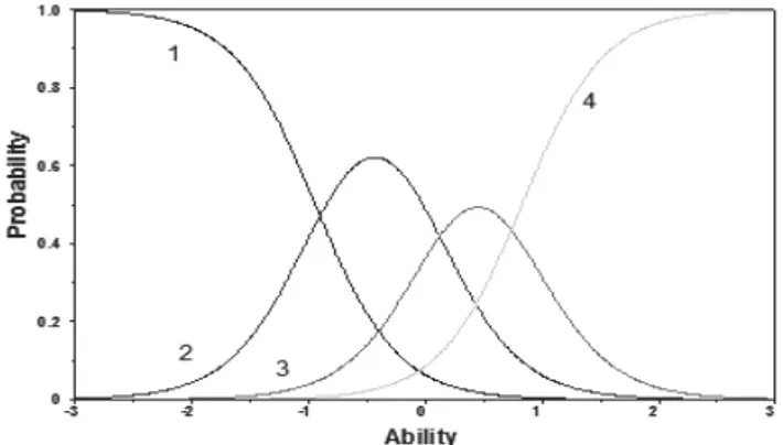
completely solve the items. This feature may cause difficulty in the estimation of abilities for very clever students. Furthermore, some parameters have large stan-dard errors, i.e. the parameters are not well estimated. This may happen with low selection frequency of the categories and when the items are not strongly related to the latent trait. In the difficulty range Contents and Simple application are at the bottom while Complex application turns out to be the most difficult argument. The slope parameters reflect the strength of the relation between the item and the la-tent ability: in this sense, positive and high α ’s are preferred. In the analysis, low values are observed for items 2, 3, 7 referring to the arguments Contents and Simple application while the highest values are noticed for items 5, 6 corresponding to Complex application. Therefore, the latter argument reflects an higher capability of differentiating among students respect to the other items. Items 5 and 6 concern the choice, calculation and comparison of variability measures. As an example, the category response curves for item 5 are shown in figure 1.
Figure 1 – Category response curves for item 5, 1st test.
Each curve expresses the probability of selecting the single response alternative as a function of ability. The responses are graded from 1 to 4, where 4 denotes the highest level in the item solving. As we can easily notice, the curve associated with alternative 4 has a monotonic increasing trend meaning that the probability of selecting the option increases as ability increases. On the contrary, the alterna-tive 1 has a monotonic decreasing trend, meaning that the probability of com-pletely failing the item approaches zero as ability increases. The intermediate re-sponse alternatives 2 and 3 have a non-monotonic trend, increasing for low and intermediate ability levels and decreasing on the rest of the domain. In fact, as ability increases, students are more likely to partially solve the item instead of fail-ing it. On the contrary, very capable students are more likely to perfectly solve the item instead of partially solving it.
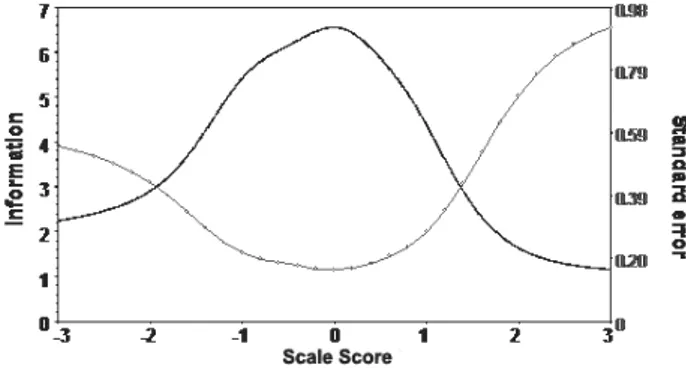
The item information should be considered to assess the informative and dis-crimination power of each single item. Figure 2 shows the information for the entire set of items, i.e. the test information curve (solid line), together with the correspondent measurement error curve (circle line).
The curves are rather symmetric on the ability range and the test is more in-formative and more precise for central scores. Furthermore, the precision of measurement especially decreases for high ability levels, accordingly to the results obtained for the threshold estimates. The single information curves are not re-ported but the highest contribution is given by items 5 and 6 (Complex application).
Figure 2 – Item Information and measurement error curve (1st examination).
Goodness of fit can be simply addressed by comparing the observed propor-tion of responses in each category and the model predicted values for all the items, as shown in table 2.
TABLE 2
Observed and expected response frequencies according to the GRM, 1st test
Item Cat. 1 Cat. 2 Cat. 3 Cat. 4
Obs. 0.0103 0.1795 0.8103 - 1 Exp. 0.0103 0.1793 0.8104 - Obs. 0.0667 0.0615 0.2205 0.6513 2 Exp. 0.0670 0.0621 0.2216 0.6493 Obs. 0.0103 0.0667 0.0513 0.8718 3 Exp. 0.0105 0.0684 0.0515 0.8696 Obs. 0.0923 0.2718 0.1231 0.5128 4 Exp. 0.0916 0.2681 0.1246 0.5157 Obs. 0.2103 0.3128 0.2359 0.2410 5 Exp. 0.2109 0.3142 0.2349 0.2400 Obs. 0.4000 0.1744 0.4256 - 6 Exp. 0.4062 0.1743 0.4195 - Obs. 0.0872 0.1231 0.0718 0.7179 7 Exp. 0.0883 0.1270 0.0726 0.7120 Obs. 0.3077 0.0923 0.6000 - 8 Exp. 0.3123 0.0928 0.5950 -
The small differences between the observed and the expected values seem to in-dicate a good fit of the model to data. A discussion about different methods of assessing goodness of fit in case of ordinal data can be found in Cagnone and Mignani (2004).
From table 2, the relative frequencies associated to each category of response can be observed to understand the response behaviour of students. All the items, except item 5, present the highest frequency in correspondence to the maximum
score (equal to 3 or 4). Both for item 5 and 6 the response frequencies are spread over the different categories, respect to the other items. This reflects the informa-tive power of the Complex application items and also highlights their complexity to be solved.
Analogous data analysis has been implemented for the remaining two tests. The second examination consists of 8 items, where items 1, 2, 6 have 3 response categories. A sample of 159 students has been analyzed. Table 3 shows the item parameter estimates for the GRM.
TABLE 3
Item parameter estimates for the 2ndtest (standard errors in brackets)
Item Argument α βi1 βi2 βi3 1 Contents 0.72 (0.50) -5.82 (3.51) -4.05 (2.45) - 2 Contents 0.79 (0.26) -2.56 (0.81) -0.95 (0.38) - 3 Simple application 1.22 (0.34) -2.03 (0.47) -1.46 (0.36) -1.10 (0.28) 4 Simple application 1.06 (0.32) -2.42 (0.62) -1.78 (0.45) -1.10 (0.31) 5 Complex application 1.42 (0.37) -2.52 (0.57) -2.19 (0.48) -1.33 (0.29) 6 Complex application 1.06 (0.30) -1.57 (0.41) -0.93 (0.29) - 7 Simple application 2.00 (0.38) -1.17 (0.20) -0.82 (0.15) -0.42 (0.13) 8 Interpretation 1.89 (0.33) -1.67 (0.27) -0.75 (0.15) 0.01 (0.14)
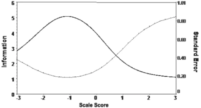
Again, Complex application items are associated with higher threshold parameters respect to the other items, reflecting the high ability needed to completely solve the problems. Items 7 and 8 regard probability. Low slope parameters are ob-served for Contents items while the highest values are noticed for items 5, 7, 8 cor-responding to Complex application. The results are coherent with the conclusions inferred from the first test. Figure 3 shows the test information and the meas-urement error curves.
Figure 3 – Item Information and measurement error curve (2nd examination).
The curve reflects the more informative capability for low ability levels. Most contribution is given by items 5, 7, 8.
Small differences between observed and expected frequencies, given in table 4, show a good fit of the GRM.
TABLE 4
Observed and expected response frequencies according to the GRM, 2ndtest
Item Cat. 1 Cat. 2 Cat. 3 Cat. 4
Obs. 0.0189 0.0440 0.9371 1 Exp. 0.0191 0.0443 0.9367 Obs. 0.1384 0.2013 0.6604 2 Exp. 0.1389 0.2015 0.6596 Obs. 0.1195 0.0755 0.0629 0.7421 3 Exp. 0.1210 0.0760 0.0623 0.7407 Obs. 0.1006 0.0692 0.1069 0.7233 4 Exp. 0.1031 0.0693 0.1056 0.7220 Obs. 0.0566 0.0252 0.1132 0.8050 5 Exp. 0.0579 0.0262 0.1130 0.8030 Obs. 0.2013 0.1069 0.6918 6 Exp. 0.2025 0.1067 0.6908 Obs. 0.1887 0.0818 0.1069 0.6226 7 Exp. 0.1884 0.0795 0.1073 0.6248 Obs. 0.1069 0.1761 0.2201 0.4969 8 Exp. 0.1107 0.1778 0.2152 0.4964
The observed proportions reveal that all arguments present the highest frequency associated with the last category.
Finally, the third test is considered. In this case, only the third item is scored through 3 response categories instead of 4. The test has been submitted to 145 students. The sample size is decreasing in the three tests, because most students who failed in the previous test decided to skip the following examination.
The item parameter estimates according to the GRM are shown in table 5. TABLE 5
Item parameter estimates for the 3rdtest (standard errors in brackets)
Item Argument α βi1 βi2 βi3 1 Contents 0.59 (0.47) -8.23 (6.55) -5.35 (3.77) -0.99 (0.76) 2 Contents 0.73 (0.38) -6.69 (4.07) -4.41 (2.24) -1.45 (0.72) 3 Simple application 0.62 (0.59) -5.88 (4.16) -3.45 (2.48) - 4 Simple application 1.39 (0.35) -3.03 (0.71) -1.59 (0.37) -0.35 (0.19) 5 Complex application 1.72 (0.36) -2.40 (0.52) -1.42 (0.28) -0.36 (0.16) 6 Complex application 3.72 (0.99) -1.53 (0.25) -1.17 (0.16) -0.84 (0.11) 7 Simple application 5.49 (1.19) -1.31 (0.18) -0.94 (0.12) -0.70 (0.08) 8 Interpretation 6.26 (1.19) -0.95 (0.11) -0.51 (0.07) -0.02 (0.07)
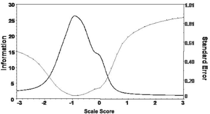
In this test, 5 items out of 8 are classified as Complex application. Nevertheless, we have found out that the first two items behave differently respect to the other items in the same argument. In particular, they present a low slope parameter and extreme low thresholds for the lower categories, even if the β parameter associ-ated with the last step is quite high. The topic of these items is probability: clearly, students found out the computational problem easier respect to the statistical in-ference problems associated with the remaining items of the same argument. Ex-tremely high slope parameters are noticed for items 6, 7, 8. The test information curve is shown in figure 4, together with the measurement error curve.
Figure 4 – Item Information and measurement error curve (3rd examination).
Again, the information curve is shifted on the left side of the ability range: the measurement is more precise for low-intermediate ability levels. Items 6, 7, 8 give the most contribution to the test information.
Goodness of fit is assessed through the comparison between observed and ex-pected frequencies given in table 6.
TABLE 6
Observed and expected response frequencies according to the GRM, 3rdtest
Item Cat. 1 Cat. 2 Cat. 3 Cat. 4
Obs. 0.0069 0.0345 0.3103 0.6483 1 Exp. 0.0089 0.0377 0.3200 0.6334 Obs. 0.0069 0.0345 0.2207 0.7379 2 Exp. 0.0095 0.0379 0.2303 0.7222 Obs. 0.0276 0.0828 0.8897 3 Exp. 0.0303 0.0888 0.8809 Obs. 0.0276 0.1034 0.2414 0.6276 4 Exp. 0.0330 0.1260 0.2516 0.5894 Obs. 0.0345 0.0897 0.2414 0.6345 5 Exp. 0.0486 0.1102 0.2398 0.6015 Obs. 0.0552 0.0414 0.0690 0.8345 6 Exp. 0.0845 0.0618 0.0773 0.7764 Obs. 0.0690 0.0552 0.0621 0.8138 7 Exp. 0.1065 0.0801 0.0655 0.7478 Obs. 0.1241 0.1241 0.2069 0.5448 8 Exp. 0.1825 0.1280 0.1797 0.5097
The differences are small and the GRM seems to recover the data well. All ar-guments present the highest frequency associated with the last category.
Finally, the student abilities in the three tests are taken into account. The evaluation of student performance has been largerly considered, see for example Cagnone et al. (2004), and Mignani et al. (2005). A rigorous comparison of the student performance in the tests would have been possible with longitudinal data, pre-calibrated items or test equating. In the first case, the same items should have been submitted to students at different time points. In the second case, the item properties should have been stably estimated in advance respect to a common la-tent ability. In the last case, the three tests should have contained some common
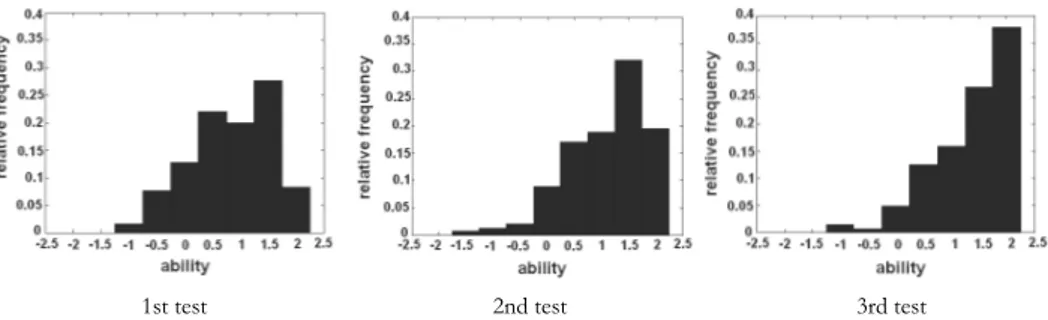
items as anchor terms. Test equating procedures in the IRT framework are de-scribed in Hambleton and Swaminathan, 1985. In the present work, the data are analyzed ex post and only a rough comparison of the three tests is possible. The Maximum A Posteriori (MAP) scores have been computed for the three samples of students. The ability distribution is presented for the three test in figure 5. The histograms suggest for all the tests that higher frequencies are present for high ability levels respect to low ones. In particular, the distribution is noticed to shift to the right from the first to the last test. Rigorous data collection and analyses are certainly needed to better investigate the growth of student learning during the course time.
1st test 2nd test 3rd test
Figure 5 – Histogram of estimated abilities in the three tests.
5. CONCLUSIONS
In this work, the GRM has been successfully applied to data coming from three tests submitted to students about basic Statistics. The model allowed a deep analysis of the item properties, showing the discrimination capability of the single items and arguments. In particular, Complex application has been highlighted as the most informative argument, able to catch the individual differences. The relative difficulties of the single steps within the items have been evaluated, showing meaningful differences in the arguments. Finally, improvement in the student performance has been noticed, with reference to the histograms of estimated abilities. Changes in the teaching process have been introduced during the course, increasing the complex application exercises. This may explain the students’ pro-gress, together with the self-selection through the three tests.
ACKNOWLEDGEMENTS
The authors would like to thank Prof. Stefania Mignani for her useful remarks and suggestions.
Dipartimento di Scienze Statistiche “P. Fortunati” MARIAGIULIAMATTEUCCI
REFERENCES
F.B. BAKER(1992), Item response theory parameter estimation techniques, Marcel Dekker, New York.
D. BARTHOLOMEW, M. KNOTT(1999),Latent variable models and factor analysis,Arnold Publishers, London.
S. CAGNONE, S. MIGNANI, R. RICCI, G. CASADEI, S. RICUCCI(2004),Computer-automated testing: an evaluation of undergraduate student performance, “Proceedings of Technology Enhanced Learning”,Kluwer Academic Publishers.
S. CAGNONE, R. RICCI(2005),Student ability assessment based on two IRT models,“Metodolŏski zvezki”, 2, pp. 209-218.
S.E. EMBRETSON, S.P. REISE(2000),Item response theory for psychologists,Lawrence Erlbaum Asso-ciates, Mahwah-New Jersey.
I. GAL, G.B. GARFILED(1997),The assessment challenge in the statistical education,IOS Pres, Am-sterdam.
R.K. HAMBLETON, H. SWAMINATHAN(1985), Item response theory,Kluwer–Nijhoff Publishing, Boston.
K. JÖRESKOG, I. MOUSTAKI(2001), Factor analysis of ordinal variables: a comparison of three ap-proaches,“Multivariate Behavioral Research”,36,pp. 347-387.
F.M. LORD, M.R. NOVICK(1968),Statistical theories of mental test scores, Addison-Wesley, Reading,
MA.
G.N. MASTERS(1982),A Rasch model for partial credit scoring,“Psychometrika”,47,pp. 149-174. S. MIGNANI, S. CAGNONE(2004),A comparison among different solutions for assessing the goodness of fit
of a generalized linear latent variable model for ordinal data,“Statistica Applicata”,16,pp. 1-19. S. MIGNANI, S. CAGNONE, G. CASADEI, A. CARBONARO(2005),An item response theory model for stu-dent ability evaluation using computer-automated test results.In Vichi, Monari, Mignani, Mon-tanari (Eds.): New developments in classification, data analysis, and knowledge organisation, Springer-Verlag, Berlin-Heidelberg, pp. 325-332.
I. MOUSTAKI(2000),A latent variable model for ordinal variables, “Applied Psychological
Meas-urement”,24,pp. 211-223.
F. SAMEJIMA(1969),Estimation of ability using a response pattern of graded scores,“Psychometrika Monograph”,17.
D. THISSEN(2003),Multilog 7.0. Multiple, categorical item analysis and test scoring using item response theory,Scientific Software International, Lincolnwood, IL.
W.J. VAN DER LINDEN, R.K. HAMBLETON(1997),Handbook of modern item response theory, Springer-Verlag, New York.
RIASSUNTO
Una proposta di stima dell’abilità dello studente attravero il Graded Response Model
Negli ultimi anni, la Facoltà di Scienze Politiche dell’Università di Bologna ha avviato, per alcuni corsi, un programma di riorganizzazione della didattica, introducendo più pro-ve intermedie di valutazione durante il processo di apprendimento. Valutare lo studente prima della prova finale ha il duplice scopo di misurare l’abilità raggiunta dallo studente e l’efficacia del processo di insegnamento in corso, al fine di poterlo riadattare simultanea-mente alle esigenze degli studenti. E’ in un tale sistema valutativo, comune ai paesi Anglo-sassoni, che l’Item Response Theory (IRT) esprime appieno le sue potenzialità. In questo lavoro, è stato considerato un modello di IRT per variabili politomiche ordinate al fine di
investigare le proprietà delle domande e di valutare il livello di rendimento dello studente. In particolare, viene applicato il Graded Response Model (GRM) nell’analisi di tre prove scritte intermedie del corso di Statistica di base. I risultati evidenziano la diversa composi-zione degli items e forniscono una descricomposi-zione immediata della distribucomposi-zione dell’abilità dello studente.
SUMMARY
Student assessment via graded response model
Recently, the Faculty of Political Science at the University of Bologna has started a program of didactics reorganization for several courses, introducing more than one evaluation test during the learning process. Student assessment before the final examina-tion has the double aim of measuring both the level of student’s ability and the effective-ness of the teaching process, in order to correct it real-time. In such an evaluation system, common to the Anglo-Saxon countries, Item Response Theory (IRT) expresses its effec-tiveness fully. In this paper, an IRT model for ordered polytomous variables is considered in order to investigate the item properties and to evaluate the student achievement. Par-ticularly, the Graded Response Model (GRM) is taken into account in the analysis of three different written tests of a basic Statistics course. The results highlight the different composition of the items and provide a simple description of the student ability distribu-tion.