Logic learning and optimized drawing: two hard combinatorial problems

(1)

Logic Learning and Optimized

Drawing: Two Hard Combinatorial

Problems

Tommaso Pastore

Dep. of Mathematics and Applications, "R. Caccioppoli"

University of Napoli, "Federico II"

Thesis submitted for the degree of

Doctor of Philosophy

Supervisor:

(2)

(3)

List of figures

1.1 Mindmap representing the structure of the thesis. . . 2

1.2 Circular representation of a graph [27]. . . 4

1.3 Strategic multistage scenario tree with tactical multiperiod graphs rooted with strategic nodes. . . 6

1.4 Optimal drawing for crossing minimization of a given graph. . . 7

1.5 Optimal drawing for crossing minimization of the incremented graph. . . . 8

2.1 A generic GRASP for a minimization problem. . . 16

2.2 Pseudo-code of the GRASP construction phase. . . 17

2.3 Empirical analysis of frequencies of the solutions. . . 19

2.4 Fitting data procedure. . . 19

2.5 Improve probability procedure. . . 20

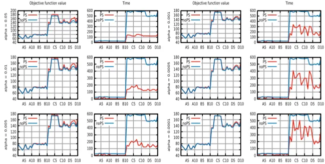
2.6 Experimental evaluation of the probabilistic stopping rule. In each boxplot, the boxes represent the first and the second quartile; solid line represent median while dotted vertical line is the full variation range. Plots vary for each threshold α. The dots connected by a line represent the mean values. 25 2.7 Comparison of objective function values and computation times obtained with and without probabilistic stopping rule for different threshold values. . 26

2.8 The phased local search procedure used in our GRASP. . . 28

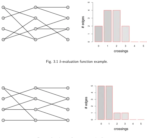
3.1 δ-evaluation function example. . . 38

3.2 δ-evaluation function example after swap. . . 38

3.3 Main Tabu algorithm. . . 39

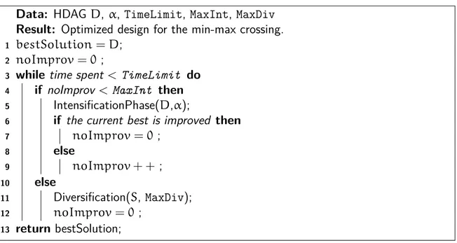
3.4 Pseudo-code of the Intensification Phase. . . 40

3.5 Pseudo-code of the Diversification Phase. . . 41

3.6 Comparison of δ and min-max objective functions. . . 47

3.7 Graphviz drawing of a simple hierarchical graph. . . 52

(6)

vi List of figures

3.9 Project management example. . . 54

3.10 Example optimized with a previous method. . . 55

3.11 Graph to illustrate the C2 method. . . 61

3.12 Initial partial solution. . . 61

3.13 Partial solution in an iteration of C2 construction phase. . . 62

3.14 Partial solution after an iteration of C2 construction phase. . . 62

3.15 Constructive phase C3 for the C-IGDP. . . 63

3.16 Swapping phase in local search for C-IGDP. . . 65

3.17 Initial solution. . . 66

3.18 Local search procedure. Left: Swap phase. Right: Insertion phase. . . 66

3.19 Example of the Path Relinking procedure. . . 67

3.20 Scatter Plot for two different instances. . . 73

3.21 Performance profile for three GRASP implementation and a TS. . . 74

3.22 GRASP3+PR Search Profile. . . 76

3.23 Search Profile. . . 77

3.24 Time to target plot. . . 82

3.25 Example optimized with new method. . . 82

4.1 Differences in the selection processes of the classic GRASP (a) and the BR-GRASP (b). . . 88

4.2 Flowchart of our SimGRASP algorithm. . . 89

4.3 Comparison of a MS simheuristic, SimGRASP with BR, and SimGRASP without BR. . . 92

4.4 Reoptimization problems hierarchy. . . 95

5.1 Representation of the stress constraints with asymmetrical traction (σ+) and compression (σ−) bounds. . . 105

5.2 General outline of the iterative topology optimization algorithm. . . 106

5.3 Representation of the case study considered in the experimental phase. . . 111

5.4 Representation of the load scheme considered in the experimental phase. . 111

5.5 Fixed load analysis: Class 20/25. . . 113

5.9 Proportional load analysis: Class 20/25. . . 117

(7)

List of figures vii

5.13 VMS comparison: case σ′ vms . . . 120 5.14 VMS comparison: case σ′′ vms . . . 120 5.15 VMS comparison: case σ′′′ vms . . . 120

(8)

(9)

List of tables

1.1 Hierarchical Graphs applications as listed in [119]. . . 5

2.1 Comparison between GRASP and other solvers. . . 23

2.2 Probabilistic stop on instances A, B, C and D. . . 24

2.3 Average of the solution values (avg-z) and execution time (avg-t) of the algorithms. The p subscript specifies when the implementation uses proposition 1. . . 29

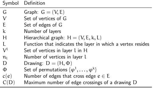
3.1 Symbols and Definitions. . . 34

3.2 Benchmark set. . . 43

3.3 Fine-Tune parameter α for the TS procedure. . . 45

3.4 Fine-Tune parameter tenure for the TS procedure. . . 45

3.5 TS fine-tune on 10 low density instances. . . 45

3.6 TS fine-tune on 16 high density instances. . . 46

3.7 Comparison of TS, MCE, and CPLEX on 49 instances (low density). . . 48

3.8 Comparison of MCE, SO, and TS on 60 instances (high density). . . 49

3.9 Summary of heuristics performance. . . 49

3.10 Analysis of both objective on 60 high-density instances. . . 51

3.11 Symbols and Definitions. . . 58

3.12 Fine-Tune parameter α for the constructive C1 procedure. . . 70

3.13 Fine-Tune parameter β for the constructive C4 procedure. . . 71

3.14 Performance comparison of the construction methods. . . 71

3.15 Comparison among different local search setups. . . 72

3.16 Performance comparison of GRASP variants and Tabu Search. . . 73

3.17 Comparison on entire benchmark set according to instance size . . . 78

3.18 Comparison on entire benchmark set according to K value . . . 79

3.19 Best values on very large instances, with K = 1. . . 80

3.20 Best values on very large instances, with K = 2. . . 80

(10)

x List of tables

4.1 Performance of BR-GRASP and SimGRASP for the VRP. . . 92

5.1 Material parameters considered in the fixed load experiment. . . 112

5.2 Solution properties obtained in the fixed load experiment. . . 112

5.3 Material parameters considered in the proportional load experiment. . . 114

5.4 Solution properties obtained in the proportional load experiment. . . 114

5.5 Solution properties obtained in the VMS comparison. . . 117

5.6 Comparison of solution properties obtained in the experiments with (w/) and without (w/o) displacement constraint. . . 119

(11)

Chapter 1 Introduction

Whether it be while surfing the Internet, registering financial transactions or processing medical records, we are constantly collecting new data. The process of information gathering, as acquisition of derived knowledge, substantially represents the basis of modern science and the foundation of the learning process itself. At the same time, the amount of data we

produce nowadays is unprecedented. According to a column featured on Forbes magazine1_,

there are 2.5 · 1018 bytes of data created each day, with the last two years alone that

generated the 90 percent of the data in the world. As a consequence of this, information extraction from large datasets or networks is a recurring operation in countless fields, establishing itself as a cornerstone process in an organic revolution that over the course of

time brought us from tally sticks2 _{to modern data centers.}

The purpose leading this thesis is to ideally follow the data flow along its journey, describing some hard combinatorial problems that arise from two key processes, one consecutive to the other: information extraction and representation. Moreover, having in mind the growing size of information networks, the approaches here considered will focus mainly on metaheuristic algorithms, to address the need for fast and effective optimization methods.

The core of this thesis is devoted to the study of Supervised Learning in Logic Domains and the Max Cut-Clique Problem, as examples of NP-hard data extraction processes, and two different Graph Drawing Problems. Moreover, stemming from these main topics, other additional themes will be addressed, namely two different approaches to handle Information Variability in Combinatorial Optimization Problems (COPs), and Topology Optimization

1_{Bernard Marr - “How Much Data Do We Create Every Day? The Mind-Blowing Stats Everyone Should}

Read”, Forbes Magazine - July 2018

2_{Grandell, Axel. "The reckoning board and tally stick." The Accounting Historians Journal 4.1 (1977):}

(12)

2 Introduction

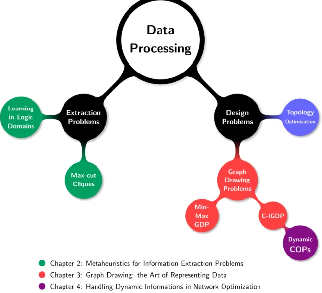
for the design of stress-constrained lightweight structures. The structure of the thesis and the interplays among its topics are depicted in Figure 1.1 and described in the following.

Data

Processing

Extraction Problems Learning in Logic Domains Max-cut Cliques Design Problems Graph Drawing Problems Min-Max GDP C-IGDP Dynamic COPs Topology Optimization

Chapter 2: Metaheuristics for Information Extraction Problems Chapter 3: Graph Drawing: the Art of Representing Data

Chapter 4: Handling Dynamic Informations in Network Optimization Chapter 5: Topology Optimization: a Hardly Constrained Design Problem

Fig. 1.1 Mindmap representing the structure of the thesis.

The first problem addressed in this thesis is logic supervised learning. In this scenario, studied in Chapter 2, we have a dataset of samples, each represented by a finite number of logic variables, and we show how a particular extension of the classic SAT problem –the Minimum Cost Satisfiability Problem (MinCost-SAT)– can be used to iteratively identify the different clauses of a compact formula in Disjunctive Normal Form (DNF), that possesses the desirable property of assuming the value True on one specific subset of the dataset and the value False on the rest.

(13)

3

The use of MinCost-SAT for learning propositional formulae from data is described in [48] and [151], and it proved to be very effective in several applications, particularly on those derived from biological and medical data analysis [10, 3, 155, 156, 154].

One of the main drawbacks of this approach lies in the difficulty of solving MinCost-SAT exactly or with an appropriate quality level. Such drawback is becoming more and more evident as, in the era of Big Data, the size of the datasets to analyze steadily increases. While the literature proposes both exact approaches ([63, 127], [151], and [153]) and heuristics ([138]), still the need for efficient MinCost-SAT solvers remains, and in particular for solvers that may take advantage of the specific structure of those MinCost-SAT representing supervised learning problems.

Chapter 2 will describe a GRASP-based metaheuristic algorithm designed to solve MinCost-SAT problems that arise in supervised learning. In doing so, we developed a new probabilistic stopping criterion that proves to be very effective in limiting the exploration of the solution space - whose explosion is a frequent problem in metaheuristic approaches. The method has been tested on several instances derived from artificial supervised problems in logic form, and successfully compared with four established solvers in the literature.

As a second example of information extraction problem, the second part of Chapter 2 studies the Max Cut-Clique Problem (MCCP). This problem is a variation of the classical Max Clique Problem with several applications in the area of market basket analysis. We formally describe the MCCP and detail the main characteristics of our hybrid heuristic solution strategy, presenting a comparison between our algorithm and the state-of-the-art.

Chapter 3 deals with data representation, introducing results obtained for two different Graph Drawing Problems (GDPs). Graph drawing is a well established area of computer science that consists in obtaining an automatic representation of a given graph, described in terms of its vertices and edges. In the scientific literature many aesthetic criteria have been proposed to identify the desirable properties that a good representation has to fulfill, with the most common being: edge crossings, graph area, edge length, edge bends, and symmetries. Their main objective is to achieve readable drawings in which it is easy to obtain or extract information. This goal is particularly critical in graphs with hundreds of vertices and edges, in which an improper layout could be extremely hard to analyze. The graph drawing area is very active, and an excellent resource on the topic is the book by Di Battista et al. [6], where many graph drawing models and related applications are introduced.

There are different drawing conventions to represent a graph. In some settings, the vertices of the graph are typically drawn in a circle, such as for example in genetic interaction networks. Figure 1.2 represents the two hundred and forty-five interactions found among 16

(14)

4 Introduction

Fig. 1.2 Circular representation of a graph [27].

micro-RNAs and 84 genes (see [27]). In other cases, the data has a clear sequential nature, like in workforce scheduling problems, where a set of tasks cannot be undertaken before the completion of some previous ones. Whenever the data is characterized by this kind of precedence relationships, the natural representation for the corresponding network is given by a hierarchical graph. Application fields which benefits from this graph layout can be found in Table 1.1. For example, in the field of operational inter-period material activities, a set of operational multi-period scenarios can be represented with a special graph rooted with replicas of the related strategic node, as it can be seen in Figure 1.3 (e.g see [47]).

The Hierarchical Directed Acyclic Graph (HDAG) representation is obtained by arranging the vertices on a series of equidistant vertical lines called layers in such a way that all edges point in the same direction. Note that working with hierarchies is not a limitation, since there exists a number of procedures to transform any directed acyclic graph (DAG) into a layered or hierarchical graph [5, 145].

The crossing minimization problem in hierarchical digraphs has received a lot of attention. Even the problem in bipartite graphs has been extensively studied for more than 40 years, beginning with the Relative Degree Algorithm introduced in Carpano [25]. Early heuristics were based on simple ordering rules, reflecting the goal of researchers and practitioners of

(15)

5

Context References Description

Workflow visualization [152] Representation of the work to be

exe-cuted by the project team.

Software engineering [29, 22] Representation of calling relationships

between subroutines in a computer pro-gram.

Database modeling [85] Definition of data connections and

sys-tem processing and storing diagrams.

Bioinformatics [98] Representations of proteins and other

structured molecules with multiple func-tional components.

Process modeling [81, 51] Analytical representation or illustration

of an organization’s business processes.

Network management [122, 92] Representation of the set of actions that

ensures that all network resources are put to productive use as best as possi-ble.

VLSI circuit design [13] Representation of the design of

inte-grated circuits (ICs) which are essential to the production of new semiconductor chips.

Decision diagrams [115, 116] Definition of logic synthesis and formal

verification of logic circuits.

Table 1.1 Hierarchical Graphs applications as listed in [119].

quickly obtaining solutions of reasonable quality. However, the field of optimization has recently evolved introducing complex methods, both in exact and heuristic domains. The crossing problem has benefited from these techniques, and advanced solution strategies have been proposed in the last 20 years to solve it. We refer the reader to Martí [113], Di Battista et al. [6], or Chimani et al. [30] to mention relatively recent developments.

In Chapter 3 we focus on two different variants of the crossing problem: (i) the min-max GDP [143], and (ii) the Constrained Incremental GDP.

The interest in the min-max GDP, originally called the bottleneck crossing minimization, arose in the context of VLSI circuits design in which it is more appropriate to minimize the maximum number of crossings over all edges (min-max) rather than the sum of the edge crossings over all the graph (min-sum). As stated in Bhatt and Leighton [13], an undesirable feature of VLSI layouts is the presence of a large number of wire crossings. More specifically, wires that are crossed by many others are susceptible to cross-talk, when all the crossing wires simultaneously carry the same signal, thus deteriorating the circuit

(16)

6 Introduction

Fig. 1.3 Strategic multistage scenario tree with tactical multiperiod graphs rooted with strategic nodes.

performance. On the other hand, if the number of wire crossings is small, the number of contact-cuts is also small, thus providing a better signal. Therefore, in order to attain a good performance over the network it is critical that no edge has a large number of crossings, more than the overall sum of crossings is small. Remarkably, the solution of the min-max problem is also useful in general graph drawing softwares, where zooming highlights a specific area of the graph where it is then desirable to have locally a low number of crossings.

On the other hand, the Constrained Incremental GDP (C-IGDP) is a variation of the classical min-sum GDP, that addresses the need of properly handling graph drawing in areas such as project management, production planning or CAD software, where changes

(17)

7

in project structure result in successive drawings of similar graphs. The so-called mental map of a drawing reflects the user’s ability to create a mental structure with the elements in the graph. When elements are added to or deleted from a graph, the user has to adjust their mental map to become familiar with the new graph. The dynamic graph drawing area is devoted to minimizing this effort. As described in [18], considering that a graph has been slightly modified, applying a graph drawing method from scratch would be inefficient and could provide a completely different drawing, thus resulting in a significant effort for the user to re-familiarize her/himself with the new map. Therefore, models to work with dynamic or incremental graphs have to be used in this context.

0 1 2 3 4 5 6 7 8 9 3 2 4 7 9 0 1 5 8 6 6 4 3 1 0 2 5 8 9 7 4 3 2 8 0 1 5 6 7 9 0 1 2 3 4 5 6 7 8 9

Fig. 1.4 Optimal drawing for crossing minimization of a given graph.

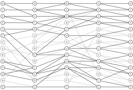
To illustrate the incremental problem, we consider the hierarchical drawing in Figure 1.4, which shows the optimal solution of the edge crossing minimization problem of a graph with 50 vertices and 5 layers. We increment this graph now by adding 20 vertices (4 in each layer), and their incident edges. Figure 1.5 shows the optimal solution of the edge crossing minimization problem of the new graph, where the new vertices and edges are represented with dotted lines.

Although the number of crossings in Figure 1.5 is minimum, 99, this new drawing was created from scratch, and it ignores the position of the vertices in the original drawing (the one in Figure 1.4). For example, vertex 6 in the first layer is in position 7 in Figure 1.4, but in position 10 in Figure 1.5. We can say that Figure 1.5 does not keep the mental map of the user familiarized with Figure 1.4. Therefore, in line with the dynamic drawing conventions [18], we propose reducing the number of crossings of the new graph while keeping the original vertices close to their positions in Figure 1.4.

Regarding hierarchical graphs, previous efforts only preserve the relative positions of the original vertices [106]. As will be shown, this can result in poor incremental drawings (i.e., the mental map of the drawing is not properly kept). The approach described in this thesis

(18)

8 Introduction 0 1 2 3 4 5 C A B 6 7 8 D 9 3 2 4 7 9 A C D 0 B 1 5 8 6 6 4 3 B 1 0 A 2 5 8 9 D C 7 4 3 2 8 A 0 B 1 C 5 6 D 7 9 0 1 2 3 4 A 5 B 6 C 7 8 D 9

Fig. 1.5 Optimal drawing for crossing minimization of the incremented graph.

considers a robust model with constraints on both the relative and the absolute position of the original vertices when minimizing the number of edge crossings in a sequence of drawings. In this way, we help the user to keep his or her mental map when working with a drawing where successive changes occur. In particular, our model restricts the relative position of the original vertices with respect to their position in the initial drawing (as in [106]), and also restricts their absolute position within a short distance of their initial position (as in [6] in the context of orthogonal graphs).

As in the case of the C-IGDP, a challenge of growing consideration in the operations research community consists in the inclusion of information variability in classical Combina-torial Optimization Problems. Given the non-deterministic nature of real-world scenarios, properly addressing information variability (or stochasticity) is essential for embedding optimization techniques into each of the supply-chain systems that determine production, scheduling, distribution, location-allocation, etc. Chapter 4 studies two iconic problems in the landscape of Dynamic Network Optimization: the Vehicle Routing Problem with stochastic demands, and the Reoptimization of Shortest Paths; presenting a simheuristic approach for the former, and surveying the research efforts made in the latter.

The vast majority of combinatorial problems are computationally intractable by nature, and the Vehicle Routing Problem (VRP) is no exception. For a summary of the existing approaches to solving the classical VRP, we refer the reader to three excellent resources on the topic: [149], [95], and [75]. Due to the complexity of the VRP, the typical solution techniques for large-scale instances mainly belong to the class of heuristic and metaheuristic algorithms. In our approach we embrace the Simheuristic paradigm, in which heuristic

(19)

9

algorithms are hybridized with a multi-stage Monte Carlo simulation to properly evaluate solution quality. More specifically, we couple a GRASP with biased randomization (BR-GRASP) with stochastic simulation in order to obtain reliable and competitive routing plans when considering customers with stochastic demands.

On the other hand, the Shortest Path Problem (SPP) established itself as one of the most representative and widespread polynomially solvable problems of operations research. Reoptimizing shortest paths on dynamic graphs consists in the solution of a sequence of shortest path problems, where each problem differs only slightly from the previous one. Each problem could be simply solved from scratch, independently from the previous one, by using either a label-correcting or a label-setting shortest path algorithm. Nevertheless, ad-hoc algorithms can efficiently use information gathered in previous computations and speed up the solution process.

If in Chapter 3 we address the problem of designing an optimized representation for information networks, Chapter 5 presents a solution for a different kind of design problem: the shaping of lightweight stress-constrained structures by means of Topology Optimization. Topology optimization is the most broad form of structural optimization. In general terms it aims at determining efficient material layouts within a given design space, starting from very few prescribed specifications such as load case and boundary conditions [134].

The development of additive manufacturing (AM) and 3D printing technologies makes possible to produce extremely complex structures which until recently, using traditional production methods, would have been impossible to accomplish or would require unreliable efforts and unacceptable costs. Component design by means of topology optimization from the earliest stages of their conceptual development could lead to major breakthroughs, maximizing the potential of 3D printing.

More specifically, in Chapter 5 we consider the topology optimization of Reinforced Concrete (RC) elements. In this scope, the primary goal for designers is to obtain the lightest structure while having a straight control on the stress levels. It is possible to notice how most of the optimization methods are limited to compliance minimization problems. This problem is considered classical in the optimization community and simpler to be solved if compared to the stress constrained one. Stress problems, indeed, bear more challenging difficulties, such as high non-linearity [124, 97]. On the other hand, even if some studies tackle the stress problem, in most of those cases the stress constraints there defined are based on the classical Von Mises stress, which is more appropriate to describe isotropic materials, such as steel, or other grouping strategies. See for example [43, 125, 144].

Chapter 5 provides a formal description of the structural optimization problem of interest, with particular emphasis on the form used in the imposition of the stress constraints, and

(20)

10 Introduction

presents an iterative heuristic algorithm with its solutions for a wide range of load cases and material properties.

(21)

Chapter 2 Metaheuristics for Information

Extraction Problems

Right after being collected and appropriately stored, a data stream is ready to start its journey and be processed, to extract its most relevant informations and recurring patterns. The focus of the present Chapter consists in the study of the contributions that operations research –and more specifically metaheuristic techniques– can bring in the solutions of two widely different mining problems. The problems of interest are respectively concerned with the extraction of boolean formulae in supervised learning, and the study of special cliques in graphs of large size.

2.1 From Logic Learning to Minimum Cost

Satisfiability

The goal of logic supervised learning consists in inductively determining separations among sets of data, starting from a set of labeled training observations. The approach adopted in this thesis, as described in [48] and applied in [49], reduces the learning problem to a sequence of satifiability instances.

The logic data, or the observations to be used in the in the inductive learning process, are defined as vectors r ∈ {−1, 0, 1}n, and called records. In contrast with classical Boolean

vectors, the components rican not only indicate the presence (ri = 1) or absence (ri = −1)

of a certain feature i, but additionally include the possibility of an absence of informations (ri = 0).

For each of such records, we define index sets r+, r−, and r0, containing the indices

(22)

12 Metaheuristics for Information Extraction Problems

r comes a logic outcome, either True or False, to represent the presence or absence of a

given property in the observation. We collect the records r for which the property is absent in a set A, and those for which it is present in a set B.

The aim in this supervised learning scenario is to extract a Boolean formula from the observation records, that completely separates the set of positive examples B from the set

A. This separation process takes places by means of a set of vectors, called “separating set”.

To properly define the concept of separation, we introduce the property of being nested.

Let f be a {−1, 0, 1}n _{vector, then f is said to be nested in a {−1, 0, 1}}n _{vector g, if}

and only if for any fi equal to 1 or −1, the corresponding entry of g , gi, is such that

gi = fi. Conversely, f is not nested in g if and only if there is a fi = 1 in f, such that

gi = −fi or gi = 0.

On the base of the nested relation we are able to define separation.

Let A and B be sets of records of the same size n. A record s separates b ∈ B from A if and only if

S1. s is not nested in a, ∀a ∈ A; S2. s is nested in b.

Then, a set of records S separates the whole set B from A if, for each record s ∈ S, s

is not nested in any a ∈ A, and for each b ∈ B it exists a sb ∈ Ssuch that sb separates

b from A. As proven in [48], the existence of such a separating set S of B from A is

guaranteed if and only if no record b ∈ B is nested in any record a ∈ A.

The use of satisfiability models for learning propositional formulae gathered several successes, as reported in [10, 3, 155, 156, 154]. In the following we describe how to obtain a specific variation of the classical SAT, the Minimum Cost Satisfiability Problem (MinCostSAT), to model supervised learning in Logic Fields.

Let A and B be non-empty sets of {−1, 0, 1}n records. The core idea of this approach

is to iteratively find logic records s to separate a growing portion B∗ _{⊆ B}_{from A, until a}

separating set S is obtained.

To write a proper satisfiability model we introduce for each i = 1, . . . , n two Boolean

variables, pi and qi. These variables are tightly connected with the component of the

separating vector s to be found, in the sense that

si = 1, if pi = True∧ qi = False;

si = −1, if pi = False∧ qi = True;

si = 0 if pi = qi = False.

(23)

2.1 From Logic Learning to Minimum Cost

Satisfiability 13

The case pi = qi = Truehas not a clear interpretation, so it is ruled out enforcing

¬pi∨ ¬qi, ∀i = 1, . . . , n. (2.2)

Since s is a separating vector, it has to fulfill conditions S1 and S2. In the following we take into account those two separately, and obtain two different set of constraints to be included in our SAT model.

Condition S1 requires that s is not nested in any a ∈ A. This means that exists at least an index i such that one of the three following conditions happens:

• ai = 1and si = −1;

• ai = −1 and si = 1;

• ai = 0and si = 1∨ si = −1.

So, for this index i, in terms of pi and qi, using 2.1 and 2.2 we obtain

ai = 1⇒ qi

ai = −1⇒ pi

ai = 0⇒ qi∨ pi.

(2.3) Since these three conditions have to hold for each a ∈ A and at least an index i, they can be collected in the following disjunctions:

  _ i∈a+_∪a0 qi  ∨   _ i∈a−_∪a0 pi  , ∀a ∈ A (2.4)

that completely enclose condition S1. On the other hand, to take into account condition S2, we have that if s separates a record b ∈ B, s has to be nested in b. Following a similar approach to the one presented for condition S1, we have

bi = 1⇒ ¬qi

bi = −1⇒ ¬pi

bi = 0⇒ ¬pi∨ ¬qi

(2.5) At the same time, in our pursuit for a separating record s, there is no guarantee that a single record is able to separate all the elements of B from A. For this reason, it is not possible to include, for each b ∈ B, (2.5) as constraint in a satisfiability model. As

(24)

whether s must separate b from A. More specifically, db = Truemeans that s needs not

to separate b from A, while db = False requires that separation. Using variable db in

(2.5), we get to the new following form

¬qi∨ db, ∀i ∈ b+∪ b0

¬pi∨ db, ∀i ∈ b−∪ b0.

(2.6) As mentioned earlier, the idea behind this approach is to decompose the problem of finding a separating set into a sequence of subproblems, each of which determines a vector

s that separates a nonempty subset of B from A. This idea can be translated in an

optimization problem if at each step we try to maximize the number of elements of B

separated from A. Rendering this insight in terms of variables db, we want a separating

record s, i.e. a vector that satisfies (2.4) and (2.6), and that does so with the minimal

number of db variables with a True value.

For each b ∈ B, we define a cost function cb(db) that is equal to 1 if db is True, and

0 otherwise. Using the costs cb and in light of constraints (2.4) and (2.6), we obtain the

following Satisfiability Problem:

z =minX b∈B cb(db) subject to: _ i∈a+_∪a0 qi∨ _ i∈a−_∪a0 pi ∀a ∈ A ¬qi∨ db, ∀i ∈ b+∪ b0 ¬pi∨ db, ∀i ∈ b−∪ b0. (2.7)

Problems of this family are called Minimum Cost Satisfiability Problems. In their most general form they can be stated as follows.

Given a set of n Boolean variables X = {x1, . . . , xn}, a non-negative cost function

c : X 7→ R+ _{such that c(x}

i) = ci ≥ 0, i = 1, . . . , n, and a Boolean formula φ(X)

expressed in CNF, the MinCostSAT problem consists in finding a truth assignment for the variables in X such that the total cost is minimized while φ(X) is satisfied. Accordingly, the mathematical formulation of the problem is:

(25)

2.2 A GRASP for MinCostSAT 15 (MinCostSAT) z = min n X i=1 cixi subject to: φ(X) = 1, xi ∈{0, 1}, ∀i = 1, . . . , n.

It is easy to see that a general SAT problem can be reduced to a MinCostSAT problem

whose costs ci are all equal to 0. Furthermore, the decision version of the MinCostSAT

problem is NP-complete [63]. While the Boolean satisfiability problem is an evergreen in the landscape of scientific literature, MinCostSAT has received less attention.

2.2 A GRASP for MinCostSAT

GRASP is a well established iterative multistart metaheuristic method for difficult combina-torial optimization problems [50]. The reader can refer to [57, 58] for a study of a generic GRASP metaheuristic framework and its applications.

Such method is characterized by the repeated execution of two main phases: a construc-tion and a local search phase. The construcconstruc-tion phase iteratively adds one component at a time to the current solution under construction. At each iteration, an element is randomly selected from a restricted candidate list (RCL), composed by the best candidates, according to some greedy function that measures the myopic benefit of selecting each element.

Once a complete solution is obtained, the local search procedure attempts to improve it by producing a locally optimal solution with respect to some suitably defined neighborhood structure. Construction and local search phases are repeatedly applied. The best locally optimal solution found is returned as final result. Figure 2.1 depicts the pseudo-code of a generic GRASP for a minimization problem.

In order to allow a better and easier implementation of our GRASP, we treat the MinCost-SAT as particular covering problem with incompatibility constraints. Indeed, we consider each literal (x, ¬x) as a separate element, and a clause of the CNF is covered if at least one literal in the clause is contained in the solution. The algorithm tries to add literals to the solution in order to cover all the clauses and, once the literal x is added to the solution, then the literal ¬x cannot be inserted (and vice versa). Therefore, if the literal x is in solution, the variable x is assigned to true and all clauses covered by x are satisfied. Similarly, if the literal ¬x is in solution, the variable x is assigned to false, and clauses containing ¬x are satisfied.

(26)

1 Algorithm GRASP(β)

2 x∗ ← Nil ;

3 z(x∗)← +∞ ;

4 while a stopping criterion is not satisfied do

5 Build a greedy randomized solution x ;

6 x ← LocalSearch(x) ;

7 if z(x) < z(x∗) then

8 x∗ ← x ;

9 z(x∗)← z(x) ;

10 return x∗

Fig. 2.1 A generic GRASP for a minimization problem.

The construction phase adds a literal at a time, until all clauses are covered or no more literals can be assigned. At each iteration of the construction, if a clause can be covered only by a single literal x – due to the choices made in previous iterations – then x is selected to cover the clause. Otherwise, if there are not clauses covered by only a single literal, the addition of literals to the solution takes place according to a penalty function, penalty(·), which greedily sorts all the candidates literals, as described below.

Let cr(x) be the number of clauses yet to be covered that contain x. We then compute:

penalty(x) = c(x) + cr(¬x)

cr(x) . (2.8)

This penalty function evaluates both the benefits and disadvantages that can result from the choice of a literal rather than another. The benefits are proportional to the number of uncovered clauses that the chosen literal could cover, while the disadvantages are related to both the cost of the literal and the number of uncovered clauses that could be covered by ¬x. The smaller the penalty function penalty(x), the more favorable is the literal x. According to the GRASP scheme, the selection of the literal to add is not purely greedy, but a Restricted Candidate List (RCL) is created with the most promising elements, and an element is randomly selected among them. Concerning the tuning of the parameter β, whose task is to adjust the greediness of the construction phase, we performed an extensive analysis over a set of ten different random seeds. Such testing showed how a nearly totally greedy setup (β = 0.1) allowed the algorithm to attain better quality solutions in smallest running times.

Let |C| = m be the number of clauses. Since |X| = 2n, in the worst case scenario the loop while (Figure 2.2, line 3) in the construct-solution function pseudo-coded

(27)

2.2 A GRASP for MinCostSAT 17

1 Function construct-solution(C, X, β)

/* C is the set of uncovered clauses */

/* X is the set of candidate literals */

2 s ← ∅ ;

3 while C ̸= ∅ do

4 if c ∈ C can be covered only by x ∈ X then

5 s ← s ∪ {x}; 6 X← X \ {x, ¬x}; 7 C ← C \ {¯c | x ∈ ¯c}; 8 else 9 compute penalty(x) ∀ x ∈ X; 10 th← min

x∈X{penalty(x)} + β(maxx∈X{penalty(x)} − minx∈X{penalty(x)}) ;

11 RCL← { x ∈ X: penalty(x) ≤ th } ; 12 x^← rand(RCL) ; 13 s ← s ∪ {^x}; 14 X← X \ {^x, ¬^x}; 15 C ← C \ {¯c | ^x ∈ ¯c}; 16 return s

Fig. 2.2 Pseudo-code of the GRASP construction phase.

in Fig. 2.2 runs m times and in each run the most expensive operation consists in the construction of the RCL. Therefore, the total computational complexity is O(m · n).

In the local search phase, the algorithm uses a 1-exchange (flip) neighborhood function, where two solutions are neighbors if and only if they differ in at most one component. Therefore, if there exists a better solution ¯x that differs only for one literal from the current solution x, the current solution s is set to ¯s and the procedure restarts. If such a solution does not exists, the procedure ends and returns the current solution s. The local search procedure would also re-establish feasibility if the current solution is not covering all clauses of φ(X). During our experimentation we tested the one-flip local search using two different neighborhood exploration strategies: first improvement and best improvement. With the former strategy, the current solution is replaced by the first improving solution found in its neighborhood; such improving solution is then used as a starting point for the next local exploration. On the other hand, with the best improvement strategy, the current solution x is replaced with the solution ¯x ∈ N (x) corresponding to the greatest improvement in terms of objective function value; ¯x is then used as a starting point for the next local exploration. Our results showed how the first improvement strategy is slightly faster, as expected, while attaining solution of the same quality of those given by the best improvement strategy.

(28)

Based on this rationale, we selected first improvement as exploration strategy in our testing phase.

2.3 Bernoulli Take the Wheel! A probabilistic

Stop-ping Rule

Although being very fast and powerful, most metaheuristics present a shortcoming in the effectiveness of their stopping rule. Usually, the stopping criterion is based on a bound on the maximum number of iterations, a limit on total execution time, or a given maximum number of consecutive iterations without improvement. In this algorithm, we propose a probabilistic stopping criterion, inspired by [132].

The stopping criterion is composed of two phases, described in the next subsections. It can be sketched as follows. First, let X be a random variable representing the value of a solution obtained at the end of a generic GRASP iteration. In the first phase – the

fitting-data procedure – the probability distribution fX(·) of X is estimated, while

during the second phase – improve-probability procedure – the probability of obtaining an improvement of the current solution value is computed. Then, accordingly to a threshold, the algorithm either stops or continues its execution.

The first step to be performed in order to properly represent the random variable X with a theoretical distribution consists in an empirical observation of the algorithm. Examining the objective function values obtained at the end of each iteration, and counting up the respective frequencies, it is possible to select a promising parametric family of distributions. Afterwards, by means of a Maximum Likelihood Estimation (MLE), see for example [137], a choice is made regarding the parameters characterizing the best fitting distribution of the chosen family.

In order to carry on the empirical analysis of the objective function value obtained in a generic iteration of GRASP, which will result in a first guess concerning the parametric family of distributions, we represent the data obtained in the following way.

Let I be a fixed instance and F the set of solutions obtained by the algorithm up to the current iteration, and let Z be the multiset of the objective function values associated to F. Since we are dealing with a minimization problem, it is harder to find good quality solutions, whose cost is small in term of objective function, rather than expensive ones. This means that during the analysis of the values in Z we expect to find an higher concentration of elements between the mean value µ and the max(Z). In order to represent the values in Z with a positive distribution function, that presents higher frequencies in a right neighborhood

(29)

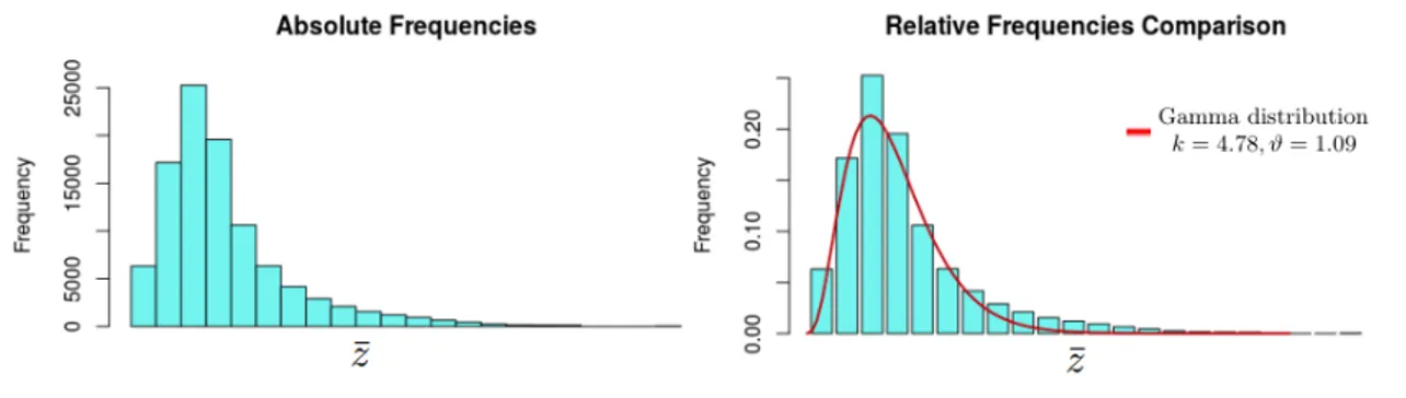
2.3 Bernoulli Take the Wheel! A probabilistic Stopping Rule 19

Fig. 2.3 Empirical analysis of frequencies of the solutions.

1 Function fitting-data( ¯Z)

/* ¯Z is the initial sample of the objective function values */

2 foreach z ∈ ¯Z do

3 z =max( ¯Z) − z;

4 {k, θ} ← MLE(Z, "gamma");

5 return {k, θ}

Fig. 2.4 Fitting data procedure.

of zero and a single tail which decays for growing values of the random variable, we perform a reflection on the data in Z by means of the following transformation:

¯z = max(Z) − z, ∀ z ∈ Z. (2.9)

The behavior of the distribution of ¯z in our instances has then a very recognizable behavior. A representative of such distribution is given in Figure 2.3 where the histogram of absolute and relative frequencies of ¯z are plotted. It is easy to observe how the gamma distribution family represents a reasonable educated guess for our random variable.

Once we have chosen the gamma distribution family, we estimate its parameters performing a MLE. In order to accomplish the estimation, we collect an initial sample of solution values and on-line execute a function, developed in R (whose pseudo-code is reported in Figure 2.4), which carries out the MLE and returns the characteristic shape and scale parameters, k and θ, which pinpoint the specific distribution of the gamma family that best suits the data.

The second phase of the probabilistic stop takes place once that the probability

(30)

1 Function improve-probability(k, θ, z∗)

/* z∗ is the value of the incumbent */

2 p← pgamma(z∗, shape = k, scale = θ);

3 return p

Fig. 2.5 Improve probability procedure.

Let ^z be the best solution value found so far. It is possible to compute an approximation of the probability of improving the incumbent solution by

p = 1 −

Zmax(Z)−^z 0

fX(t) dt. (2.10)

The result of the procedures fitting-data and improve-probability consists in an estimate of the probability of incurring in an improving solution in the next iterations. Such probability is compared with a user-defined threshold, α, and if p < α the algorithm stops. More specifically, in our implementation the stopping criterion works as follows:

a) let q be an user-defined positive integer, and let ¯Z be the sample of initial solution

values obtained by the GRASP in the first q iterations;

b) call the fitting-data procedure, whose input is ¯Z is called one-off to estimate

shape and scale parameters, k and θ, of the best fitting gamma distribution;

c) every time that an incumbent is improved, improve-probability procedure (pseudo-code in Figure 2.5) is performed and the probability p of further improvements is computed. If p is less than or equal to α the stopping criterion is satisfied. For the purpose of determining p, we have used the function pgamma of R package stats.

2.4 Computational Testing I

Our GRASP has been implemented in C++ and compiled with gcc5.4.0 with the flag

-std=c++14. All tests were run on a cluster of nodes, connected by 10 Gigabit Infiniband

technology, each of them with two processors Intel Xeon E5-4610v2@2.30GHz.

We performed two different kinds of experimental tests. In the first one, we compared the algorithm with different solvers proposed in literature, without use of probabilistic stop. In particular, we used: Z3 solver freely available from Microsoft Research [34], bsolo solver kindly provided by its authors [101], the MiniSat+ [46] available at web page http:

(31)

2.4 Computational Testing I 21

//minisat.se/, and PWBO available at web page http://sat.inesc-id.pt/pwbo/index.html. The aim of this first set of computational experiment is the evaluation of the quality of the solutions obtained by our algorithm within a certain time limit. More specifically, the stopping criterion for GRASP, bsolo, and PWBO is a time limit of 3 hours, for Z3 and

MiniSat+ is the reaching of an optimal solution.

Z3 is a satisfiability modulo theories (SMT) solver from Microsoft Research that

generalizes Boolean satisfiability by adding equality reasoning, arithmetic, fixed-size bit-vectors, arrays, quantifiers, and other useful first-order theories. Z3 integrates modern backtracking-based search algorithm for solving the CNF-SAT problem, namely DPLL-algorithm; in addition it provides a standard search pruning methods, such as two-watching literals, lemma learning using conflict clauses, phase caching for guiding case splits, and performs non-chronological backtracking.

bsolo [101, 102] is an algorithmic scheme resulting from the integration of several

features from SAT-algorithms in a branch-and-bound procedure to solve the binate covering problem. It incorporates the most important characteristics of a branch-and-bound and SAT algorithm, bounding and reduction techniques for the former, and search pruning techniques for the latter. In particular, it incorporates the search pruning techniques of the Generic seaRch Algorithm-SAT proposed in [104].

MiniSat+[46, 142] is a minimalistic implementation of a Chaff-like SAT solver based

on the two-literal watch scheme for fast Boolean constraint propagation [117], and conflict clauses driven learning [104]. In fact the MiniSat solver provides a mechanism which allows to minimize the clauses conflicts. PWBO [110, 112, 111] is a Parallel Weighted Boolean Optimization Solver. The algorithm uses two threads in order to simultaneously estimate a lower and an upper bound, by means of an unsatisfiability-based procedure and a linear search, respectively. Moreover, learned clauses are shared between threads during the search.

In our testing, we have initially considered the datasets used to test feature selection methods in [11], where an extensive description of the generation procedure can be found. Such testbed is composed of 4 types of problems (A,B,C,D), for each of which 10 random repetitions have been generated. Problems of type A and B are of moderate size (100 positive examples, 100 negative examples, 100 logic features), but differ in the form of the formula used to classify the samples into the positive and negative classes (the formula being more complex for B than for A). Problems of type C and D are much larger (200 positive examples, 200 negative examples, 2500 logic features), and D has a more complex generating logic formula than C.

(32)

Table 2.1 reports both the value of the solutions and the time needed to achieve them

(in the case of GRASP, it is average over ten runs).1 _{For problems of moderate size (A}

and B), the results show that GRASP finds an optimal solution whenever one of the exact solvers converges. Moreover, GRASP is very fast in finding the optimal solution, although here it runs the full allotted time before stopping the search. For larger instances (C and D), GRASP always provides a solution within the bounds, while two of the other tested solvers fail in doing so and the two that are successful (bsolo, PWBO) always obtain values of inferior quality.

The second set of experimental tests was performed with the purpose of evaluating the impact of the probabilistic stopping rule. In order to do so, we have chosen five different

values for threshold α, two distinct sizes for the set ¯Z of initial solution, and executed

GRASP using ten different random seeds imposing a maximum number of iterations as stopping criterion. This experimental setup yielded for each instance, and for each threshold value, 20 executions of the algorithm. About such runs, the data collected were: the number of executions in which the probabilistic stopping rule was verified (“stops”), the

mean value of the objective function of the best solution found (µz), and the average

computational time needed (µt). To carry out the evaluation of the stopping rule, we

executed the algorithm only using the maximum number of iterations as stopping criterion for each instance and for each random seed. About this second setup, the data collected

are, as for the first one, the objective function of the best solution found (µ^z) and the

average computational time needed (µ^t). For the sake of comparison, we considered the

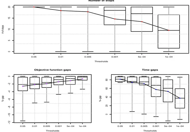
percentage gaps between the results collected with and without the probabilistic stopping rule. The second set of experimental tests is summarized in Table 2.2 and in Figure 2.7. For each pair of columns (3,4), (6,7), (9,10), (12, 13), the table reports the percentage of loss in terms of objective function value and the percentage of gain in terms of computation times using the probabilistic stopping criterion, respectively. The analysis of the gaps shows how the probabilistic stop yields little or no changes in the objective function value while bringing dramatic improvements in the total computational time.

The experimental evaluation of the probabilistic stop is summarized in the three distinct boxplots of Figure 2.6. Each boxplot reports a sensible information related to the impact of the probabilistic stop, namely: the number of times the probabilistic criterion has been satisfied, the gaps in the objective function values, and the gaps in the computation times obtained comparing the solutions obtained with and without the use of the probabilistic stopping rule. Such information are collected, for each instance, as averages of the data obtained over 20 trials in the experimental setup described above. The first boxplot depicts

(33)

2.4 Computational Testing I 23

Table 2.1 Comparison between GRASP and other solvers.

GRASP Z3 bsolo MiniSat+ pwbo-2T

Inst. Time Value Time Value Time Value Time Value Time Value

A1 6.56 78.0 10767.75 78.0 0.09 78.0 0.19 78.0 0.03 78.0 A2 1.71 71.0 611.29 71.0 109.59 71.0 75.46 71.0 121.58 71.0 A3 0.64 65.0 49.75 65.0 598.71 65.0 10.22 65.0 5.14 65.0 A4 0.18 58.0 4.00 58.0 205.77 58.0 137.82 58.0 56.64 58.0 A5 0.29 66.0 69.31 66.0 331.51 66.0 9.03 66.0 30.64 66.0 A6 21.97 77.0 5500.17 77.0 328.93 77.0 32.82 77.0 359.97 77.0 A7 0.21 63.0 30.57 63.0 134.20 63.0 19.34 63.0 24.12 63.0 A8 0.25 62.0 6.57 62.0 307.69 62.0 16.84 62.0 11.81 62.0 A9 12.79 72.0 1088.83 72.0 3118.32 72.0 288.76 72.0 208.63 72.0 A10 0.33 66.0 42.23 66.0 62.03 66.0 37.75 66.0 1.81 66.0 B1 6.17 78.0 8600.60 78.0 304.36 78.0 121.25 78.0 20.01 78.0 B2 493.56 80.0 18789.20 80.0 4107.41 80.0 48.21 80.0 823.66 80.0 B3 205.37 77.0 7037.00 77.0 515.25 77.0 132.74 77.0 1.69 77.0 B4 38.26 77.0 7762.03 77.0 376.00 77.0 119.49 77.0 1462.18 77.0 B5 19.89 79.0 15785.35 79.0 3025.26 79.0 214.52 79.0 45.05 79.0 B6 28.45 76.0 4087.14 76.0 394.45 76.0 162.31 76.0 83.72 76.0 B7 129.76 78.0 10114.84 78.0 490.30 78.0 266.25 78.0 455.92 81.0* B8 44.42 76.0 5186.45 76.0 5821.19 76.0 1319.21 76.0 259.07 76.0 B9 152.77 80.0 14802.00 80.0 5216.95 82.0 36.28 80.0 557.02 80.0 B10 7.55 73.0 1632.87 73.0 760.28 79.0 370.30 73.0 72.09 73.0 C1 366.24 132.0 86400 – 8616.25 178.0* 86400 – 343.38 178.0* C2 543.11 131.0 86400 – 323.90 150.0* 86400 – 1742.68 174.0* C3 5883.6 174.1 86400 – 6166.06 177.0* 86400 – 421.64 177.0* C4 4507.63 176.3 86400 – 6209.69 178.0* 86400 – 2443.20 177.0* C5 5707.51 171.2 86400 – 314.18 179.0* 86400 – 67.73 178.0* C6 6269.91 172.1 86400 – 1547.90 177.0* 86400 – 2188.82 177.0* C7 6193.15 165.9 86400 – 794.90 177.0* 86400 – 730.36 178.0* C8 596.58 137.0 86400 – 306.27 169.0* 86400 – 837.71 178.0* C9 466.3 136.0 86400 – 433.32 179.0* 86400 – 3455.92 178.0* C10 938.54 136.0 86400 – 3703.94 180.0* 86400 – 4617.24 179.0* D1 3801.61 145.3 86400 – 307.25 175.0* 86400 – 127.69 180.0* D2 2040.64 139.0 86400 – 7704.92 177.0* 86400 – 2327.23 177.0* D3 1742.78 143.0 86400 – 309.10 145.0* 86400 – 345.97 178.0* D4 1741.95 135.0 86400 – 6457.79 177.0* 86400 – 295.76 178.0* D5 1506.22 134.0 86400 – 6283.27 178.0* 86400 – 238.81 173.0* D6 1960.87 144.5 86400 – 309.11 173.0* 86400 – 2413.42 178.0* D7 1544.42 143.0 86400 – 4378.73 179.0* 86400 – 1250.07 178.0* D8 1756.15 144.0 86400 – 1214.97 179.0* 86400 – 248.85 179.0* D9 2779.38 137.0 86400 – 303.11 146.0* 86400 – 4.73 179.0* D10 5896.86 149.0 86400 – 319.45 170.0* 86400 – 1239.93 176.0* Y 16.05 0.0 0.73 0.0 9411.06 974* 1.96 0 0.23 0.0 *sub-optimal solution

– no optimal solution found in 24 hours

the number of total stops recorded for different values of threshold α. Larger values of

α, indeed, yield a less coercive stopping rule, thus recording an higher number of stops.

Anyhow, even for the smallest, most conservative α, the average number of stops recorded is close to 50% of the tests performed. In the second boxplot, the objective function gap is reported. Such gap quantifies the qualitative worsening in quality of the solutions obtained with the probabilistic stopping rule. The gaps yielded show how even with the highest α, the difference in solution quality is extremely small, with a single minimum of

(34)

Table 2.2 Probabilistic stop on instances A, B, C and D.

threshold α inst %-gap z %-gap t(s) inst %-gap z %-gap t(s) inst %-gap z %-gap t(s) inst %gap z %gap t(s)

5· 10−2 _A1 _-0.0 _83.1 _B1 _-2.1 _87.1 _C1 _-6.6 _76.0 _D1 _-5.0 _79.3 1· 10−2 _A1 _-0.0 _83.1 _B1 _-2.1 _87.1 _C1 _-6.6 _76.1 _D1 _-5.0 _79.3 5· 10−3 _A1 _-0.0 _83.0 _B1 _-2.1 _87.1 _C1 _-5.0 _74.8 _D1 _-4.9 _78.7 1· 10−3 _A1 _-0.0 _2.5 _B1 _-2.1 _87.1 _C1 _-3.8 _70.7 _D1 _-1.7 _58.9 5· 10−4 _A1 _-0.0 _-15.3 _B1 _-2.1 _87.2 _C1 _-2.6 _70.2 _D1 _-1.2 _49.0 1· 10−4 _A1 _-0.0 _-11.8 _B1 _-0.5 _86.1 _C1 _-1.3 _52.5 _D1 _-0.2 _31.6 5· 10−2 _A2 _-0.0 _84.0 _B2 _-0.7 _87.0 _C2 _-3.5 _76.0 _D2 _-0.1 _79.1 1· 10−2 _A2 _-0.0 _84.1 _B2 _-0.7 _87.0 _C2 _-3.5 _76.2 _D2 _-0.1 _79.1 5· 10−3 _A2 _-0.0 _83.6 _B2 _-0.7 _86.9 _C2 _-3.5 _76.7 _D2 _-0.1 _79.1 1· 10−3 _A2 _-0.0 _84.0 _B2 _-0.7 _87.0 _C2 _-1.9 _76.4 _D2 _-0.1 _79.1 5· 10−4 _A2 _-0.0 _84.9 _B2 _-0.7 _87.0 _C2 _-1.9 _76.1 _D2 _-0.1 _75.7 1· 10−4 _A2 _-0.0 _57.9 _B2 _-0.1 _71.3 _C2 _-1.9 _65.2 _D2 _-0.1 _53.5 5· 10−2 _A3 _-0.0 _83.4 _B3 _-2.7 _87.0 _C3 _-2.7 _76.3 _D3 _-1.8 _75.2 1· 10−2 _A3 _-0.0 _83.8 _B3 _-2.7 _87.0 _C3 _-2.1 _73.0 _D3 _-1.8 _75.2 5· 10−3 _A3 _-0.0 _82.9 _B3 _-2.7 _87.0 _C3 _-1.7 _68.0 _D3 _-1.7 _74.8 1· 10−3 _A3 _-0.0 _8.3 _B3 _-2.6 _86.6 _C3 _-0.6 _40.9 _D3 _-0.8 _38.5 5· 10−4 _A3 _-0.0 _-1.6 _B3 _-2.0 _84.1 _C3 _-0.0 _28.3 _D3 _-0.5 _19.1 1· 10−4 _A3 _-0.0 _-6.8 _B3 _-0.7 _58.4 _C3 _-0.0 _9.9 _D3 _-0.3 _14.5 5· 10−2 _A4 _-0.0 _86.4 _B4 _-2.3 _86.9 _C4 _-4.3 _78.8 _D4 _-2.2 _75.0 1· 10−2 _A4 _-0.0 _6.4 _B4 _-2.3 _86.9 _C4 _-3.3 _68.0 _D4 _-2.2 _70.9 5· 10−3 _A4 _-0.0 _3.5 _B4 _-2.3 _86.9 _C4 _-2.2 _63.9 _D4 _-2.2 _66.8 1· 10−3 _A4 _-0.0 _1.4 _B4 _-2.3 _87.0 _C4 _-1.0 _51.2 _D4 _-2.0 _41.0 5· 10−4 _A4 _-0.0 _5.6 _B4 _-2.3 _86.9 _C4 _-0.8 _48.6 _D4 _-1.2 _29.1 1· 10−4 _A4 _-0.0 _6.4 _B4 _-0.6 _74.8 _C4 _-0.3 _38.1 _D4 _-1.2 _18.9 5· 10−2 _A5 _-0.0 _87.6 _B5 _-0.7 _86.6 _C5 _-2.6 _79.7 _D5 _-5.6 _75.2 1· 10−2 _A5 _-0.0 _12.2 _B5 _-0.7 _86.6 _C5 _-1.5 _71.5 _D5 _-4.9 _75.1 5· 10−3 _A5 _-0.0 _12.5 _B5 _-0.7 _86.6 _C5 _-0.4 _68.1 _D5 _-4.9 _75.2 1· 10−3 _A5 _-0.0 _12.4 _B5 _-0.7 _86.6 _C5 _-0.2 _53.2 _D5 _-4.7 _67.6 5· 10−4 _A5 _-0.0 _12.3 _B5 _-0.6 _86.3 _C5 _-0.0 _46.8 _D5 _-3.8 _60.0 1· 10−4 _A5 _-0.0 _12.5 _B5 _-0.1 _19.0 _C5 _-0.0 _33.2 _D5 _-3.3 _49.8 5· 10−2 _A6 _-0.9 _87.2 _B6 _-0.8 _86.6 _C6 _-3.3 _79.9 _D6 _-7.9 _76.0 1· 10−2 _A6 _-0.9 _87.2 _B6 _-0.8 _86.6 _C6 _-2.0 _70.5 _D6 _-5.9 _74.8 5· 10−3 _A6 _-0.9 _87.2 _B6 _-0.8 _86.6 _C6 _-1.3 _65.4 _D6 _-5.0 _74.0 1· 10−3 _A6 _-0.8 _87.1 _B6 _-0.7 _86.3 _C6 _-0.2 _49.6 _D6 _-2.5 _71.1 5· 10−4 _A6 _-0.5 _86.8 _B6 _-0.1 _72.1 _C6 _-0.2 _39.9 _D6 _-2.5 _71.2 1· 10−4 _A6 _-0.0 _66.1 _B6 _-0.0 _7.6 _C6 _-0.0 _36.6 _D6 _-2.5 _67.3 5· 10−2 _A7 _-0.0 _87.5 _B7 _-3.1 _86.2 _C7 _-3.8 _74.4 _D7 _-6.5 _75.5 1· 10−2 _A7 _-0.0 _11.7 _B7 _-3.1 _86.2 _C7 _-2.4 _65.7 _D7 _-5.3 _72.1 5· 10−3 _A7 _-0.0 _11.7 _B7 _-3.1 _86.2 _C7 _-1.9 _60.7 _D7 _-4.0 _68.0 1· 10−3 _A7 _-0.0 _11.3 _B7 _-3.1 _86.2 _C7 _-0.8 _43.0 _D7 _-2.8 _61.2 5· 10−4 _A7 _-0.0 _11.5 _B7 _-3.0 _86.0 _C7 _-0.0 _36.4 _D7 _-2.2 _60.6 1· 10−4 _A7 _-0.0 _11.4 _B7 _-0.8 _75.8 _C7 _-0.0 _14.0 _D7 _-2.2 _57.4 5· 10−2 _A8 _-0.0 _88.1 _B8 _-1.5 _86.7 _C8 _-3.6 _73.9 _D8 _-11.5 _76.2 1· 10−2 _A8 _-0.0 _88.1 _B8 _-1.5 _86.7 _C8 _-3.3 _74.7 _D8 _-6.7 _73.4 5· 10−3 _A8 _-0.0 _88.1 _B8 _-1.5 _86.7 _C8 _-3.3 _74.4 _D8 _-6.7 _73.4 1· 10−3 _A8 _-0.0 _16.4 _B8 _-1.2 _86.4 _C8 _-3.3 _73.7 _D8 _-4.4 _68.2 5· 10−4 _A8 _-0.0 _16.6 _B8 _-0.8 _74.5 _C8 _-3.2 _65.6 _D8 _-3.4 _67.9 1· 10−4 _A8 _-0.0 _16.5 _B8 _-0.0 _7.8 _C8 _-2.2 _60.5 _D8 _-2.4 _64.9 5· 10−2 _A9 _-0.0 _88.0 _B9 _-1.9 _85.9 _C9 _-4.1 _75.3 _D9 _-2.1 _75.2 1· 10−2 _A9 _-0.0 _88.0 _B9 _-1.9 _85.9 _C9 _-2.7 _74.8 _D9 _-2.1 _75.2 5· 10−3 _A9 _-0.0 _88.0 _B9 _-1.9 _85.9 _C9 _-1.1 _74.4 _D9 _-2.1 _75.2 1· 10−3 _A9 _-0.0 _16.0 _B9 _-1.9 _85.9 _C9 _-1.1 _66.6 _D9 _-2.1 _75.2 5· 10−4 _A9 _-0.0 _16.0 _B9 _-1.7 _84.9 _C9 _-0.2 _56.5 _D9 _-2.1 _67.7 1· 10−4 _A9 _-0.0 _15.9 _B9 _-0.5 _45.2 _C9 _-0.2 _55.7 _D9 _-1.9 _60.4 5· 10−2 _A10 _-0.0 _83.3 _B10 _-0.3 _87.7 _C10 _-0.4 _76.3 _D10 _-7.1 _73.7 1· 10−2 _A10 _-0.0 _75.4 _B10 _-0.3 _87.6 _C10 _-0.4 _76.2 _D10 _-6.9 _73.8 5· 10−3 _A10 _-0.0 _0.5 _B10 _-0.3 _87.7 _C10 _-0.3 _67.9 _D10 _-6.4 _73.1 1· 10−3 _A10 _-0.0 _-5.4 _B10 _-0.3 _87.6 _C10 _-0.3 _48.0 _D10 _-4.5 _62.0 5· 10−4 _A10 _-0.0 _-4.8 _B10 _-0.0 _87.4 _C10 _-0.3 _48.0 _D10 _-4.3 _57.3 1· 10−4 _A10 _-0.0 _-4.7 _B10 _-0.0 _35.7 _C10 _-0.2 _27.0 _D10 _-3.1 _38.6