View of Bayesian sequential analysis of clinical trials feedback

Department of Mathematics, Applied Mathematics & Modeling Laboratory, University of Constantine 1, 25000 Constantine, Algeria

1 INTRODUCTION

Group sequential design is probably one of the most commonly used clinical trial designs in clinical research and development, the primary reasons for conducting interim analyses of accrued data are probably due to (i) ethical consideration, (ii) administrative reasons and (iii) economic constraints (Jennison and Turnbull, 2000). Group sequential design is very attractive because it allows stopping a trial early due to (i) safety, (ii) futility and/or (iii) efficacy. In practice, since clinical trials involve human subjects, it is ethical to monitor the trials to ensure that individual subjects are not exposed to unsafe or ineffective treatment regimens, that is why we consider now clinical trial simulation to mimic the conduct of a clinical trial by creating virtual patients and predicting clinical outcomes for each virtual patient based on the pre-specified models (Choi and Chang, 2011). We find in (Giovagnoli and Zagoraiou, 2012) some challenger questions on the scientific rigour, ethics and effectiveness of simulation in clinical research and the interesting research problem of how to integrate virtual and physical experiments in a clinical context.

This work is a generalization of the methodology for clinical trials in a Bayesian framework. We use a purely Bayesian sequential aspect. We propose the practitioner a satisfaction made by both the first and the second phase of the experiment in the case of a classical or Bayesian test study, and is predicted using the first phase unlike previous work where only the result of the second phase is to establish the formal conclusion of the study (Merabet and Raoult, 1995). We illustrate the procedure by applying it to the Gaussian model.

2. STATISTICAL METHODOLOGY

2.1. Choice of a model

The statistical methodology has already been used by (Brown et al., 1987) and (Choi and Pepple, 1989). Recall that it is in this context that (Brown et al., 1987) and (Grouin, 1994) proposed to

introduce a Bayesian model. It should be noted that this experimental model is to choose

( )

_P

_{θ θ∈Θ} a family of probability measures on a space of observations

Ω

and where

Θ

is the space of the

unknown parameter and let

Θ

₀ be the null hypothesis to be tested against the alternative assumption

Θ

₁.

Let us specify this experimental context that consists of two successive experiments, with results

ω' Ω'

∈

and

ω'' Ω''

∈

, which are generally conducted independently. Their distributions depend within the framework of a well established model on a parameter

θ Θ

∈

; consider

(

)

'''

', ''

ω

=

ω ω

rather than

ω

''

as is done in experimental design, which this time is used to establish the official conclusion of the study and determine the user’s satisfaction, which we denote by

ϕ ω

( )

'''

. But, based on the result

ω

'

of the first phase, it is worth to predict what will be the satisfaction after the first and the second phase. The predictive probability of obtaining the desired conclusion is an important element to consider in the decision. A very high or very low probability is an argument in favor of the interruption of the trial. In our study as in (Grieve, 1992; Muller, 2006), the prediction is performed within a Bayesian context, i.e., based on the choice of a prior on

Θ

.

We consider the context in which the statistician "wishes" to observe a significant result, i.e., to reject the null hypothesis

Θ

₀. His "satisfaction" will be greater in case of rejection and even generally increases as the observation that led to this rejection is significant. This is what users often highlight giving at the end of the test procedure the lowest value of the level

p

; it is the

p

-value for which the result

ω

'''

obtained would be considered as significant, Recall in this regard that the

p

-value is always considered as a measure of credibility to attach to the null hypothesis that practitioners often use to respond to several criticisms and disadvantages of the Neymann-Pearson approach. We can see in this respect (Hwang et al, 1992).

2.2. Indices and prevision of satisfaction in the case of two-stage test study

Statistical practice dominated mainly by the use of tests is however an inevitable fact; but when planning experimental or intermediate analyzes and given the constraints which are legal and economic, tests are so onerous and there is often no interest to implement them if we can reasonably predict they will lead to meaningful conclusions.

For this purpose we propose to the practitioner the use of indices that measure the degree of satisfaction with a given result or that reflect the prediction that he performs on a particular future event.

2.2.1. Presentation of prevision indices in the classical approach

Being fixed

α

, a test of level

α

defined by the critical region

Ω

₁''' α( ) a first index of satisfaction, the one studied in (Grouin, 1994) is defined by:

'"( ) 1

( ''') 1

_Ω α

( ''')

ϕ ω

=

ω

₍₁₎

We propose a very interesting satisfaction index, one can consult with this respect (Merabet, 2004; 2004) considered as improved for its interest in the concept of predicting satisfaction and defined as a decreasing function

L

of the conclusive measure

p

after the processing of the data in the following manner:

'''( ) 1 '''( ) 1

( ''') 0 if '''

''') if '''

.

Ω

L(p(

Ω

α α

ϕ ω

ω

ω

ω

=

∉

=

∈

(2)

Where

L p

( ) (

= −

1

p

)

l and

l =

1

, recall that for

l =

0

, we rediscover the index studied in

the literature. Then: "'( ) 1 '''( ) 1

( ''') 0 if '''

1- ( ''') if '''

.

Ω

p

Ω

α α

ϕ ω

ω

ω

ω

=

∉

=

∈

(3) In other words:

{

}

'''( ) 1 '''( ) '''( ) 1 1

( ''') 0 if '''

1 inf

; '''

if '''

.

Ω

Ω

Ω

α β α

ϕ ω

ω

β ω

ω

=

∉

= −

∈

∈

(4)

Many authors have been strong and consistent advocates for the use of predictive probabilities in making decisions based on accumulating clinical trial data. Such an outlook is helpful in cases where, perhaps due to especially acute ethical concerns, we are under pressure to terminate trials of ineffective treatments early (say, because the treatment is especially toxic or expensive). The basic idea is to compute the probability that a treatment will ever emerge as superior given the patient recruitment outlook and the data accumulated so far; if this probability is too small, the trial is stopped. In the past, frequentists have sometimes referred to this as stochastic curtailment; applied Bayesians have instead tended to use the phrase stopping for futility, see (Lecoutre et al., 1995; Berry et al., 2011; Yin et al., 2012).

In the logic of introduction of the satisfaction index it is natural to propose to characterize the value of the test procedure instead of the power function, a prevision index that is the mathematical expectation with respect to the predictive probability on the complete space conditioned by the result of the first phase. This notion is introduced when as it is often the case for clinical trials as in (Holts et al, 2001), where one must conduct a two-step experiment:

- a first result

ω

'

, determines whether or not we continue the experiment,

- If the experimenter is highly satisfied and we effectively continue the experiment then the result

ω

'''

of the first and second stage is to base the test.

Let

P

_Ωω_"'' the predictive probability on

Ω''' Ω' Ω''

=

×

of

ω

'''

conditionally on

ω

'

, we deduce a prevision index as:

( )

"'( ) 1 ' "'

'

_Ω α

( "')

P d

_Ω

(

"').

ω

π ω

=

_∫

ϕ ω

ω

₍₅₎

It is to the practitioner to decide below which value of the prevision of satisfaction he gave up the pursuit of experience. Note that we are here to practice the hybrid frequentist-Bayesian based approach.

A standard situation is where there is an application

_{Ψ Θ → ℜ}

(

)

such that:

{

}

0

( )

*

Θ

=

θ; ψ θ

≤

t

(6)

{

}

"'( )

1

"'; ( "')

( )

Ω

α

₌

_ω

_{ξ ω}

_≤

g

_α

₍₇₎

Suppose further that the distribution of

ξ

under

P

_Ωθ_"' depends only on

ψ θ

( )

(we denote ( )

Q

ψ θ ) and the family distributions

Q

t is stochastically increasing in the sense that

ξ

has a growing tendency to take large values when

ψ θ

( )

becomes increasingly high.

Then, let

_G

_t be the distribution function of

_Q

_t. It is clear that: ( ) "'( ) 1 "' * 1

( "') 0 if "'

( "') if "'

t

Ω

G

Ω

α α

ϕ ω

ω

ω

ω

=

∉

=

∈

(8)

Where

_G

_t* is interpreted as the distribution function "at the frontier" of

ξ

. The prevision index is then given by:

'''( ) 1 ' '''

( ')

( "')

_Ω

(

''')

Ω α

P

d

ω

π ω

=

_∫

ϕ ω

ω

'''( ) 1 ' "'

( "')

_Ω

(

"')

_Θ Θ Ω α

P

d

P d

θ ω

ϕ ω

ω

θ





= 

∫ ∫

_



_

' * ( ) ( ) t

( )

( )

Θ

( )

Θ g

G dx dG

x P d

ω ψ θ α

θ

∞





= 

∫ ∫







(9)

2.2.2. Presentation of prevision indices in the Bayesian approach

A purely Bayesian point of view consists in choosing a probability

µ

or more generally a

σ

-finished measure on

Θ

and let

P

_Θω'''be the posterior probability on

Θ

on the observation

ω

'''

; it is conventional in Bayesian statistics to propose to treat the situation test of

Θ

₀ against

Θ

₁ by providing

P

_Θω'''

( )

Θ

₁ . It is indeed clearly an index of satisfaction for those who want to conclude in favor of

_Θ

₁, but without any reference to a level of precaution

α

.

If we denote

_Ω

₁'''( )α the rejection region of the Bayesian test at level

α

i.e.,

( )

{

}

1 1

1

'''(α) ω''' Θ

Ω

=

ω'''; P

Θ

≥ −

α

(10)

Here again, a satisfaction index particularly interesting and better than the indicating function '''( ) 1

Ω

α is given by: ( )

( )

( ) ''' 1 ''' ''' 1 1

( ''') 0 if '''

_Θ

if '''

.

Ω

P

Θ

Ω

α α ω

ϕ ω

ω

ω

=

∉

=

∈

(11) We have

( ''') 1

ϕ ω

≥ −

α

(12)

and we deduce the prevision index as:

( )

'

(

'''( )

)

''' 1

'

P

ω

Ω

α

.

π ω

=

_Ω (13)

Note that, in a very elementary case like n-independent real observations following a

one-dimensional normal distribution of unknown average

θ

and known variance where we test the null hypothesis of the form

θ θ

≤

₀ and where we adopt a non informative prior measure in the sense of Jeffreys, i.e., here the Lebesgue measure, we have in this case coincidence between the two approaches as:

( ) ( )

1''' α 1''' α

Ω

=

Ω

and

ϕ ϕ

=

(14)

This fact generalizes to all cases where

θ

∈ℜ

and there is a sufficient statistic for real values (values denoted by y) such that its density is

g y

θ

( )

, presents symmetry in

θ

and

y

, i.e. is of the form

g y

_θ

( )

=

h

(

θ

−

y

)

.

So, with respect to the Lebesgue prior on

ℜ

, the density relative to the Lebesgue measure of the posterior distribution,

_y

being observed, is the application:

(

y

)

h

θ

−

θ



It follows that for any pair

(

θ

,

y

)

]

[

(

,

)

(

- ,

]

[

)

y

P

θ

+ ∞

=

P

θ

∞

y

(15)

However, the assumption

θ θ

≤

₀ is rejected at significance level

α

:

- In the Neyman-Pearson theory,

(

]

[

)

0

- , 1

P

_θ

∞

y

≥ −

α

. - In the Bayesian theory, though

P

y

(

,



_

θ

₀

+ ∞



_

)

.

There is therefore in this case coincidence between the two approaches.

3. APPLICATION TO THE GAUSSIAN MODEL

We propose to calculate the index and the prediction of satisfaction in the Gaussian model, because of the centrality of this model in experimental sciences and especially for clinical trials when the prior distribution of the unknown parameter is a conjugate prior or a non informative.

The use of the conjugate distribution leads to relatively explicit formulas and to calculations of reasonable complexity. This choice appears reasonable in practice and often when no information is available on the parameters; one can use Bayesian techniques that specify a state of ignorance.

We will use the uninformative solution known as Jeffrey. One can consult with this respect (Robert, 2006).

3.1. Data-based outcomes

Suppose in a two stage-design, that a randomized controlled trial is to be conducted with patients allocated to a treatment and suppose that the patient receiving treatment will yield a continuous response that we can assume is normally distributed. For example we suppose that a phase 2 superiority trial is to be conducted to assess the effect of a new drug in reducing C-reactive protein (CRP) in patients with rheumatoid arthritis. CRP is a marker for disease severity, so this trial is intended to indicate the potential for the new drug in delivering clinically meaningful benefits. The outcome variable is a patient’s reduction in CRP after 4 weeks relative to baseline (see O’Hagan et al., 2005).

Thus, we perform independent observations and of same normal random variable

N

(

θ σ

,

2

)

. In all that follows,

_Φ

(resp.

φ

) indicates the cumulative distribution function (resp. the density) of the distribution

N

( )

0,1

.

The first result,

ω

'

, is a series

(

x

₁

,...,

x

_k

)

of k observations and the second result,

ω

''

, is a series

(

y

₁

,...,

y

_n

)

.

For obvious reasons of exhaustiveness we will base all calculations on: 1

1

k _i i

x

x

k

=

=

∑

and 1

1

n _j j

y

y

n

=

=

∑

of distributions

N

( , )

θ σ

₁2 and

N

( , )

θ σ

₂2 , respectively, where: 2 2 1

σ

_k

σ

=

and 2 2 2

_n

σ

σ

=

We assume here

σ

2 known and

θ

unknown.

3.2. Prevision for a prior conjugate distribution

We choose for the prior distribution for θ the natural conjugate, i.e., here the normal distribution

( )

_,

2

N

µ

=

δ τ

.

Frequentist test. The frequentist test remains a fact difficult to get round in statistical

prevision of satisfaction in the case of a test at level

α

where the null hypothesis is of type 0

θ θ

≤

. We use a usual test on the results

z

of the first and second phase defined by:

kx ny

z

k n

+

=

+

(16)

Thus, the distribution of

z

is

N

(

θ σ

,

₃2

)

where 2 2 3

.

_{k n}

σ

σ

=

+

(17)

The critical region of the test is

]

q +∞

₀

,

[

where 0

0 3

q

=

θ σ

+

u

α+ (18)

And

( )

1

.

Φ u

α+

= −

α

(19)

The satisfaction index is naturally defined as:

0

( )

if

₀

3

z

z

Φ

θ

z q

ϕ

σ



−







=

≥









= Otherwise (20)

We know that the posterior distribution of

θ

after observing

x

is:

2 2 2 2 1 1 2 2 2 2 1 1

,

x

N





τ

_σ

+

₊

σ δ τ σ

_τ

_σ

₊

_τ









and the predictive distribution of

z x

/

is still a normal distribution

N m s

(

',

'2

)

where:

2 2 1 2 2 1

'

kx

n

x

m

k n k n

τ

σ δ

σ

τ

+

=

+

×

+

+

+

(21)

(

)

2 2 2 '2 2 1 2 2 2 2 1

n

s

k n

τ σ

σ

σ

τ





=

_

+

_

+

+





(22)

We can deduce the prediction by:

0 0 3

z-( )

x

( )

q

x

Φ

θ

f z dz

π

σ

+∞





=

_

_





∫

(23)

0 0 3 0 3 0 3

1

z-

'

( )

'

'

1

z-

'

'

'

q u

z m

x

Φ

dz

s

s

z m

Φ

dz

s

θ σ α

s

θ

π

φ

σ

θ φ

σ

+ +∞ +∞ +







−



=

_

_

_

_















−



=

_

_

_

_









∫

∫

(24)

'

'

'

'

z m

t

z ts m

s

−

=

⇒

= +

0 3 0 3 0 ' 3 ' 0 ' 3 '

'

( )

( )

'

'

( )

/ '

u m s u m s

ts' m

-Φ

t d

x

t

m

t

s

Φ

t dt

s

α α θ σ θ σ

θ φ

π

σ

θ

φ

σ

+ + +∞ + − +∞ + −



+







=

_

_

−



₊







=

_

_









∫

∫

(25) 0 3 0 0 3 ', 3 0 3 _'

'

'

_'

( )

( ) 1-

1

( )

'

/ '

₁

'

'

u m R s

m

t

u

m

_s

t

x

Φ

Φ

t dt

s

s

_Φ

u

m

s

α α θ σ α

θ

θ σ

φ

π

σ

θ σ

+ +   + + − _∞    

−



₊







+

−









= 











_

₊

₋

_











_{ − }

_





_

_

∫

(26)

This integral is approximated by a Monte-Carlo method (see (Robert and Casella, 2004)) by: 0 0 3 1 3

'

'

1

_'

1

,

'

/ '

n i i

m

T

u

m

_s

Φ

Φ

s

α

N

s

θ

θ σ

σ

+ =

−





₊







₋



+

−



 













 













 















∑

Where

_T

_i are

n

realizations of the probability

_Q

deduced from the standard normal distribution by the conditioning event

0 3

' , .

'

u

m

s

α

θ σ

+



+

−

_∞











The draw of

T

_i runs as follows:

-

U

_i is drawn according to the uniform distribution

U

_{[ ]0,1},

0 3

'

₁

0 3

'

_,

'

'

i

u

m

u

m

i

V

Φ

U

s

α

s

α

θ σ

+

_

θ σ

+

_



+

−





+

−



=

_

_

+

_

_

−

_

_

_

_













(27)

0 3

' , 1 ,

'

u

m

s

α

θ σ

+



+

−











( )

1 i i

T Φ V

=

(28)

We have

T

_iwhich follows the distribution

Q

.

A numerical application is considered by simulations below. As a result of these simulations, we obtain curves representing the prevision.

Bayesian test. If the practitioner is considering a study in a fully Bayesian framework and uses

a Bayesian test type based on the same prior

N

( )

δ τ

,

2 as the calculation of the prevision of satisfaction, the critical region of the Bayesian test is therefore:

( )

{

}

'''( ) 1

,

z

1

Ω

α

z P

_α

Θ

=

Θ ≥ −

₍₂₉₎

The satisfaction index is given by:

( )

( )

( ) ''' 1 ''' 1 1

( ) 0 if

z

if

Θ

z

z Ω

P Θ

z Ω

α α

ϕ

=

∉

=

∈

(30)

Let’s recall that the posterior distribution of

θ

after having observed

_z

is even a normal distribution

N a b

(

₂

,

₂2

)

where: 2 2 3 2 2 2 3

z

a

=

τ

_σ

+

σ δ

_τ

+

(31) And 2 2 2 3 2 2 2 3

b

=

_σ

σ τ

_τ

+

(32)

If we set

Φ V

( )

_a

=

α

, then the critical region is given by the set of elements

z

such that 1

z Q

≥

with:

(

2 2

)

2 2 2 0 3 3 3 3 1 2

v

Q

=

θ σ

+

τ

−

α

σ τ σ

_τ

+

τ

−

σ δ

(33)

We deduce therefore the prediction index:

( )

22

( )

1 0 2 2

1

a b x Q

x

e

d

f z dz

b

θ θ

π

θ

 −    ∞



_

∞ _{ }



_

=









∫ ∫

(34)

Where

_{f z}

x

( )

is the density of the conditional predictive distribution of

_z

given

x

which is none other than

N m s

(

',

'2

)

defined above.

The prediction can also be written as:

( )

( )

( )

1 1 2 0 2 ' '

' "

'

"

x Q x Q m s

a

x

Φ

f z dz

b

z a

Φ

f z dz

t

θ

π

∞ ∞ −



−



=

_

_





−





=

_

_





∫

∫

(35) With

(

2 2

)

2 2 3 0 3 2

'

"

'

m

a

s

σ

τ

θ τ

σ δ

τ

+

−

−

=

(36) And

(

2 2

)

3 3

"

t

=

σ τ σ

+

τ

(37)

Again, there is no difficulty in approaching

π

( )

_x

by a Monte Carlo method. Note too, that the prediction has the same form as in the case of the classical test previously studied.

3.3. Prediction for a non-informative prior distribution

By adopting in this model a prior non-informative distribution in the sense of Jeffrey, for example

π θ

( )

=

_c

(a constant), we know that the posterior distribution of θ after observing

_z

is a normal distribution

N z

(

,

σ

₃2

)

and the predictive distribution of

z

conditional on

x

is even a normal distribution:

(

_'',

''2

)

N m s

With

''

m

=

x

And

(

)

(

)

2 "2 2 2 2 1 2

n

s

k n

σ

σ

=

+

+

(38)

We deduce that we are really in a borderline case of the previous study. The formalization is similar and the calculations are analogous and even simpler.

3.4. Simulation results

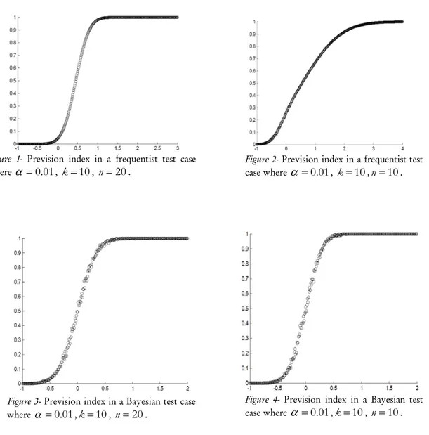
Are annexed below the curves representing the prediction of satisfaction according to the observation

x

. Simulation programs are written in MATLAB.

In each graph we take

σ

2

=

1

,

δ

=

0

and

τ

=

1

without loss of generality. We also choose to plot the curves

α

=

0.01

,

θ

₀

=

0

and

k =

10

. From one graph to the other varies the choice of

σ

₁2,

σ

₂2,

σ

₃2 ,

n

and the type of the test, frequentist or Bayesian. The curves are plotted with a

step of 0.01 for

x

and the following results are deduced for

n =

10

or

20

: TABLE 1 Variances table

10

n =

2 1

0.1

σ

=

2 2

0.1

σ

=

2 3

0.05

σ

=

20

n =

2 1

0.1

σ

=

2 2

0.05

σ

=

2 3

0.0333

σ

=

3.4.1. Index prediction in frequentist or Bayesian test

We wish to emphasize that the proposed predictive Bayesian approach can be used to predict results based on frequentist or Bayesian statements. We nevertheless believe that the frequentist approach provides a different insight on the data and should not be excluded. Prediction can be made as well for results derived from the frequentist approach as from the Bayesian approach. We present separately the numerical results to illustrate the achievement of original mathematical results with their pertinent application to the statistical analysis of real data.

Figures 1 and 2 represent the prevision curves in the case of a frequentist test study, we chose

50

N =

, and graphs 3 and 4 represent the prevision curves in the case of a Bayesian test study, recall that in this case our study is fully Bayesian and requires a larger number of simulations.

TABLE 2

Prevision index in a frequentist test for

N =

50

and

x =

0.5

.

10

k =

n =

20

π

( )

0.5

=

0.570

10

k =

n =

10

π

( )

0.5

=

0.421

TABLE 3

Prevision index in a Bayesian test for

N =

50

and

x =

0.5

.

10

k =

n =

20

π

_{( )}

0.5

=

0.926

10

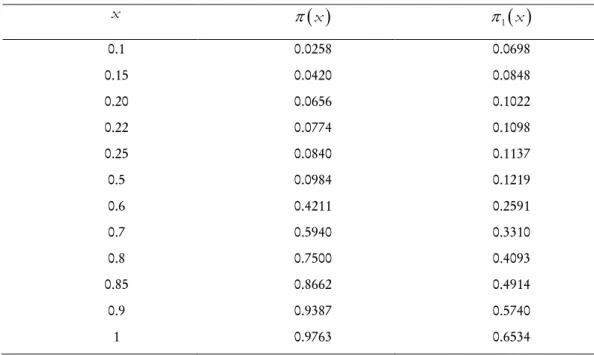
3.4.2. Comparison of prevision indices

If we denote by

π

₁

( )

_x

the prevision index in the case of experimental design, where inference involves an effect evaluated from only the future sample see (Merabet, 2004; 2004), figures 5 and 6 show compared curves

π

₁and

π

of the prevision indices in a study of frequentist test respectively in experimental design and in sequential analysis.

Figure 1- Prevision index in a frequentist test case where

α

=

0

.

01

,

k

=

10

,

n

=

20

.

Figure 2- Prevision index in a frequentist test case where

α

=

0

.

01

,

k

=

10

,

n

=

10

.

Figure 3- Prevision index in a Bayesian test case where

α

=

0

.

01

,

k

=

10

,

n

=

20

.

Figure 4- Prevision index in a Bayesian test case where

α

=

0

.

01

,

k

=

10

,

n

=

10

.

Note the consideration of all the information accumulated in the satisfaction index is more informative than

x

, the result of the first stage is large.

Some values are compiled in the following table where

k =

10

,

n =

20

and

N =

50

.

TABLE 4

Prevision indexes in experimental design and in sequential analysis for

k =

10

,

n =

20

and

N =

50

.

x

π

_{( )}

_x

π

1

( )

x

0.1 0.0258 0.0698 0.15 0.0420 0.0848 0.20 0.0656 0.1022 0.22 0.0774 0.1098 0.25 0.0840 0.1137 0.5 0.0984 0.1219 0.6 0.4211 0.2591 0.7 0.5940 0.3310 0.8 0.7500 0.4093 0.85 0.8662 0.4914 0.9 0.9387 0.5740 1 0.9763 0.6534 -1 -0.5 0 0.5 1 1.5 2 2.5 3 0 0.1 0.2 0.3 0.4 0.5 0.6 0.7 0.8 0.9 1

Figure 5- Prevision index

π

₁=··; Prevision index

π

=××, where

α

=

0

.

01

,

k

=

10

,

n

=

20

. -1 -0.5 0 0.5 1 1.5 2 2.5 3 0 0.1 0.2 0.3 0.4 0.5 0.6 0.7 0.8 0.9 1

Figure 6- Prevision index

π

₁=··; Prevision index

4. CONCLUSION

This work provides a fully Bayesian solution that incorporates the prevision in a global issue. In an interim analysis the predictive inference focuses on all data, the data available and future data. In this way the evaluation of the prevision error is not overvalued as in an approach that takes into account the future observation. The corresponding calculations of prediction are feasible by Monte Carlo methods. The numerical applications and simulation results in the Gaussian model illustrate the innovative methodology and provide the practitioner with tools ready to use.

In brief, this is an extremely useful work for clinical trials statisticians wishing to stay abreast with the innovative approaches that are being developed amid some controversies regarding their benefits. We believe it provides a valuable contribution to the area of design of sequential clinical trials.

ACKNOWLEDGEMENTS

I absolutely would like to thank Mr. Christian Robert, Professor at the University Paris Dauphine and Crest, Paris, for his help and advice on the organization and presentation of this work, I thank too the anonymous referees for several suggestions that have improved the presentation of this paper.

REFERENCES

S.M.BERRY,B.P.CARLIN,J.J.LEE,P.MULLER (2011). Bayesian Adaptive Methods for Clinical

Trials. Chapman & Hall/CRC biostatistics series.

B.W.BROWN,J.HERSON,N.ATKINSON And M.E.ROZELL (1987). Projection from previous studies:

A Bayesian and frequentist compromise. Controlled Clinical Trials, 8, pp. 29-44.

S. C. CHOI, P. A. PEPPLE (1989). Monitoring clinical trials based on predictive probability of

significance. Biometrics, 45, pp. 317-3231.

S.C.CHOI,M.CHANG (2011). Adaptative Design Methods in clinical trials. Chapman & Hall/CRC. Biostatistics series.

A. GIOVAGNOLI, M. ZAGORAIOU (2012). Simulation of Clinical Trials: A Review with Emphasis on

the Design Issues. Statistica, Volume 72, Issue 1, pp. 63-80.

A.P.GRIEVE (1992). Predictive probability in clinical trials. Biometrics, 41, pp. 979-990.

J.M.GROUIN (1994). Procédures bayésiennes prédictives pour les essais expérimentaux, thèse de doctorat

de l'Université René Descartes. Paris.

E.HOLST ,P.THYREGOD,PETER-TH.WILRICH (2001). On conformity testing and the use of two stages procedures. International Statistical Review, 69, 3, pp. 419-432.

accuracy in testing. Ann. Statist., 1, pp. 490-509.

C.JENNISON, B.W.TURNBULL (2000). Group Sequential Method with Applications to Clinical Trials.

Chapman and Hall/CRC Press, New York.

B.LECOUTRE,G.DERZKO,J.M.GROUIN (1995). Bayesian predictive approach for inference about

proportions. Statistics in Medicine, 14, pp. 1057-1063.

H.MERABET,J.P.RAOULT (1995). Les indices de satisfaction, outils classiques et bayésiens pour la prédiction statistique. ASU, XXVIIèmes Journées de Statistique, Jouy-en-Josas.

H.MERABET (2004). Méthodologie des essais préliminaires. Calcul de prévision de satisfaction dans le

cas Gaussien. Rev. Statistique Appliquée, LII (3), pp. 93-106.

H. MERABET (2004). Index and prevision of satisfaction in exponential models for clinical trials. Statistica. anno LXIV, 3, pp. 441-453.

P.MULLER,D.A.BERRY,A.P.GRIEVE,M.KRAMS (2006). A Bayesian decision-theoretic-dose finding trial. Decision analysis, 3, 4, pp. 197-207.

C.P.ROBERT,G.CASELLA (2004). Monte-Carlo Statistical Methods. 2nd Edition, Springer-Verlag. A. O'HAGAN, J.W. STEVENS, M.J. CAMPBELL (2005). Assurance in clinical trial design.

Pharmaceutical Statistics, 4, pp. 187-201.

C.P.ROBERT (2006). Le choix Bayésien. Springer, Paris.

G.YIN,N.CHEN,J.J.LEE (2012). Phase II trial design with Bayesian adaptive randomization and

predictive probability. Journal of the Royal Statistical Soc, Volume 61, Issue 2, pp. 219-235.

SUMMARY

Bayesian sequential analysis of clinical trials feedback

The paper deals with the Bayesian sequential analysis of clinical trials and the related predictive approach in a particularly innovative fashion. We propose a unified methodology for sequential clinical trials under a Bayesian paradigm. The idea is to make predictive inference based on the data accrued so far together with future data. We apply a prevision based approach to Gaussian data and end up with some numerical illustrations.