View of Some recent developments in the design of adaptive clinical trials

SOME RECENT DEVELOPMENTS IN THE DESIGN OF ADAPTIVE CLINICAL TRIALS

A. Baldi Antognini, A. Giovagnoli, M. Zagoraiou

1. INTRODUCTION

Most clinical trials are carried out to compare different drugs or therapies. Pharmaceutical industries in particular invest very large budgets for research and development of new drugs but recently the increased spending in biomedical re-search has not reflected in a corresponding increase in benefits. Furthermore, in a clinical trial the ethical concern of assigning treatments to patients so as to care for each of them individually often conflicts with the experimental demands. To overcome this impasse, the FDA Critical Path initiative of 2004 supports and en-courages innovative approaches in the design of the trial, in particular the use of adaptive designs. Adaptive designs are sequential procedures that use the available information at each stage to modify aspects of the trial without undermining its validity and integrity. Special cases are

i) group sequential designs for early termination of the trial due to efficacy or futility through interim analyses;

ii) sample size re-estimation designs;

iii) adaptive dose-finding designs to minimize toxicity while acquiring informa-tion on the maximum tolerated dose;

iv) covariate-adjusted designs;

v) adaptive randomization designs for treatment comparison with the ethical aim of skewing allocations towards the best treatment or dropping the less suc-cessful treatment arms.

The past decade has witnessed an outburst of books and papers on the topic of adaptive designs in clinical trials, see for instance Chow and Chang (2007), which pertain mainly to the medical and pharmaceutical literature. At the same time, the topic has aroused a wide interest among statisticians with a more atten-tive eye to the methodological implications, see for instance the book by Hu and Rosenberger (2006).

In two recent papers (Baldi Antognini and Giovagnoli, 2010; Baldi Antognini and Zagoraiou, 2010) the present authors have looked at designs of type v) ap-proaching the ethical design problem of individual vs collective ethics via the

op-timization of specific compromise criteria given by a weighted average of a design optimality measure and a measure of the subjects’ risk. The relative weights in the compound criterion have been allowed to depend on the true state of nature, since it is reasonable to suppose that the more the effects of the treatments differ, the more important for the patients are the chances of receiving the best treat-ment. The purpose of the present paper is to extend the theoretical results ob-tained in Baldi Antognini and Giovagnoli (2010) and Baldi Antognini and Zagoraiou (2010) and enhance their applicability by including some numerical ex-amples. For simplicity we consider just two treatments, as is usually the case in Phase III trials, where the aim may be either to estimate the treatment effects separately or, more commonly, to estimate or test their difference.

We shall first of all find the target allocation that optimizes a given compound criterion for different response models and different choices of the optimality measures. This target in general depends on the unknown parameters, and we will present adaptive randomization methods that make the experiment converge to the desired target, whatever the true value of the parameters, extending the dou-bly-adaptive biased coin design of Hu and Zhang (2004). The last part of the pa-per discusses a special case of adaptive randomization when one categorical co-variate is also observed.

We end this introduction by pointing out that for binary responses, a popular design with an ethical slant is the so-called Play-the-Winner proposed by Zelen (1969) and later extended to include randomization (Ivanova, 2003; Wei and Durham, 1978). Play-the-Winner is a sequential experiment in which the treat-ment allocation is repeated for the next patient in case of success, or switched to the other arm in case of failure. It is widely believed to be “an optimal model that minimizes the number of failures” (Chow and Chang, 2007), but this claim is not justified by the theory. It can be shown however that when the number of obser-vations goes to infinity the limit allocation of each treatment is inversely propor-tional to the treatment risk, which clearly always favours the better treatment.

2. THE COMPOUND CRITERION AND THE OPTIMAL ALLOCATION 2.1. The model

Given two treatments T and 1 T with n subjects recruited into the trial, let 2,

ik

Y be the response of patient (i i1,..., )n to treatment T (k k 1, 2).

Condi-tionally on the treatment assignment, the responses are usually taken to be inde-pendent. Put

2

E(Y_ik)_k, Var(Y_ik)_k (1)

and assume a “the-larger-the--the better scenario”. Special cases are 1) homoscedastic responses, i.e. 2 2

1 2

2) when the responses are binary, with p , 1 p being the respective success 2 probabilities:

E(Yik) Pr( Yik  1) pk, Var(Yik) p qk k (2)

and q_k  1 p_k.

We may further assume the dependence of p or k k on some patient-related

covariates.

After n subjects are assigned to ₁ T and ₁ n₂  to n n₁ T , let ₂  and 1 be  the proportions of allocations to T and 1 T respectively. The ML estimators of 2

1

 and 2 in general are the sample means and their variance-covariance matrix (exact or asymptotic) is proportional to

2 1 2 2 0 . 0 1 V               _   

2.2. The treatment allocation

We shall refer to all the desirable treatment allocations as “targets”. In Optimal Design Theory, the design problem consists in minimizing a suitably chosen op-timality criterion _I, which measures the loss of potential information ensuing from the experimental design. In particular, the D -optimality criterion det( )V

measures the global variance and the trace criterion tr( )V measures the variance

of the estimated difference 12; under suitable assumptions it also measures the power of Wald’s test of the equality of treatment effects. In this setting, popu-lar treatment allocation schemes are the balanced one, _B _1/2_{, which} mini-mizes det( )V , and the well-known Neyman allocation

1 1 2 , N      _  (3) which minimizes tr( )V .

From an ethical viewpoint one possible “optimality criterion” is the proportion

W

 of patients who receive the worse treatment,

1 2 1 1 (1 2 )sgn( ) 2 2 W        

which would be minimized, trivially, by assigning all the patients to the better treatment, if we knew which one this is. This choice however would make the treatment comparison impossible.

In practice, we would most likely wish to simultaneously minimize both the ethical cost and the inferential loss. Note that both are functions of  . A possi-bility is to measure the trade-off by means of some compromise function, such as a weighted average of I and W , suitably standardized to make them

compa-rable (see for instance Baldi Antognini and Giovagnoli, 2010). One way is to set min ( ) 1 ( ) I I I             

so that both functionals W and I range in [0,1) , with 0 being their best

value.

We can look at the combination (1 )

W I

  

      (4)

as the compound criterion to be minimized. We can attempt to find the optimum allocation  arg min by differentiation of  wrt  , i.e. look for a solu-tion in (0,1) of 1 2 sgn( ) 1 0 (1 ) _{I I}                _{ }  _{ } (5)

where _I min_I. The target  will in general depend on the following:  the inferential criterion _I. As already pointed out, either D -optimality or

trace-optimality will in general be chosen as I;

 the weight  chosen by the experimenter, with 0  It may be fixed or  1. function of some or all the unknown parameters. The choice of the best weight function ( )  in a given applied context is open to discussion, but here are some general remarks:

1) the function  should deal with T and 1 T symmetrically; 2

2)  should be non-decreasing in the absolute difference of the treatment ef-fects, to make the ethical impact more crucial the more the effects differ, whereas, on the other hand, a small difference is more difficult to detect correctly, so more emphasis is needed on precision (i.e. small )

 The unknown parameters. The dependence of the target on the unknown pa-rameters may appear like an unsolvable puzzle, in this as well as in other cases, as for instance the classical Neyman allocation (3). We shall deal with this problem in Section 5.

3. OPTIMAL TARGETS

3.1. The compound target when I is D-optimality

We assume model (1) and _I det( )V . Equation (5) becomes

1 2 2 2 2 2 1 2 1 2 sgn( ) (1 ) (1 ) 4                    _{ }  _{ } (6) and 1 2 1 1 1 sgn( )min , . 2 8 1 2        _{  }      _{ } _    (7)

is the optimum target. The expression for  is independent of ( 12, 22). If 4/5  then 1 2 1 1 sgn( ) (0,1); 2 8 1        _{  }   _  _    (8)

otherwise, if 4/5,  will assign all the subjects to the better treatment. For binary responses, the optimum target will clearly be

1 2 1 1 1 sgn( )min , . 2 p p 8 1 2      _{  }       _      

It is evident that the target allocation (7) will always assign more than half the subjects to the better treatment.

3.1.1 The choice of the weights

We can define the “ethical gain” in terms of relative percentage of fewer sub-jects assigned by  to the worse treatment than by the balanced design, namely when   . Assuming (wlog) 0 12, it is easy to find the expression of the ethical gain: 1 8 1( ) (1 ) (1 ) 1 . 1/ 2 4 1 1 B B                _{  }       (9)

We can measure the inferential loss by 2 min det( ) 1 1 . det( ) 16 1 D V V       _ _    (10)

The ethical gain and the inferential loss for the optimal compound target defined in (8) are compared in Table 1.

The percentual ethical gain of the compound target is always greater than the percentual inferential loss, with maximum difference at 1/2.

Another possibility is to let the weight  depend on the parameters. Example 1 (Normal case) For normal responses we could choose

1 2 2 2 1 2 4 1 , 5 e              _  _     (11)

so that   (0,1) is satisfied. Letting 12 (wlog), Table 2 shows possible values of

2 2

1 2 1 2

(  )/   and the corresponding values of the compound target:

TABLE 1

The relative ethical gain and the relative inferential loss for target

  _{in (8) as ω varies when μ} 1>μ2 ω  % ethical gain _{4(1 )}    % inferential loss 2 4(1 )      _    0.00 0.50 0.00 0.00 0.10 0.51 2.78 0.08 0.20 0.53 6.25 0.39 0.30 0.55 10.71 1.15 0.40 0.58 16.67 2.78 0.50 0.63 25.00 6.25 0.60 0.69 37.50 14.06 0.70 0.79 58.33 30.03 0.75 0.88 75.00 56.26 TABLE 2

Values of the optimum compound target allocation



 _{in (8) with ethical weight}

1 2 2 2 1 2 4 ₁ 5 e              _  _     1 2 2 2 1 2       ω  → 0 → 0 0.500 0.25 0.18 0.527 0.50 0.31 0.557 0.75 0.42 0.591 1.00 0.51 0.628 1.50 0.62 0.705 3.00 0.76 0.896 → ∞ → 0.8 1.000

Example 2 (Binary case) For binary responses a possible choice of the weight function

is the one suggested in Baldi Antognini and Giovagnoli (2010), namely 2

1 2 1 2

( ,p p ) {(p p ) 1}/ 2

    , but the condition 4/5 is not always satisfied.

An-other choice is 1 2 1 2 4 ( , ) | |. 5 p p p p    (12)

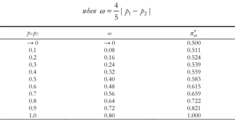
Table 3 gives the target allocation to the better treatment as a function of the difference in success probabilities.

TABLE 3

Values of the target as a function of the difference in success probabilities

when 4| 1 2| 5 p p   p1-p2 ω  → 0 → 0 0.500 0.1 0.08 0.511 0.2 0.16 0.524 0.3 0.24 0.539 0.4 0.32 0.559 0.5 0.40 0.583 0.6 0.48 0.615 0.7 0.56 0.659 0.8 0.64 0.722 0.9 0.72 0.821 1.0 0.80 1.000

3.2. The compound target when _I is trace-optimality

Since 2 2 1 2 tr( )V  /  /(1) and 2 1 2 min tr( ) (V    ) , equation (5) becomes 1 2 2 2 2 1 2 2 1 sgn( ) (1 ) 0. 1 ( ) ( ) 1                     _{ }   _   _ (13) When 2 2 1 2

  , equation (13) is identical to (6), so that all the results of Sub-section 3.1 apply. Let now 2 2

1 2

  ; (13) can be rewritten as a quadratic equation in  : 2 2 2 1 2 2 1 2 2 2 2 2 2 1 2 2 1 1 1 sgn( )[( ) 1] 1 ( ) [( ) 2 ] 0.                           (14) If the solution

2 2 2 1 2 1 2 1 2 1 1 2 1 1 1 1 sgn( ) 1  _                                (15)

lies in (0,1) , it will give the optimum allocation to T as a function of 1 ,  2/ 1 and sgn(12). The LHS of (14) is monotonic in [0,1], so the existence of a unique solution in (0,1) is ensured if the LHS is negative at 0 and positive at 1 namely if 2 2 1 2 1 2 2 1 1 sgn( ) 1 , 1              _{ }    _  _     

which holds if and only if 2 1 2 2 2 1 2 ( ) _. 1 max( , )          (16)

We may be able to use some previous knowledge on 2 1

 and 2 2

 in order to choose a weight function that satisfies (16). Since 1 2

1 2 max( , )

1  _{ }  , again 2 4/5 will have to hold true. The condition 1/2, which means that the ethical im-pact should not prevail over the inferential goal, is enough to guarantee (16) for all 2

1

 and 2 2

 , but at times may be too restrictive.

Table 4 shows the optimal targets  given by (15) for different values of the ratio  2/ 1 and different choices of /(1 ), compared with the Neyman al-location.

The top and the bottom parts of Table 4 show the unfavourable cases, i.e.

1 2

  with  12 or 12 with 12, in which Neyman’s allocation is unethical, namely it assigns more patients to the worse treatment. The optimal compound target counteracts this effect, especially with a large . This points to the need for adaptive weights, for instance by choosing (11) as the weight func-tion. However, Table 4 seems to suggest that the weight  perhaps should de-pend also on  2/ 1.

Remark In this case, whether or not the optimal compound target assigns more than half the

subjects to the better treatment depends on the weights and the true values of the parameters. However, there is always an ethical gain, in terms of more subjects assigned by the target  to the better treatment than by the inferentially optimum Neyman target N . To show this, it is sufficient to check that sgn(12) sgn(  N), replacing  by (15).

TABLE 4

Optimal target  for different values of 2/1 and ω/(1-ω)

when ΨI is the trace, compared with Neyman’s N

1    2 1   0.20 0.33 0.50 1.00 1.50 2.00 3.00 * N  μ1> μ2 5.00 0.18 0.19 0.21 0.32 1.00 1.00 1.00 0.17 4.00 0.22 0.23 0.25 0.35 0.78 1.00 1.00 0.20 2.00 0.36 0.37 0.40 0.48 0.61 0.82 1.00 0.33 1.50 0.42 0.44 0.46 0.54 0.63 0.75 1.00 0.40 1.33 0.45 0.47 0.49 0.57 0.65 0.74 0.98 0.43 1.00 0.52 0.54 0.56 0.63 0.69 0.75 0.88 0.50 0.80 0.58 0.60 0.61 0.67 0.72 0.77 0.85 0.56 0.50 0.69 0.70 0.72 0.76 0.79 0.82 0.86 0.67 0.33 0.79 0.80 0.81 0.83 0.85 0.87 0.90 0.77 0.25 0.81 0.82 0.83 0.86 0.87 0.89 0.91 0.80 0.20 0.85 0.85 0.86 0.88 0.89 0.91 0.92 0.83 μ1< μ2 5.00 0.15 0.15 0.14 0.12 0.11 0.09 0.08 0.17 4.00 0.19 0.18 0.17 0.14 0.13 0.11 0.09 0.20 2.00 0.31 0.30 0.28 0.24 0.21 0.18 0.14 0.33 1.50 0.38 0.36 0.34 0.30 0.25 0.21 0.15 0.40 1.33 0.41 0.39 0.37 0.32 0.27 0.23 0.15 0.43 1.00 0.48 0.46 0.44 0.37 0.31 0.25 0.12 0.50 0.80 0.53 0.51 0.49 0.42 0.34 0.26 0.06 0.56 0.50 0.64 0.63 0.60 0.52 0.39 0.18 0.00 0.67 0.33 0.75 0.74 0.71 0.61 0.35 0.00 0.00 0.77 0.25 0.78 0.77 0.75 0.65 0.22 0.00 0.00 0.80 0.20 0.82 0.81 0.79 0.68 0.00 0.00 0.00 0.83

Assuming 1 (wlog), the ethical gain is given by 2

1 N N         

and the loss of efficiency is

2 tr 1 2 2 2 2 2 1 1 (1 ) min tr( ) 1 1 ( ) . tr( ) ( ) V V                       

For the binary model (2), equation (14) becomes 2 2 2 1 2 1 1 2 2 2 2 2 2 1 1 1 1 sgn( ) 1 1 1 1 1 2 1 0 p q p p p q p q p q p q p q           _  _  _   _{  }                  _{   }     (17)

and condition (16) translates to 2 1 1 2 2 1 1 2 2 ( ) . 1 max( , ) p q p q p q p q      (18)

When p₁p₂, the unfavourable case occurs if p q_{1 1} p q_{2 2}. In Table 5 we show the optimum compound targets that correspond to different choices of the weight ratio /(1 ) and different values of p , 1 p , and compare them with 2 the Neyman allocation N and the Play-the-Winner target PW 2

1 2 . q q q  _ TABLE 5

Optimal target  for different values of p1, p2 and ω/(1-ω) when ΨI is the trace, compared with Neyman’s N

and the Play-the-Winner target pW

ω/(1-ω) p1 p2 0.05 0.11 0.25 1.00 1.50 2.00 2.50 3.00  *N *pW 0.10 0.05 0.586 0.593 0.609 0.688 0.735 0.777 0.816 0.851 0.579 0.514 0.20 0.05 0.653 0.660 0.674 0.741 0.777 0.808 0.834 0.858 0.647 0.543 0.20 0.10 0.578 0.585 0.601 0.682 0.730 0.774 0.814 0.851 0.571 0.529 0.40 0.05 0.698 0.704 0.717 0.775 0.805 0.830 0.851 0.869 0.692 0.613 0.40 0.20 0.557 0.564 0.581 0.666 0.717 0.766 0.811 0.854 0.551 0.571 0.40 0.35 0.513 0.521 0.538 0.630 0.691 0.752 0.812 0.871 0.507 0.520 0.65 0.40 0.500 0.507 0.525 0.620 0.684 0.748 0.814 0.880 0.493 0.632 0.65 0.60 0.500 0.507 0.525 0.620 0.684 0.748 0.814 0.880 0.493 0.533 0.95 0.65 0.319 0.326 0.343 0.465 0.606 0.881 1.000 1.000 0.314 0.875 0.95 0.85 0.385 0.392 0.410 0.524 0.625 0.760 0.954 1.000 0.379 0.750

Although PW always assigns more than half the subjects to the better

treat-ment, the PW target assignment would perform poorly for inference.

4. DIFFERENT CRITERIA FOR THE BINARY MODEL 4.1. Changing the measure of ethical loss

For binary responses, another possible measure of ethical loss is the expected proportion of failures:

1 2 1 1 2 2

( , ) ,

F

E    q  q

which is related to W by a linear transformation:

min 1 1 1 2 min max min 1 2 1 1 2 (1 ) | | 1 1 _{sgn( ) .} 2 2 F W E q q q q q q p p p p      _         _  _    

If we minimize the compound criterion ( 1) (1 ) , F I E        

this is equivalent to minimizing criterion (4) with different weights. More pre-cisely,

[ 0,1] [ 0,1]

1 2

1 2

arg min [ (1 ) ] arg min [ (1 ) ]

| | where | | 1 F I W I E p p p p                           

Basically, we are re-scaling the weight ratio, namely _1_|p1p2|_{1 . The} _ results of Sections 3.1 and 3.2 can be applied after suitable changes. In particular,  for the determinant: the choice 4/5 ensures 4/5 and in this case the

optimal target is 1 2 1 1 ( ) ; 2 p p 8 1      _{  }  (19)

 for the trace: replace ₁_{ by  1}_|p1 p2| in equation (14) and replace condition (18) by 2 1 1 2 2 1 2 1 1 2 2 ( ) | | . 1 max( , ) p q p q p p p q p q       

4.2. Changing the compound criterion

Now we want to deal with an altogether different compound criterion, the one that was assumed in Baldi Antognini and Giovagnoli (2010), namely:

( 2 ) 1 2 1 2 1 2 ( , ) ( , ) ( , ) (1 ) . min min F I F I E E                  _{ }  _{ }     (20)

Since the minimum value of E is simply _F q_min, by differentiation the defining equation of this new compound target is

1 2 min ( ) 1 (1 ) I 0. I p p q             (21)

4.3. The targets wrt criterion (20)

If _I  -optimality, equation (21) becomes D

1 2 1 1 2 2 1 1 2 2 min 4 0, 1 (1 ) p p p q p q p q p q q             _{ }  _  _

i.e. 1 2 2 2 min 4( ) 2 1 0, 1 (1 ) p p q             (22)

and the optimal target is obtained by solving (22) in (0,1) . Since the LHS of (22) is monotonic and as   and 1, the limits are  and  , respectively, there 0 is a unique solution in (0,1) . The important difference from considering criterion (4) is that in this case the optimal solution depends on the actual values of p p₁, ₂ and not just on the sign of their difference.

Remark It is evident from (22) that this target will always assign more than half the subjects

to the better treatment, since sgn(2 1) sgn(p1 p2). If _I trace-optimality, the defining equation is

2 1 2 1 1 2 2 1 1 2 2 min ( ) 0 (1 ) 1 p p p q p q p q p q q         _{ }  _ _       namely





Remark It is shown in Baldi Antognini and Giovagnoli (2010), that with this target

alloca-tion, the majority of subjects will receive the better treatment if the weight function is chosen so that ( , ) 1/2 x y  when x  . y 1

Table 6 shows the values of the compound targets that solve (22) and (23), corresponding to fixed weight 1/2 (1/2 and 1/2, respectively) and to

1 2

( p p 1)/2

   (_p and p



, respectively) for several choices of p and 1 2

p .

TABLE 6

Values of the compound targets for D- and trace-optimality, corresponding to ω=1/2 and ωp=(|p1-p2|+1)/2,

for different choices of p1 and p2

D-optimality trace-optimality p1 p2 1/ 2 p  ** 1/ 2    **p N pW 0.10 0.05 0.507 0.508 0.586 0.587 0.579 0.514 0.20 0.05 0.523 0.531 0.668 0.675 0.647 0.543 0.20 0.10 0.516 0.519 0.587 0.590 0.571 0.529 0.40 0.05 0.570 0.631 0.744 0.782 0.692 0.613 0.40 0.20 0.541 0.561 0.590 0.609 0.551 0.571 0.40 0.35 0.510 0.512 0.517 0.518 0.507 0.520 0.65 0.40 0.584 0.630 0.578 0.624 0.493 0.632 0.65 0.60 0.518 0.520 0.511 0.513 0.493 0.533 0.95 0.65 0.802 0.852 0.724 0.796 0.314 0.875 0.95 0.85 0.686 0.709 0.599 0.629 0.379 0.750

The targets 1/2 and p



assign more patients to the better treatment, whereas the bottom part of Table 6 (outlined) shows the values of ( ,p p for 1 2) which the Neyman target penalizes the better treatment. Clearly the values of

1/2  

 and _p, and of 1/2 and _p are very close when |p1 p2| is small.

5. CONVERGENCE TO THE OPTIMAL ALLOCATION: RESPONSE-ADAPTIVE EXPERIMENTS As shown previously, the target allocation depends in general on some or all the unknown parameters of the model, e.g.   ( ) with { ,   1 12; ,2 22}, and when this function is continuous response-adaptive procedures may be called for. These designs, also called response-driven or data-dependent, use the observed responses as well as past allocations to modify the experiment as we go along in order to gradually approach the desired target allocation.

Now we briefly describe the general framework of these sequential methods. Starting with n observations on each treatment, usually assigned by using re-0 stricted randomization, e.g. permuted block designs, an initial non-trivial parame-ter estimation  is derived. Then, at each step n (ˆ0 n2 )n0 let ˆ( )n be a consis-tent parameter estimator of  based on the first n observations, so that the op-timal target will be estimated by all the data up to that step. Let ˆ( )n  ( ( ))ˆ n .

Moreover, let N n and ₁( ) N n be the number of patients assigned to ₂( ) T and ₁ 2

T , respectively, with N n1( )N n2( ) ; additionally, n ( )n n N n1 1( ) is the random proportion of allocation to T and, symmetrically, 11 ( )n to T . When 2 patient (n  is ready to be randomized, s/he will be assigned to 1) T with prob-1 ability Pn1 (consequently, to T with probability 2 1Pn1) and the problem con-sists in choosing the allocation probabilities { ,P n  so that, as n tends to in-_n 1} finity, ( ) n converges to  ( ) in some sense.

One of the most effective family of randomization procedures is the Doubly Adaptive Biased Coin Design (D-BCD) analyzed by Hu and Zhang (2004) (see also references therein). The rationale behind this procedure consists in favouring the allocation of a given treatment, the more so the more its current allocation proportion is smaller than the current estimate of the target. The D-BCD consists in assigning treatment T to subject (1 n  with probability 1)

1 ( ( ); ˆ ( ))

n

P  g  n  n for all n2n0, where the allocation function ( ; )g   is cho-sen by the experimenter so as to force the treatment assignments on the basis of some measure of the dissimilarity between their actual allocation proportion x and the current estimate of the optimal target y . The function g needs to satisfy the following conditions:

i) g x y is continuous on (0,1)( ; ) 2_; ii) g x x( ; ) ; x

iii) ( ; )g x y is decreasing in x and increasing in y ;

iv) ( ; ) 1g x y  g(1x;1 y) for all x, y  (0,1)2

Observe that the D-BCD will force the allocation proportion to the target, since from conditions ii) and iii), when x y then ( ; )g x y < y, whereas if x y, then ( ; )g x y >y. However, condition i) is quite restrictive since it does not include

several widely-known procedures based on discontinuous allocation functions such as Efron’s Biased coin design and its extensions (Hu et al. 2009), while con-dition iv) simply guarantees that T and 1 T are treated symmetrically. 2

The following result ensures the convergence of the D-BCD to the chosen compound optimal target allocation  ( ) (see for instance Hu and Zhang, 2004):

Proposition If the compound optimal target  ( ) (0,1) and is continuous in ,

adopting the D-BCD

ˆ

lim ( ) ( ) and lim ( ) . .

n  n   n  n  a s



   

Now we give some examples belonging to the D-BCD family:

Method 1. The most “intuitive” allocation rule consists in letting g x y( ; ) ; y

this means that treatment T will be assigned to subject 1 n  with probability 1

1 ˆ ( ).

n

P  n (24)

When estimation is made by ML, this procedure is called the Sequential Maxi-mum Likelihood (SML) or recursive MaxiMaxi-mum Likelihood design. See Baldi An-tognini and Giovagnoli (2005) and references therein.

Method 2. Hu and Zhang (2004) suggest the following family of allocation func-tions ( / ) ( ; ) , ( / ) (1 )[(1 )/(1 )] y y x g x y y y x y y x     _{   }  (25)

where the non-negative parameter  controls the degree of randomness of each allocation: if  0 the randomization function does not dependent on the cur-rent allocation proportion and this procedure corresponds to the SML design in (SML), whereas as  grows the allocation tends to be forced deterministically to the estimated target.

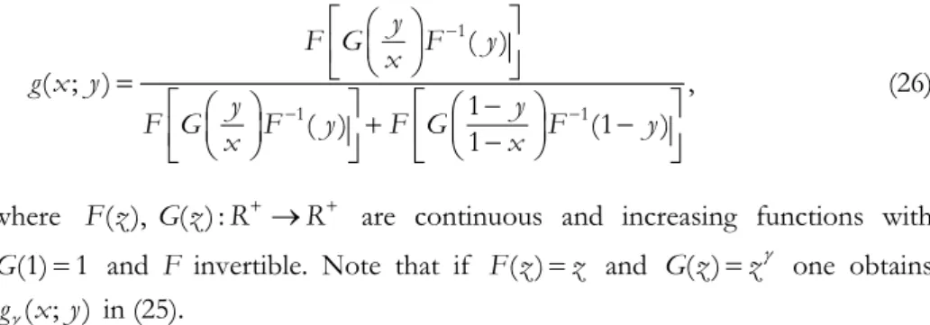
Method 3. A new proposal of allocation function is: 1 1 1 ( ) ( ; ) , 1 ( ) ₁ (1 ) y F G _x F y g x y y y F G _x F y F G _x F y           _{ }         _    _       _{ }   _{  }      (26)

where F z G z R( ), ( ) : R are continuous and increasing functions with (1) 1

G  and F invertible. Note that if ( )F z  and ( )z G z  one obtains z

( ; )

g x y in (25).

Example 3 Set ( )G z  . We let z

1 1 1 ( ) ( ; ) , 1 ( ) ₁ (1 ) y F _x F y g x y y y F _x F y F _xF y             _  _     _       ₍₂₇₎ where ( ) 2 0 2 z t F z e dt  

 _ (this F is called the error function).

Figure 1 shows the behaviour of the function g in (27).

Fig. 1 – Plots of ( ; )g x y as x varies in (0,1). The values of y from the bottom curve to the top curve

are: 0.2, 0.4, 0.6 and 0.8, respectively.

Table 7 shows the comparisons between the above mentioned randomization functions, i.e. Method 1, Method 2 and Method 3, in order to stress the different impact of these procedures in terms of treatment allocations when both the target estimate and the allocation proportion vary.

The SML design (Method 1) is not affected by the current allocation propor-tions but depends only on the current estimate of the target. As an example, when y 0.7 the SML design favours the allocation of T by assigning 1 T with 1 probability 0.7 , both in case of x 0.05 and x 0.8. Method 2, however, strongly depends on the current allocation proportion. Indeed, the top part of Table 7 shows that if treatment T has (almost) never been assigned, then it will 1 be allocated with probability 1 even if the target allocation is extremely small (e.g.

0.1

y  or y 0.3). Furthermore, starting from  2 Method 2 tends to be highly deterministic. On the contrary, the proposed g in (27) has an interesting behaviour as regards the drawbacks of Methods 1 and 2, since it forces the alloca-tion decisively onto the target, when needed, guaranteeing at the same time a suit-able degree of randomness.

TABLE 7

Values of the randomization function g in (25) with =0, namely the SML design,  =1,  =2 and g in (27)

x y g0(SML) g1 g2 g → 0 0.1 0.1 1.000 1.000 0.537 → 0 0.3 0.3 1.000 1.000 0.653 → 0 0.5 0.5 1.000 1.000 0.792 → 0 0.7 0.7 1.000 1.000 0.916 → 0 0.9 0.9 1.000 1.000 0.990 0.2 0.1 0.1 0.047 0.022 0.051 0.2 0.3 0.3 0.424 0.557 0.407 0.2 0.5 0.5 0.800 0.941 0.735 0.2 0.7 0.7 0.956 0.995 0.897 0.2 0.9 0.9 0.997 0.999 0.988 0.4 0.1 0.1 0.018 0.003 0.025 0.4 0.3 0.3 0.216 0.151 0.227 0.4 0.5 0.5 0.600 0.692 0.585 0.4 0.7 0.7 0.891 0.966 0.859 0.4 0.9 0.9 0.992 0.999 0.984 0.6 0.1 0.1 0.008 0.001 0.016 0.6 0.3 0.3 0.109 0.034 0.141 0.6 0.5 0.5 0.400 0.308 0.415 0.6 0.7 0.7 0.784 0.850 0.773 0.6 0.9 0.9 0.982 0.997 0.975 0.8 0.1 0.1 0.003  0 0.012 0.8 0.3 0.3 0.044 0.005 0.103 0.8 0.5 0.5 0.200 0.059 0.265 0.8 0.7 0.7 0.577 0.443 0.593 0.8 0.9 0.9 0.953 0.979 0.949

6. THE HOMOSCEDASTIC MODEL WITH ONE CATEGORICAL COVARIATE We now further specify (1) as follows

2

( ik) k it , ( )i 1, 2,...,

E Y  z  V Y  i n (28)

namely the observations are homoscedastic and the response depends on the treatment and on one random categorical covariate Z with J fixed levels. The subjects will be subdivided into strata (blocks) according to the level of Z . This

case was dealt with in Baldi Antognini and Zagoraiou (2010). The covariate dis-tribution in the population is assumed to be known: _j Pr(Z z _j) for

1,...,

j J;  is the vector of block effects and z is the indicator function of i

the block for the i th observation. Conditionally on the covariate and the treat-ment allocations, patients’ responses are assumed to be independent. In the statis-tical literature (28) is described as a 2-factor mixed model without treatment-block interaction; in other words, the superiority of one treatment over the other (meaning 1 or vice-versa) is uniformly constant over the blocks. The inferen-2 tial interest typically lies in testing or estimating the difference 1 as precisely 2 as possible and  is usually a nuisance parameter.

Let N (j j 1,...,J) with Jj1Nj  be the random size of block n j after n

observations and let  ( ,...,1 J)t denote the vector of allocation proportions

to T in each block. Let 1 Z( ,...,Z1 Zn)t be the vector of covariates for the n

subjects. Then we obtain 1 2 2 1 2 1 ˆ ˆ ( | ) (2 1) , J j j j Var    n  N         _   _   



so the inferential loss depends on the design through the allocation vector  and the block sizes. The loss is a minimum if the treatments are equally replicated within each block (for a recent discussion see Baldi Antognini and Zagoraiou, 2011). The loss is random, since it depends on the block sizes which are not un-der the experimental control, therefore one must average over the covariate dis-tribution. After some suitable simplifications and approximations we can let our criterion be 1 2 2 1 1 ( ) J (2 1) J (2 1) I j j j j j j E n  N             





The percentage of patients assigned to the worse treatment is

1 2 1 1 1 ( ) sgn( ). 2 2 J W j j j        _  _  



We choose the compound criterion of Section 2, i.e. ( ) W( ) (1 ) ( ).I

  

Setting the partial derivatives with respect to  equal to 0 we find the set of j equations 1 2 sgn( ) 4(1 )(2 j 1) 0 for all j 1,..., .J            

Thus the same result as (7) applies to each block so that the optimal target 1 ( ,..., )t J      is given by 1 2 1 1 1

sgn( )min , for all 1,..., .

2 8 1 2 j j J        _{  }     _   _       (32)

Observe that the optimal compound target does not depend on the covariate probabilities j’s and if the weight function is chosen so that 4/5, then πωj*  (0,1). When J  (no covariates), then 1 1 2 12 and (32) reduces to expression (7).

Remark This allocation is always “ethical”, i.e. more subjects are assigned to the better treat-ment, whatever their covariate value. Since the compound optimal allocations in all the blocks are the same as (7), there is no need for further examples.

The optimum  can be targeted by a suitable implementation of the above mentioned sequential methods adjusted for covariates by applying the same ran-domization function for each block. However, in Baldi Antognini and Zagoraiou (2010) a different method was employed namely the randomization function

( / ) ( ; ) ( / ) (1 )[(1 )/(1 )] j j j j y y x g x y y y x y y x         with 1 j j

 _ _{for all j 1,...,J , so the allocations for the profiles which may be} potentially under-represented will be forced towards the optimal target.

ACKNOWLEDGEMENTS

This research was partly supported by the Italian Ministry for Education, Uni-versity, and Research protocol 2007AYHZWC Statistical methods for learning in clinical research.

Department of Statistical Sciences ALESSANDRO BALDI ANTOGNINI

University of Bologna ALESSANDRA GIOVAGNOLI

REFERENCES

A. BALDI ANTOGNINI, A. GIOVAGNOLI (2005), On the large sample optimality of sequential designs for

comparing two or more treatments, “Sequential Analysis”, 24, pp. 205-217.

A. BALDI ANTOGNINI, A. GIOVAGNOLI (2010), Compound optimal allocation for individual and

collec-tive ethics in binary clinical trials, “Biometrika”, 97, pp. 935-946.

A. BALDI ANTOGNINI, M. ZAGORAIOU (2010), Covariate adjusted designs for combining efficiency, ethics

and randomness in normal response trials, in A. GIOVAGNOLI, A.C. ATKINSON, B. TORSNEY (eds.) and C. MAY (co-ed.), mODa 9 - Advances in Model Oriented Design and Analysis, Springer-Verlag, Heidelberg.

A. BALDI ANTOGNINI, M. ZAGORAIOU (2011), The Covariate-adaptive biased coin design for balancing

clinical trials in the presence of prognostic factors, “Biometrika”, 98, pp. 519-535.

S. C. CHOW, M. CHANG (2007), Adaptive Design Methods in Clinical Trials, Chapman and Hall/ CRC.

FDA U.S DEPARTMENT OF HEALTH AND HUMAN SERVICES (2004), Challenge and Opportunity on the

Critical Path to New Medicinal Products, available at: www.fda.gov/downloads/Science

Research/SpecialTopics/CriticalPathInitiative/CriticalPathOpportunitiesReports/ucm 113411.pdf

F. HU, L.X. ZHANG (2004), Asymptotic properties of doubly adaptive biased coin designs for multi

treat-ment clinical trials, “The Annals of Statistics”, 32, pp. 268-301.

F. HU, L.X. ZHANG, X. HE (2009), Efficient randomized-adaptive designs, “The Annals of Statistics”, 37, pp. 2543-2560.

F. HU, W.F. ROSENBERGER (2006), The Theory of Response-Adaptive Randomization in Clinical

Trials, Wiley & Sons, New York.

A. IVANOVA (2003), A play-the-winner type urn model with reduced variability, “Metrika”, 58, pp. 1-13.

L.J. WEI, S. DURHAM (1978), The randomized play-the-winner rule in medical trials, “Journal of the American Statistical Association”, 73, pp. 840-843.

M. ZELEN (1969), Play-the-winner rule and the controlled clinical trials, “Journal of the American Statistical Association”, 64, pp. 131-146.

SUMMARY

Some recent developments in the design of adaptive clinical trials

For clinical trials that compare two or more competing treatments, the literature pro-poses several randomization rules that aim at favouring, at each stage of the trial, the treatment that appears to be best. In two papers the present authors have suggested crite-ria of optimal allocation that combine inferential precision and ethical gain by means of flexible weights, in order to achieve a good trade-off between efficiency and ethical con-cerns. The ensuing optimal allocation of the treatments can be targeted by a suitable re-sponse-adaptive randomization rule. The purpose of this paper is to illustrate and extend the results previously obtained by the authors to a wider range of statistical models for comparative trials. Methods for implementing these designs are given. Some numerical examples are included in order to enhance the applicability.