THE AUTOREGRESSIVE METRIC FOR COMPARING TIME SERIES MODELS1
Domenico Piccolo2
1. INTRODUCTION
In the last decades, many factors stimulated an increasing interest towards dis-similarity measures for comparing time series data; in particular:
• thousands of financial, hydrological, meteorological, environmental, seismic, astronomical time series are regularly collected and their analysis demands for fast and effective methods for clustering and discriminating in order to select representative elements of homogenous groups of series;
• time series data mining is a research area where effective selection criteria are needed as long as a vast amount of information is now available on web and data warehouse;
• computers speed and numerical algorithms efficiency allow to monitor vari-ability of dynamic phenomena in real time;
• complexity of systems may be investigated only by checking several individ-ual time behavioural (as in Medicine, Control and Safety area, for instance) and departure from standard condition is a relevant objective for regular monitoring.
In this respect, statistical literature includes a number of proposals in order to solve such problems. Given that the methodological issue concerns the concept of dissimilarity among time series, such ideas generated different measures mainly aimed at solving the peculiar problem at hand. The main difference relies among proposals concerning the processes which generate data, the class of models cho-sen for parsimonious reprecho-sentations of dynamic phenomena and the time series realizations, respectively.
In the following, we will quote some of them but we prefer to focus on a spe-cific solution whose generality and pervasiveness we will confirm throughout this
1 This research has been supported by Dipartimento di Teorie e Metodi delle Scienze Umane e Sociali, University of Naples Federico II. We acknowledge the constructive criticism and insightful suggestions received on a reduced version of the paper, presented at Intermediate SIS Conference on “Risk and Prediction”, Venice, 6-7 June, 2007 and published as Piccolo (2007).
2 Address of correspondence: Department TEOMESUS, Statistical Sciences Unit, Via Leopoldo Rodinò 22, I-80138, Napoli.
work. Thus, we deepen the foundations of the Autoregressive (AR) metric as a simple and effective measure of dissimilarity among time series in order to spread current researches and to suggest new developments. Extensive reviews on cluster-ing and discrimination of time series have been pursued by Maharaj (2000), Liao (2005), Corduas (2003, 2007), Piccolo (2007), Corduas and Piccolo (2008).
The paper is organized as follows: after a review of motivations and genesis of the AR metric, the rationale of the proposal, its statistical and topological proper-ties are discussed in sections 3-4. Section 5 is devoted to inferential issues mainly based on the asymptotic distribution of the maximum likelihood estimator of the distance. Extensions and generalizations are presented in section 6 whereas a syn-thetic analysis of relevant alternatives is discussed in section 7. Some concluding remarks end the paper.
2. MOTIVATIONS AND DEVELOPMENT OF THE AR METRIC
The public domain release of the AR metric – as a distance measure among time series generated by ARIMA models – begins on 14 September, 1983, during my visit at the Department of Statistics, University of Wisconsin, Madison (USA), when I was invited by prof. George Box to give a Seminar on “A Distance Measure
among ARIMA Models”.
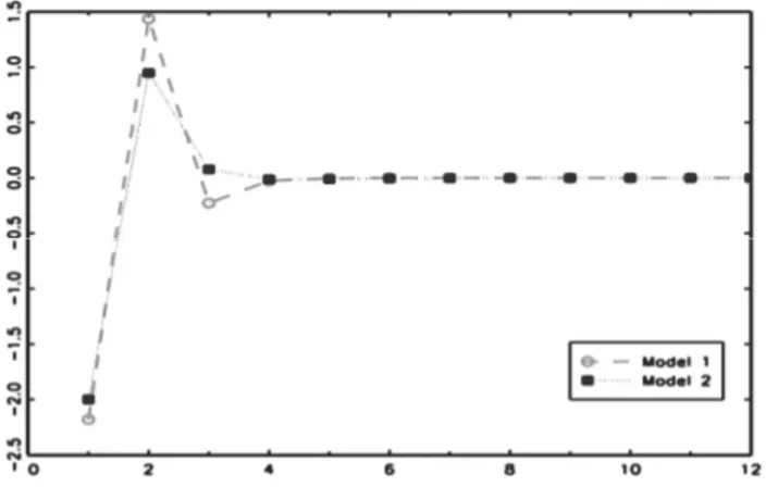
Indeed, I experienced this problem in a previous research involving the con-struction of an ARIMA model for the monthly wholesale prices index P in Italy t (Piccolo, 1972). In this circumstance, I compared two models for P : t
2 2 2 Model 1: (1 1.30 0.40 ) log( ) = (1 0.12 ) Model 2: (1 0.45 ) log( ) = (1 0.45 0.05 ) t t t t B B P B a B P B B b
by plotting the Autoregressive coefficients (j) obtained from the ARIMA operators, as
re-ported in Figure 1. In that occasion, I was comparing an ARMA(2,1) model for the inflation rate with an ARMA(1,2) model for the acceleration rate 2log( )
t
P
of
the wholesale prices. It is evident that when comparing linear models fitted to the same data set the visual inspection of the original coefficient is not conclusive. On the contrary, the Autoregressive approximation enhances the strong similarity between the estimated models.
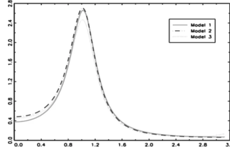
As a benchmark, we compare the following three ARMA ( , )p q models of
in-creasing complexity and characterized by the parameters: TABLE 1
ARMA (p,q) models of increasing complexity
Models 1 2 3 4 1 2 3
M1: ARMA(2,1) 0.81 -0.62 – – 0.12 – –
M2: ARMA(3,2) 1.33 -1.04 0.32 – 0.57 -0.05 – M3: ARMA(4,3) 0.48 0.09 -0.56 0.27 -0.21 0.39 -0.04
Figure 1 – Autoregressive coefficients obtained by two models for the same series.
The question is: How different are these different ARMA models? A simple way to face the problem could be via a parametric approach, by comparing the parame-ter vectors of common length:
1 1= (0.81, 0.62,0,0,0.12,0,0) ; M β 2 2= (1.33, 1.04,0.32,0,0.57, 0.05,0) ; M β 3 3= (0.48,0.09, 0.56,0.27, 0.21,0.39, 0.04) , M β
by means of a Euclidean metric defined by: (M Mi, j)= ( i j) ( i j).
β β β β (1)
This coefficient-based criterion leads to the following results:
1 2 1 3 2 3
(M M, ) = 0.868; (M M, ) = 1.123; (M M, ) = 1.911.
Thus, one reaches the wrong conclusion of a large dissimilarity among the mod-els. Instead, all the models are almost coincident since they were obtained by using the rational operators: 1 2 2 1 3 2 1 0.12 1 0.45 1 0.78 ( ) = ; ( ) = ( ) ; ( ) = ( ) 1 0.52 1 0.85 1 0.81 0.62 B B B B B B B B B B B B
Their similarity can be recognized by looking for the roots of polynomial op-erators in the complex plane, or simply by comparing their spectra as shown in Figure 2. This situation is common when we get different parametric formula-tions by means of some automatic fitting criterion.
Anyway, notice that spectra cannot be computed for non-stationary data and thus the previous visual aids fail if we need to compare ARIMA ( , , )p d q models with different orders of difference operator.
Previous evidence discourages from considering to compare parameters of ARIMA models in their rational formulation as the basis for introducing a dis-tance measure since this criterion is not resistant with respect to near-cancellation of ARMA operators.
Figure 2 – Operators in the spectral domain of three ARMA models.
The genuine idea for a metric came out as the answer to a methodological is-sue raised during the DESEC project (1982-85), a national research aimed at convincing the Italian public Institutions to adopt a shared and unique seasonal adjustment procedure.
Given the need for the implementation of a massive seasonal adjustment ex-periment with thousands of time series, I faced the following problem: “How to choose few representative series from a large data set in order to reduce time and costs of the statistical analysis?” Formally, the problem is:
“Given a collection of time series Xj t, , select a series C *
t
X such that:
*
, ,
distance(Xj t,Xt ) =min! Xj tC". (2)
Since the series to be considered were generated from different areas with dif-ferent time lengths, the investigation required the introduction of a completely general metric. These considerations were firstly diffused among a subset of Ital-ian researchers by means of the DESEC research Technical Reports series, as “A
Distance Measure for ARIMA Models” (RS 21/1984).
The journal “Statistica” published the first paper on the new proposed metric (Piccolo, 1984a) and the distribution of the maximum likelihood (ML) estimator of the metric for pure AR processes was presented at the ASA Conference in Washington (Piccolo, 1989). Then, after a long revision process, a contribution on this topic (submitted in 1986) appeared in “Journal of Time Series Analysis” (Pic-colo, 1990) and this paper became the standard international reference for the AR metric.
It is worth considering that other criteria are based on AR coefficients. In speech recognition analyses, the AR coefficients denoted as LPC (=Linear Pre-dictor Coding) were used in order to synthesize the voice signals for a specific word (Gray and Markel, 1976); however, the method was finalized only to fitting and testing purposes as in Basawa et al. (1984). In this respect, De Souza (1977) and Thomson and De Souza (1985) introduced the Mahalanobis distance be-tween AR models and derived its distributional properties. Many recent medical applications in ECGs and EEGs classifications still refer to this kind of approach (Kosĕc, 2000; Ge et al., 2002).
For many years, the AR metric has been used in several fields (with some original emphasis on seasonal adjustment procedures, as reported by Agustin Maravall, Spain and David Findley, Usa) and many statistical papers have been published. From the methodological point of view, a significant advancement on these topics has been achieved thanks to Corduas (1996, 2000a) who assessed dis-tributional properties of the AR metric in a general setting, as we will discuss in section 5.
3. STATISTICAL FOUNDATIONS
Dictionaries define distance as: “the property created by the space between two objects or points; the size of the gap between two places; the interval between two times;...”
Instead, metric is: “a system of related measures that facilitates the quantifica-tion of some particular characteristic; a funcquantifica-tion of a topological space that gives, for any two points in the space, a value equal to the distance between them,...”
Then, a preliminary remark applies: distance is a concept that may be trans-formed into an operational tool by means of some conventional measure. It is cor-rect to argue in favor or against a specific metric, since a metric is strictly deter-mined by the purpose of a research: different metrics are acceptable if different objectives
are pursued.
In fact, when objects to be compared are time series, an effective metric should satisfy the following requirements:
• it is simple to compute and provides meaningful interpretation of data; • it is dependent on the stochastic structure of the data generating process; • it is implemented for the largest class of stochastic processes generally
con-sistent with observed time series;
• it is not dependent both on the length of data and the unit of measurement of time series;
• it is robust with respect to local anomalies in the series to be compared. In addition, our approach relies on the fundamental paradigm which relates a
time series to the generating stochastic process via a statistical model. As a consequence,
we will define the metric on a well defined space of stochastic processes which is adequate to generate almost any real time series. The statistical determination of the features of such processes may be effectively recovered on the basis of the
observed realizations by means of inferential procedures, which are consistent and asymptotically efficient.
From a statistical point of view, the AR metric is justified by a fundamental theorem which we quote from Brockwell and Davis (1991, 130-133): “for any stationary process with a continuous spectrum ( )f there exists a finite order AR ( )p whose spectrum fAR( ) is as close as possible in absolute value to
( )
f uniformly on [ , ]”.
The theorem is extended to moving average (MA) processes and, for numeri-cal efficiency, to mixed ARMA structures. As a consequence, the AR operator provides the simplest and effective approximation of any stationary process or any process that may be transformed to stationarity. In fact, the theorem applies to both linear and not linear processes.
Specifically, given the process X , we consider ARIMA models for t
= ( )
t t t
Z g X , where f Z is obtained after g -transforming t X (in order to re-t duce asymmetries, improve Gaussianity and take into account of non-linearities) and after removing any deterministic components f (such as trading days, cal-t endar effects, outliers and mathematical functions of time, including constants).
Hereafter, we will refer to Box and Jenkins (1970) standard notation and we will assume that Z is a zero mean invertible ARIMA process defined as: t
( ) d D = ( ) ,
s t t
B Z B a
(3)
where a is a White Noise (WN) process with constant variance t 2<
a
. If a t
is a Gaussian process, given the initial values, the operators ( ), ( ) B B and the WN variance 2
a
characterize the probability distribution of the process Z . t The polynomials ( ) = ( ) ( ) B B Bs and ( ) = ( ) ( ) B B Bs , for any s , 0 have no common factors, and all the roots of ( ) ( ) = 0 B B lie outside the unit circle. We denote by the class of invertible linear stochastic processes
t
Z ARIMA such that the MA operators have all the roots outside the unit circle.
The invertibility assumption ensures the absolute (and squared) convergence of
the j coefficients so that Z can be represented in terms of its past values ac-t cording to: 1 1 2 2 ( ) =B Zt at Zt= Zt Zt at, (4) where: 1 =1 ( ) = (1 ) (1d s D) ( ) ( ) = 1 j j j B B B B B B
.1 1 2 2
= ,
t t t
F Z Z (5)
whereas a corresponding orthogonal representation is: Zt =Ft a Ft, t at,t. Let X t and Y t be invertible processes whose forecast functions may be expressed via the corresponding AR coefficients:
1, 2, , 1, 2, ,
= ( , , , ); = ( , , , ).
x x x j x y y y j y
π π (6)
Then, given the absolute convergence of the -sequences in , Piccolo (1984a, 1990) introduced a metric between two ARIMA processes, X and t Y , t with given orders, as the Euclidean distance between the -weights of their cor-responding AR( ) formulation:
1 2 2 , , =1 ( , )=[( ) (' )] = ( ) . t t x y x y j x j y j d X Y π π π π
(7)The most immediate and convincing interpretation of the AR metric stems from the following result: given the same set of initial values, the distance between two
ARIMA processes is zero if and only if the corresponding models produce the same forecasts.
The distance (d X Y is a well defined measure of structural dissimilarity t, )t among any processes belonging to and its value is determined by all the com-ponents of the stochastic structures to be compared. Notice that, if both X t and Y t , then (d X Y is always well defined irrespective of the fact that one t, )t or both processes are stationary or non-stationary.
Since AR metric takes rational operators into account before their expansion into j coefficients, it may be considered fairly robust with respect to over-parameterization (although we discourage this practice in time series inference).
We mention a recurrent objection against the AR metric which assesses that it does not take the WN variance into account. Indeed, this quantity is a mere scale factor depending on the measurement unit: it is well known that, for stationary linear processes, the noise-to-series variances ratio is a function of the process parameters. To face the objection, different proposals have been introduced in the literature and we just quote two of them since they are motivated by different needs.
In order to detect influential observations, Peña (1990) considered the squared Mahalanobis AR distance to assess how the parameters of a model change when each observation is in turn removed from the time series and replaced by the es-timated missing value. Such measure is not a metric; it explicitly depends on the WN variance, and it turns out that it is related to the squared Euclidean distance between the one step ahead forecast values of the series. Consequently, it is strongly affected by the scale unit.
Similar considerations apply to the proposal of Tong and Dabas (1990), which introduced similarity and dissimilarity measures for clustering the residuals obtained from various statistical models fitted to the same time series, and to Maharaj (1996, 1999, 2000) results aimed at classifying and clustering time series data.
These criteria are effective for the purposes that the Authors considered (out-liers detection, clustering of several homogeneous time series, comparing residu-als from different models fitted to the same series, and so on) but they cannot be used to compare time series obtained by completely different data generating processes. For instance, these proposals are not even useful to compare a model fitted to a time series with a model fitted to the logarithm of the same series. 4. TOPOLOGICAL PROPERTIES
The introduction of (d X Y over t, )t transforms in a metric space, and any sub-class of (e.g. the AR MA ARMA IMA, , , classes) is a well defined metric space with respect to the same metric.
Any WN process is the origin for the metric space , and for any Z t , the
norm is defined by: 2<
j
j
. In addition, we are able to define the angle between two processes X t , Y t by means of:1/2 2 2 , , , , cos( ) = j x j y j x j y . j j j
(8)The metric space is isometric with respect to seasonal processes since, for any > 0
s :
( ( ) , ( ) ) = ( ( )s , ( ) ).s
x t y t x t y t
d B X B Y d B X B Y (9)
For multivariate applications of the metric it is important to define the distance of a single series from a given class, and the diameter of a class of time series models.
Given a series X t and a class of time series models , the distance of t
X from is defined by:
( t, ) = inf { ( t, t), t }.
dist X d X Y Y (10)
For any class , the diameter is defined by:
( ) = sup{ ( t, ),t t , t }.
Finally, it may be shown that the sub-class of AR processes has a finite diame-ter. Notice that the size of the diameter has an immediate impact on the reliability of a selected time series model to represent the whole set.
It is of interest to consider a prototypical example for computing the AR met-ric. Let X t and Y t two ARMA(1,1) processes. From a formal expansion of the corresponding j coefficients:
1 1 , = ( ) j ; , = ( ) j ; =1, 2, j x x x x j y y y y j we obtain: 2 2 2 2 2 ( ) ( )( ) ( ) ( , ) = 2 . 1 1 1 y y x x y y x x t t x y x y d X Y
This result is completely general for computing also the distance between proc-esses belonging to the sub-classes AR(1), MA(1), ARIMA(0,1,0), ARIMA(0,1,1): it suffices, in the previous formula, to let some parameters equal to 0 and/or 1.
For instance, by letting x =y= 0 and x =1 x; y=1y, we obtain the distance between the ARIMA(0,1,1) processes implied by the so-called
exponen-tial smoothing procedure (EWMA processes).
By letting x=y= 1, we obtain the distance between two non-stationary MA(1) processes: 2 2( , ) = 2 ( ) . (1 )(1 )(1 ) x y x y x y d X Y
From the last expression, we get:
2 2 1 1 1 1 ( , ) = ; ( , ) = . lim lim 1 1 y x y x x y d X Y d X Y
In this case, the metric is well defined also for borderline non-invertible ARIMA processes (Piccolo, 1990). Notice that here Xt and Yt are cointegrated of order 1 and borderline non-invertible processes.
5. COMPUTATIONAL ISSUES AND STATISTICAL INFERENCE
From an operational point of view the AR metric addresses several problems related to the correct specification of time series models to be compared, efficient estimation of parameters and effective numerical computations of the AR coeffi-cients. We defer to Corduas and Piccolo (2008) for most of them and we limit
ourselves to briefly discuss the model selection step given that specification is one of the critical and controversial point with respect to a correct use of this metric.
First of all, computations are feasible if one knows processes whereas in the real world researcher need to infer on them. Thus, if one needs to compare sev-eral ARIMA processes on the basis on their finite realizations, it is effective to obtain the estimation of the parameter vector by maximum likelihood methods which require a specification of the orders of the ARIMA models. In this respect, strategies split into ad hoc modelling criteria (for small/moderate size of the data set) and automatic modeling via AIC or BIC criteria (for large data set).
As a matter of fact, one has to choose between ad hoc modelling of all series or to rely on some automatic identification criterion, within a predefined class of models. In this area, some caution is necessary since most of the published works compare the AR metric with alternative measures by means of massive automatic selection criteria. In these cases, we are not convinced that comparison is really performed among metrics and not among selection criteria.
When the number of series to be analyzed may be conveniently handled, we always prefer ad hoc modelling procedures before using AR metric since the strength of the proposal relies on the possibility to fit the ARMA operators to real data in an efficient way: this mostly applies when some doubt concerns the use of non-stationary operators.
Afterwards, the distribution of the distance estimator is required to assess sig-nificant dissimilarities. A preliminary result, concerning the comparison of AR models based on ML estimators, was obtained by Piccolo (1989). Instead, Sarno (2000, 2001) discusses asymptotic distribution of the metric derived from least squares estimators when MA processes are involved.
The asymptotic distribution of the metric for any ARIMA processes in has been fully derived by Corduas (1996), together with efficient algorithms (Corduas, 2000a). Briefly, assuming that efficient ML methods have been implemented for estimating the =k p q P Q parameters of the ARMA models to be com-pared, it can be shown that, under the null hypothesis H π0: x =π : y
2 2 =1 ˆ ( , )t t k j g j, j d X Y
(12) where 2 g j are independent Chi-square random variables, with g degrees of j freedom given by the multiplicity of each eigenvalue (usually, g ) and j 1 j are the eigenvalues of a convenient matrix C0 of order (k k ).
We write the non-stationary π coefficients as the linear transformation:
= A
π Aπ v of the stationary coefficients π , for some non-stochastic matrix A
A and vector v. For ARIMA models, the matrix C0 is defined by:
1 1
0= (nx ny ) ' ',
where n and y nx are the lengths of the realizations of Xt and Yt, respectively, and the matrices A B V, , can be derived from the model operators by effective algorithms.
For computing critical values, standard results may be applied to this problem: specifically, we may exploit results on the approximation of a linear combination of square random variables by means of a linear transformation of a Chi-square, with convenient degrees of freedom (as proposed by Corduas, 1996), or we may apply a Box-Cox transformation to the estimator ˆd in order to improve its convergence to Normality (as proposed by D’Elia, 2000). An updated account of this approach for clustering purposes has been obtained by Corduas and Pic-colo (2008).
Finally, as explorative tools for visualizing clusters and representations induced by the AR metrics, we quote dendrograms generated by a cluster analysis based on such distance, visual displays (Tran-Luu and DeClaris, 1997), multidimen-sional scaling representations (Piccolo, 1984b) and graph methods (Sarno, 2005; Palomba et al., 2008).
6. EXTENSIONS AND GENERALIZATIONS OF THE AR METRIC
Distance is an ubiquitous concept in Statistics and it is able to meet most of the need for empirical analysis. Then, the AR metric has been applied in several scientific fields such as Economics, Finance, Demography, Medicine, Linguistic, Signal processing, Environmental Sciences, Hydrology and Meteorology, Seis-mology, Astronomy, and so on.
In addition to the standard comparison of time series and statistical mod- els, the literature registers different variants of the original proposal of an AR metric:
• methodological arguments aimed at extending the proposal from a statistical point of view;
• statistical methods aimed at specific objectives;
• fields of applications and different perspectives leading to an effective usage of a metric among time series models.
6.1 Generalizations and methodological extensions
Firstly, the AR metric may be generalized in order to compare (long-memory) fractional difference processes Z t ARFIMA( , , )p d q , when | |< 0.5d . In this case, for the fractional difference operator d = (1B)d we get:
1 2 2 =1 (1 2 ) ( ) = ( 1) , = 1, 2, ; ( ) = 1< . (1 ) i i i i d d d i d i d
Remember that Z t as long as > 0.5d and the Euclidean distance be-tween two -sequences is well defined even if one or both are generated by AR-FIMA operators. In this way, the AR metric is generalized to the class of invert-ible ARFIMA processes and may be correctly applied if one or both processes encompass long-memory behaviour (Corduas and Piccolo, 2006). Instead, most of the alternative proposals of the literature cannot share this remarkable prop-erty with the AR metric.
A second relevant extension of the AR metric has been proposed by Otranto (2004, 2008) for the classification of the volatility of financial time series gener-ated by GARCH models and further developed in several directions, even multi-variate (Otranto, 2009, 2010; Lisi and Otranto, 2010; Otranto and Trudda, 2008a, 2008b). The starting point is to apply the AR metric to measure the distance be-tween squared noise processes; then, cluster algorithms are applied in order to classify the volatility of several stock prices and to study their interdependence. The joint application of the AR metric to both ARIMA and GARCH model components proves to be a sound extension of the approach since it accounts for important components often detected in the majority of real time series when we are faced with clustering and discrimination objectives in economic and financial data sets.
In the econometric arena, a significant contribution to enlarge the spectrum of applications derives from the idea that the AR metric helps in detecting the rela-tionship between feedback in stochastic systems and thus it may be an useful tool for testing Granger causality (Triacca, 2004a). This approach has been recently generalized in a multivariate context by Di Iorio and Triacca (2011) who formally proved that for checking non-causality in the sense of Granger is sufficient to compute the AR metric among two univariate processes. Some simulation ex-periments and a real case study sharply favour their proposal with respect to standard econometric tests thanks to a dominant power function.
6.2 Further statistical developments
Corduas (2000b) exploited the AR metric as an estimation method in order to find the fractional value of d such that the process d =
t zt
Z a
is as close as pos-sible to the X t ARMA(1,1) process defined by: (1B X) t= (1B a) xt, where the closeness is measured by the AR metric.
Then, given the estimates βˆ =( , ) ˆ ˆ, the problem is to find d such that: 2 ° 2 1 =1 =1 ˆ ˆ ˆ ˆ ( ) = [ ( ) ( )] L ( 1)i ( )( )i = min! i i i i d G d d i
β
(14)for some fixed =100,150L , say. Further aspects of the approach have been de-veloped by Corduas and Piccolo (2001, 2003, 2006); D’Elia and Piccolo (2002a, 2002b).
A different proposal aimed at a spectral decomposition of the AR metric has been introduced by Iannario and Piccolo (2011) and their result relies on a theo-rem proved for computing this distance in an effective way. In fact, Corduas (1992a) showed that: the squared AR metric is always the variance of a well defined
station-ary process. Specifically, we denote by , , =| |, = 1, 2, . j j x j y j
the absolute difference of the AR expansion of processes X t and Y t . Then, we introduce the stationary process:
1 1 2 2 = = ( ) , t t t t t W B where 2 1 (0, ) t WN
and the coefficients j are obtained as:
1 1 = j , = 1, 2, j j It is immediate to show that:
2 2 , , =1 ( t) = | j x j y| = ( , ). j Var W
d X Y (15)The process Wt is obtained by filtering the WN process t by means of a linear operator ( )B where the differences of the AR expansions of both proc-esses Xt and Yt are taken into account. It is evident that the time dynamics of
t
W reflects characteristics of both processes to be compared. Two processes Xt and Yt with similar behaviour produce small j coefficients while processes with quite dissimilar structures induce large coefficients j.
Although Wt is a fictitious process, its statistical analysis helps in investigating the structural dissimilarity among Xt and Yt as synthesized by the AR metric. The process Wt may be non-invertible but it is always stationary. Thus, it admits a symmetric spectral function defined by:
2 2 1 ( ) = | ( )| , 0 < < . g e
Then, the spectral decomposition of the AR metric immediately follows:
2
0
( , ) = ( t) = ( ) .
This result allows to ascertain whether some components at low, high, peri-odic, seasonal frequencies contribute to the determination of the value of
2( , )
d X Y . In addition, since g( )/ ( , ) d X Y2 shares all the properties of a well
defined density function over (0, ) , one should consider that a high accumula-tion of variance of Wt around some range of angular frequencies means that such components are important for explaining the computed distance among processes, and thus for increasing dissimilarities among them.
Finally, we remember that – for computing the AR metric as a variance – Cor-duas (1992b) suggested efficient numerical algorithms based on a state-space rep-resentation of the ARMA processes (Anderson and Moore, 1979) or on the auto-covariance generating function of the Wt process (Tunnicliffe Wilson, 1979).
Further methodological issues concerning the AR metric include the computa-tion of power funccomputa-tions in time series analysis (Gonzalo and Lee, 1996); the con-sequences on the metric when the series are correlated (Corduas, 1992b); a test of parallelism between two ARIMA processes (Triacca, 2004b).
6.3 Different applications and perspectives
We limit ourselves to mention the applications we are aware of in several sci-entific fields and with non standard objectives:
• regional classification of streamflow time series (Corduas, 2011);
• redundancy in environmental monitoring networks (Costanzo and Sarno, 2000; Sarno, 2005);
• data mining problems (Agrawal et al., 1994; Ng and Huang, 1999);
• validation of seasonal adjustment procedures (Corduas and Piccolo, 1999a, 1999b); selecting between direct and indirect model-based seasonal adjust-ment (Otranto and Triacca, 2002).
• representativeness of an aggregated index (Caceres et al., 1993);
• convergence of inflation rates in the EU countries (Sarno and Zazzaro, 2002; Palomba et al., 2008);
• plotting time series as objects in a multidimensional scaling space (Corduas, 1984; Piccolo, 1984b, 1987);
• comparison of stochastic components of a time series (Corduas and Piccolo, 1995); similarity among original series and canonical components (Quilis, 2004);
• time series clustering (Piccolo, 1984; Corduas, 1985b; Cano et al., 1992; Cor-duas and Piccolo, 1996; Maharaj, 1996, 2000; Grimaldi, 2004; Liao, 2005) and time series discrimination (Corduas, 2004);
• classification of multivariate time series (Maharaj, 1999; Galeano and Peña, 2000);
• detecting extreme (anomalous) behaviors in a homogeneous time series data set (Corduas and Piccolo, 1999a);
7. DISCUSSION OF RELATED ALTERNATIVES
An accurate discussion of relative merits and pitfalls of the alternatives to the AR metric is out of the objectives of this paper. We defer to the literature for an extensive treatment of such topics and briefly review some of them since they are more related with AR metric.
We mention some metrics based on autocorrelation sequences (as those proposed by Bohte et al., 1980, and Mélard and Roy, 1984) which are conceptu- ally related to well known tests in residual time series analysis, as Box and Pierce (1970) and Ljung and Box (1978) tests, for instance. In this regard, we no-tice that metrics based on the comparisons of partial autocorrelation sequences are more effective in the subspace of stationary processes (given some orthogo-nality property of their estimators), as experienced in the Monti (1994) test, for instance.
A large number of proposals aimed at clustering and/or discriminating time se-ries are based on spectral functions as those of Alagón (1989), Dargahi-Noubary and Laycock (1981), Kakizawa et al. (1998), Kazakos and Papantoni-Kazakos (1980), Shumway (1982, 2003) and Shumway and Unger (1974) and noticeable those derived by comparing periodograms and log-periodograms, as Caiado et al. (2006, 2009).
Further measures are derived from divergence concepts (Corduas, 1985a; Chaudury et al., 1991; Gersh et al., 1979; Kailath, 1967), wavelet analysis (Struzik and Siebes, 1999) and forecast densities (Alonso et al., 2006).
We linger over a few proposals related to the AR metric and generated by the definition of cepstrum introduced by Bogert at al. (1962). The cepstrum coefficients
j
c are obtained by the parametric expansion of the logarithm of the spectrum
( ) Z
f of a stationary process Zt, so that: 1 = log[ ( )] , = 1, 2, 2 j j c f e d j
and 2 0= log( /(2 ))c by Kolmogorov identity. Gray and Markel (1976) pro-posed the Euclidean distance (X Yt, t) among the cepstral coefficients of two stationary processes Xt and Yt as an effective metric among time series data. The proposed metric correctly excludes the c0 coefficient arguing that it is a scale
factor. It has been applied with some interesting results by Kang et al. (1995), Kalpakis et al. (2001), Savvides et al. (2008); see also: Childers et al. (1975), Boets et
al. (2005). A weighted version of (X Yt, t) has been reformulated by Martin
(2000) who completely ignores the existence of any other metric. Recently, Maha-raj and D’Urso (2011) argument in favour of fuzzy methods involving cepstral coefficients as a basic metric for their proposal of time series clustering.
Indeed, cepstral coefficients have several properties, including relationships with spectral exponential models of Bloomfield (1973) and with the partial
auto-correlation function (Li, 2004). It is worth to observe that, with obvious nota-tions, the following identity holds:
2
2 2 2
2 =
|log[ ( )] log[ ( )]| = ( ) = 2 ( , ) log ax .
X Y xj yj t t j ay f f c c X Y
As a consequence, if the processes have different degree of non-stationarity the cepstral metric is not defined. A further problem is generated by the fact that, after few lags, the cepstral coefficients are nearly zero. This circumstance may support their computational convenience but shows that any cepstral metric is heavily determined by few AR parameters.
Finally, it is important to quote the pioneering work of Zani (1983) and the re-sults of some Italian researchers whose contributions are relevant in this area and are consistent with our perspective. Specifically, Baragona (2001) and Baragona et
al. (2001) introduced genetic algorithms to measure diversity in time series data.
Moreover, Ingrassia et al. (2003) applied functional analysis and Cerioli et al. (2004) performed clustering by means of symbolic analysis.
8. CONCLUDING REMARKS
Time and/or spectral properties are the stylized features of any time series generated by ARIMA models: these characteristics are fully conveyed by the fore-cast function. Economists use exactly the same logic leading to AR metric when they introduce the concepts of parallelism between time series, as shown by Triacca (2004b) or pairwise and multiple similarity of dynamics of phenomena introduced by Bernard and Durlauf (1996), as discussed by Palomba et al. (2008).
Thus, the AR formulation is a fundamental issue for econometric and time se-ries analysis, both for stationary and stationary processes. Notice that non-linearity and deterministic trends are excluded from our approach; thus, when these dynamics are relevant, we suggest to move towards non-parametric metrics, as for instance those discussed by Zhang and Taniguchi (1995).
A further issue to be analyzed concerns the peculiar specificity of the AR met-ric to discriminate among dynamic stmet-rictures and not among observed data, as emphasized by Cubadda (2007, personal communication). If two processes Xt and Yt are defined by different ARMA operators applied to the same WN at their time realizations are obviously deterministically related (a perfect forecast of
t
Y is possible from the knowledge of Xt) but their AR distance is positive. On the contrary, we may obtain a null AR distance between processes with the same ARMA operators even if different WN processes may generate quite different re-alizations and dynamic patterns.
Since any distance measure both enhances and hides several aspects of the compared objects, it is important to recognize that the AR metric is a distance among rational operators irrespective of time series realizations. Then, the AR
metric is a useful tool for several statistical objectives if the whole structural diversity
is the main point of the analysis. On the other hand, a spectral metric could be more effective if the comparison involves local features (e.g. long memory, periodic pat-terns, seasonality, etc.).
As a matter of fact, in the AR metric, the contribution of each j coefficient to the stochastic components of the process is spread over all the angular fquencies; thus, this metric should not be applied if our concept of closeness is re-lated to some specific frequential component. For instance, Caiado et al. (2006) proved by simulation that a periodogram-based measure may result more effec-tive than the AR metric for detecting a non-stationary behaviour. Similarly, Pic-colo and Corduas (2006) supported a spectral metric when the angular frequen-cies around origin are the central issue for assessing the similarity among station-ary and fractional difference processes.
As a conclusion, we emphasize that the AR metric is well defined for station-ary and non stationstation-ary, short and long memory, seasonal and non seasonal sto-chastic processes; it encompasses the relevant time and frequential domain fea-tures of a time series dynamics in a parsimonious parametric way. Thus, accord-ing to our opinion and experiences, the AR metric is a powerful and wide appli-cable tool to study and understand the relationships among time series, but it also helps to produce new ideas, genuine proposals and innovative developments.
Dipartimento di Teorie e Metodi delle Scienze DOMENICO PICCOLO
Umane e Sociali, sezione di Scienze Statistiche Università degli Studi di Napoli Federico II
REFERENCES
R. AGRAWAL, C. FALOUTSOS, A. SWAMI,(1994),Efficient similarity search in sequence databases, 4th
Proceedings of F.O.D.O.93 in Lecture Notes in Computer Science, Springer Verlag, New York: 69-84.
J. ALAGÓN, (1989), Spectral discrimination of two groups of time series, Journal of Time Series
Analysis, 10:202-214.
A.M. ALONSO, J.R. BERRENDERO, A. HERNÁNDEZ, B. JUSTEL,(2006), Time series clustering based on
forecast densities, Computational Statistics & Data Analysis, 51:762-776.
B.D.O. ANDERSON, J.B. MOORE,(1979),Optimal filtering. Prentice Hall, Englewood Cliffs. R. BARAGONA,(2001),A simulation study on clustering time series with metaheuristic methods, Qua-
derni di Statistica, 3:1-26.
R. BARAGONA, F. BATTAGLIA, D. CUCINA,(2001),Clustering of time series with genetic algorithms,
Met-ron, 59:113-130.
I.V. BASAWA, L. BILLARD, R. SRNIVASAN,(1984), Large sample tests of homogeneity for time series,
Bio-metrika, 71:203-206.
A.B. BERNARD, S.N. DURLAUF,(1996), Interpreting tests of the convergence hypothesis, Journal of
Eco-nomics, 71:1161-173.
P. BLOOMFIELD, (1973), An exponential model for specrtum of a scalar time series, Biometrika,
60:217-226.
J. BOETS, K. AND DE COCK, M. AND ESPINOZA, B. DE MORR,(2005), Clustering time series, subspace
J. BOETS, K. DE COCK, M. ESPINOZA, B. DE MORR, (2008), Clustering of biological time series by cepstral
coefficients based distances, Communications in Informations and Systems, 41:2398-2412.
B.P. BOGERT, M.J. HEALY, J.W. TUKEY,(1962), The quefrency analysis of time series for echoes: cepstrum,
pseudo-autocovariance, cross-ceptstrum and saphe cracking. In M. ROSENBLATT (eds.), Proceedings
of the Symposium on Time Series Analysis, J. Wiley & Sons, New York: 209-263.
Z. BOHTE, D. CEPAR, K. KOSMELIJ,(1980), Clustering of time series, Proceeding of 1980
Computa-tional Statistics Meeting in COMPSTAT80: 587-593.
G.E.P. BOX, G.M. JENKINS,(1970), Time series analysis: forecasting and control (revised edition, 1976).
Holden-Day, San Francisco.
G.E.P. BOX, D.A. PIERCE,(1970), Distribution of the residual autocorrelations in autoregressive integrated
moving average time series models, Journal of the American Statistical Association,
65:1509-1526.
P.J. BROCKWELL, R.A. DAVIES, (1991), Time series: theory and methods (2nd edition).
Springer-Verlag, New York.
J.J. CACERES, V.J. CANO, F.J. MARTIN, (1993), Analysis de la representatividad del I.P.I. agregado.
Documento de trabajon n.45, Universidad de la Laguna, Tenerife.
J. CAIADO, N. CRATO, D. PEÑA,(2006), A periodogram-based metric for time series classification,
Com-putational Statistics & Data Analysis, 50:2668-2684.
J. CAIADO, N. CRATO, D. PEÑA,(2009), Comparison of time series with unequal length in the frequency
domain, Communications in Statistics-Simulation and Computation, 38:527-540.
V.J. CANO, F.J. MARTIN, J.J. CACERES,(1992), Medida de distancia entre modelos ARIMA. Una
aplica-cion a los Indices de Precios Percibidos por los Agricultores, Investigaaplica-cion Agraria, 7:33-45.
A. CERIOLI, S. INGRASSIA, A. CORBELLINI, (2004), Classificazione simbolica di dati funzionali:
un’applicazione al monitoraggio ambientale. In C.N. LAURO, C. DAVINO (eds.), Data
min-ing e analisi simbolica, F. Angeli, Milano.
G. CHAUDURY, J.D. BORWARKAR, P.R.K. RAO,(1991), Bhattacharyya distance based linear discriminant
function for stationary time series, Communications in Statistics. Theory and Methods,
20:2195-2205.
D.G. CHILDERS, D.P. SKINNER, R.C. KEMERAIT,(1975),The cepstrum: a guide to processing,
Proceed-ings of the IEEE, 65:1428-1443.
M. CORDUAS, (1984), Un programma per la rappresentazione dei modelli ARIMA, Rivista di Stati-
stica Applicata, 17:211-214.
M. CORDUAS,(1985a),Alcune considerazioni statistiche sulla divergenza tra processi lineari, Statistica,
XLV:393-401.
M. CORDUAS, (1985b), Una classificazione statistica delle serie economiche italiane mediante modelli
ARIMA, Note Economiche, 6:163-178.
M. CORDUAS, (1992a), Misure di distanza tra serie storiche e modelli parametrici, Quaderni del-
l’Istituto Economico Finanziario, n.3. Università di Napoli Federico II.
M. CORDUAS, (1992b), Una nota sulla distanza tra modelli ARIMA per serie storiche correlate, Stati-
stica, LII:512-520.
M. CORDUAS,(1996), Uno studio sulla distribuzione asintotica della metrica Autoregressiva, Statistica,
LVI:321-332.
M. CORDUAS, (2000a), La metrica Autoregressiva tra modelli ARIMA: una procedura in linguaggio
GAUSS, Quaderni di Statistica, 2:1-37.
M. CORDUAS, (2000b), Preliminary estimation of ARFIMA models, in J.G. BETLEHEM, P.G.M. VAN DER HEIJDEN(eds.), Proceedings in Computational Statistics, Physica Verlag, Heidelberg,
247-252.
M. CORDUAS,(2003), Il confronto tra serie storiche nell’analisi statistica di dati dinamici, “Atti della
M. CORDUAS, (2004), Time series discrimination using AR metric, Proceedings of XLII Riunione
Scientifica SIS, CLEUP, Padova, 143-146.
M. CORDUAS, (2007), Comparing time series: shape-based or structural similarities?, Proceedings of
CLADAG-2007 Meeting, EUM,University of Macerata, 69-72.
M. CORDUAS,(2011), Clustering streamflow time series for regional classification, Journal of
Hydrol-ogy, forthcoming.
M. CORDUAS, D. PICCOLO, (1995), Mutamenti strutturali della natalità e differenziazioni regionali,
“Atti del Convegno SIS: “Continuità e discontinuità nei fenomeni demografici”, Uni-versità degli Studi della Calabria, Editore Rubettino, 315-322.
M. CORDUAS, D. PICCOLO, (1996), Time series clustering of the Italian Consumer Price Indices: a model
approach, Quaderni di Ricerca ISTAT, Istituto Nazionale di Statistica, Roma.
M. CORDUAS, D. PICCOLO,(1999a), An application of the AR metric to seasonal adjustment, Bulletin
of the International Statistical Institute, International Statistical Institute, 217-218.
M. CORDUAS, D. PICCOLO, (1999b),On the use of AR metric for seasonal adjustment, Proceedings of
the International Conference CLADAG-99, University of Rome “La Sapienza”, 1-4.
M. CORDUAS, D. PICCOLO,(2001), Fractional differencing models estimations: some new approaches, in D. PICCOLO, L. UBERTINI(eds.), Metodi Statistici e Matematici per l’Analisi delle Serie Idrologiche,
CNR-GNDCI n.2136, Roma, 73-79.
M. CORDUAS, D. PICCOLO, (2003), Determinazione del lag ottimale nelle stime di minima distanza del
parametro alle differenze frazionarie, in D. PICCOLO, L. UBERTINI(eds.), Metodi Statistici e
Mate-matici per l’Analisi delle Serie Idrologiche, CNR-GNDCI n.2818, Roma, 73-80.
M. CORDUAS, D. PICCOLO, (2006), Short and long memory unobserved components in hydrologic time
series, Physics and Chemistry of the Earth, 31:1099-1106.
M. ORDUAS, D. PICCOLO, (2008), Time series clustering and classification by the autoregressive metric,
Computational Statistics & Data Analysis, 52:1860-1872.
G.D. COSTANZO, E. SARNO,(2000), La metrica autoregressiva per la valutazione e ottimizzazione di
sistemi di monitoraggio ambientale, Quaderni di Statistica, 2:205-220.
A. D’ELIA,(2000), Uno studio sull’asimmetria dello stimatore della metrica Autoregressiva, Quaderni
di Statistica, 2:59-84.
A. D’ELIA, D. PICCOLO,(2002), A comparison among several methods for estimating the fractional
differ-encing parameter, in S. KINKE, P. AHREND, L. RICHTER(eds.), Proceedings of the Compstat 2002
Conference, Humboldt-Universitat, Physica Verlag, Berlin, 1-2.
A. D’ELIA, D. PICCOLO,(2002), Stimatori di minima distanza del parametro alle differenze frazionarie,
Quaderni di Statistica, 4:115-138.
G.R. DARGAHI-NOUBARY, P.J. LAYCOCK,(1981), Spectral ratio discriminants and information theory,
Journal of Time Series Analysis, 2:71-86.
P.V. DE SOUZA,(1977), Statistical tests and distance measures for LPC coefficients, “IEEE
Transac-tions on Acoustics, Speech, and Signal processing”, ASSP-25(6):554-559.
F. DI IORIO, U. TRIACCA,(2011), Testing for Non-causality by using the Autoregressive Metric.
Tech-nical report, Department TEOMESUS, University of Naples Federico II, submitted.
P. GALEANO, D. PEÑA,(2000), Multivariate analysis in vector time series, Resenhas, 4:383-404.
D. GE, N. SRINIVASAN, S.M. KRISHNAN,(2002), Cardiac arrhythmia classification using autoregressive
modeling, Biomedical Engineering OnLine, www.biomedical-engineering-online.com.
W. GERSH, F. MARTINELLI, J. YONEMOTO, M.D. LOW, J.A.MCEWAN, (1979), Automatic classification of
electroencephalograms: Kullback-Liebler nearest neighbor rules, Science, 205:193-195.
J. GONZALO, T.H. LEE, (1996), Relative power of t type tests for stationary and unit root processes,
Journal of Time Series Analysis, 17:37-47.
A.H. GRAY, J.D. AND MARKEL, (1976), Distance measures for speech processing, “IEEE Transactions
S. GRIMALDI,(2004), Linear parametric models applied on daily hydrological series, Journal of
Hy-drological Engineering, 9:383-391.
M. IANNARIO, D. AND PICCOLO,(2011), Spectral decomposition of the AR metric, “Proceedings of
the SIS Conference”, in press, SIS-2010, Springer-Verlag, Berlin.
S. INGRASSIA, A. CERIOLI, A. CORBELLINI, (2003), Some issues on clustering of functional data, in M. SCHADER, W. GAUL, M. VICHI (eds.), Between Data Science and Applied Data Analysis, Springer,
Berlin, 49-56.
T. KAILATH,(1967), The divergence and Bhattacharyya distance measures in signal selection, “IEEE
Transactions on Communications in Technology”, 15:52-60.
Y. KAKIZAWA, R.H. SHUMWAY, M. TANIGUCHI,(1998), Discrimination and clustering for multivariate
time series, Jounral of the American Statistical Association, 93:328-340.
K. KALPAKIS, D. GADA, V. PUTTAGUNTA, (2001),Distance measures for effective clustering of ARIMA
time series, “Proceedings of the IEEE International Conference on Data Mining”,
ICDM’01, San Jose, California, 273-280.
W. KANG, C. CHENG, J. LAI, H. TSAO,(1995), The application of cepstral coefficients and maximum
like-lihood method in EGM pattern recognition, “IEEE Transactions on Biomedical
Engineer-ing”, 42:777-785.
D. KAZAKOS, P. PAPANTONI-KAZAKOS,(1980), Spectral distances between Gaussian processes, “IEEE
Transactions on Automatic Control”, 25:950-959.
D. KOSĔC,(2000), Parametric estimation of continuous non stationary spectrum and its dynamics in
sur-face EMG studies, International Journal of Medical Informatics, 58/59:59-69.
Z.J. KOVAČIĆ, (1996), Classification of time series with application to the leading indicator selection,
“Proceedings of the fifth Conference of IFCS”, number 2, 204-207.
L.M. LI,(2004), Some notes on mutual information between past and future, Journal of Time Series
Analysis, 27:309-322.
T.W. LIAO, (2005), Clustering time series data - a survey, Pattern Recognition, 38:1857-1874. F. LISI, E. OTRANTO,(2010), Clustering Mutual Funds by Return and Risk Levels, in M. CORAZZA,
C. PIZZI (eds.), Mathematical and Statistical Methods for Actuarial Sciences and Finance,
MAF2010, Springer-Verlag, Berlin, 183-191.
G.M. LJUNG, G.E.P. BOX, (1978), On a measure of lack of fit in time series models, Biometrika,
65:297-303.
E.A. MAHARAJ, (1996), A significance test for classifying ARMA models, Journal of Statistical
Computation and Simulation, 54:305-331.
E.A. MAHARAJ,(2000), Clusters of Time Series, Journal of Classification, 17:297-314.
E.A. MAHARAJ,(1999), Comparison and classification of stationary multivariate time series, Pattern
Recognition, 32:1129-1138.
E.A. MAHARAJ, P. D’URSO, (2011), Fuzzy clustering of time series in the frequency domain,
Informa-tion Sciences, 181:1187-1211.
R.J. MARTIN,(2000), A metric for ARMA processes, “IEEE Transactions on Signal
Process-ing”, 48:1164-1170.
A.C. MONTI,(1994), A proposal for residual autocorrelation test in linear models, Biometrika, 81:776-780. G. MÉLARD, R. ROY,(1984), Sur un test d’égalité des autocovariances de deux series chronologiques,
Ca-nadian Journal of Statistics, 12:333-342.
M.K. NG, Z. HUANG,(1999), Data mining massive time series astronomical data: challenges, problems
and solutions, Information and Software Technology, 41:545-556.
E. OTRANTO,(2004), Classifying the markets volatility with ARMA distance measures, Quaderni di
Statistica, 6:1-19.
E. OTRANTO, (2008), Clustering Heteroskedastic Time Series by Model-Based Procedures,
E. OTRANTO, (2009), Improving the Forecasting of Dynamic Conditional Correlation: a Volatility
De-pendent Approach. Working Paper 2009/17, submitted; under review, CRENoS.
E. OTRANTO,(2010), Identifying Financial Time Series with Similar Dynamic Conditional Correlation,
Computational Statistics & Data Analysis, 54:1-15.
E. OTRANTO, U. TRIACCA, (2002), Measures to evaluate the discrepancy between direct and indirect
model-based seasonal adjustment, Journal of Official Statistics, 18:511-530.
E. OTRANTO, A. TRUDDA,(2008a), Classifying the Italian pension funds via GARCH distance, in C. PERNA, M. SIBILLO (eds.), Mathematical and Statistical Methods for Insurance and Finance,
MAF2008, Springer-Verlag, Berlin, 189-197.
E. OTRANTO, A. TRUDDA,(2008b), Evaluating the risk of pension funds by statistical procedures, in G.M. LAKATOS (eds.), Transition Economies: 21st Century Issues and Challenges, Chapter 7,
Nova Science Publisher, Hauppauge, NY, 189-204.
G. PALOMBA, E. SARNO, A. ZAZZARO,(2008), Testing similarities of short-run inflation dynamics among
EU-25 countries after the Euro, Empirical Economics, 37:231-270.
D. PEÑA,(1990), Influential observation in time series, Journal of Business and Economic
Statis-tics, 8:235-242.
D. PICCOLO, (1972), D. Analisi statistica dei prezzi all’ingrosso in Italia:1956-71, Rassegna
Economica, XXXVI:1555-1599.
D. PICCOLO,(1984a), Una topologia per la classe dei processi ARIMA, Statistica, XLIV:47-59, a. D. PICCOLO, (1984b), Una rappresentazione multidimensionale per modelli statistici dinamici, “Atti
della XXXII Riunione Scientifica della SIS”, pp. 149-160, b.
D. PICCOLO, (1987), Problemi di confronto in rappresentazioni alternative di fenomeni dinamici, Qua-
derni di Statistica e Econometria, IX:1-10.
D. PICCOLO, (1989), On a measure of dissimilarity between ARIMA models, “Proceedings of the
A.S.A. Meetings, Business and Economic Statistics Section”, pp. 231-236, ASA, Wash-ington D.C.
D. PICCOLO, (1990), A distance measure for classifying ARIMA models, Journal of Time Series
Analysis, 11:153-164.
D. PICCOLO, (2007), Statistical issues on the AR metric in time series analysis, “Proceedings of the
2007 Intermediate Conference”, pp. 221-232, SIS-2007, CLEUP, Padova.
D. PICCOLO, M. CORDUAS, (2006), Spectral approximation to the fractional differencing operator, in D. PICCOLO, L. UBERTINI (eds.), Metodi Statistici e Matematici per l’Analisi delle Serie Idrologiche,
CNR-GNDCI n.2908, Roma, 11-23.
E.M. QUILIS,(1990), Una aplicación de los modelos BVAR estacionales, Economía, Instituto
Na-cional de Estadistíca, Madrid, 4:207-214.
E. SARNO, (2000), The behaviour of the AR metric for MA models comparisons, in SIS(eds.),
“Proceedings of the XL Scientific Conference”, University of Florence, Firenze, 149-152.
E. SARNO,(2001), Further results on the asymptotic distribution of the Euclidean distance between MA
models, Quaderni di Statistica, 3:165-175.
E. SARNO,(2005), Testing information redundancy in environmental monitoring networks,
Environ-metrics, 16:71-79.
E. SARNO, A. ZAZZARO,(2002), An index of dissimilarity among time series: an application to the
infla-tion rates of the EU countries, in S. KLINKE, P. AHREND, L. RICHTER (eds.), Proceedings of
COMP-STAT 2002, Springer, Berlin, 1-2.
R.H. SHUMWAY, (1982), Discriminant analysis for time series, in P.R. KRISHNAIAH, L.N. KANAL (eds.),
Handbook of Statistics, vol. 2., North Holland, Amsterdam, 1-46.
R.H. SHUMWAY,(2003), Time-frequency clustering and discriminant analysis, Statistics and
R.H. SHUMWAY, A.N. UNGER,(1974), Linear discriminant functions for stationary time series, Journal
of the American Statistical Association, 65:1527-1546.
Z.R. STRUZIK, A. SIEBES,(1999), The Haar wavelet in the time series similarity paradigm,
“Proceed-ings of the Third European Conference on Principles of Data Mining and Knowledge Discovery”, Springer, Prague, 12-22.
P.J. THOMSON, P. DE SOUZA, (1985), Speech recognition using LPC distance measures, in E.J. HANNAN, P.R. KRISHNAIAH, M.M. RAO (eds.), Handbook of Statistics, North Holland, Amsterdam,
389-412.
H. TONG, P. DABAS,(1990), Cluster of time series, Journal of Applied Statistics, 17:187-198. T.D. TRAN-LUU, N. DECLARIS, (1997), Visual heuristics for data clustering, “IEEE Transactions on
Systems”, Man and Cybernetics, 1:19-24.
U. TRIACCA,(2004a), Feedback, causality and distance between ARMA models, Mathematics and
Computers in Simulation, 64:679-685.
U. TRIACCA,(2004b), A note on distance and parallelism between two ARIMA processes, Quaderni
di Statistica, 6:21-29.
G. TUNNICLIFFE WILSON,(1979), Some efficient computational procedure for high order ARMA
mod-els, Journal of Statistical Computation and Simulation, 8:301-309.
S. ZANI,(1983), Osservazioni sulle serie storiche multiple e l’analisi dei gruppi, inD. PICCOLO(eds.),
Analisi moderna delle serie storiche, Convegno nazionale 1981, F. Angeli, Milano, 263-274.
G. ZHANG, M. TANIGUCHI,(1995), Nonparametric approach for discriminant analysis in time series,
Nonparametric Statistics, 5:91-101.
SUMMARY
The Autoregressive metric for comparing time series models
The Autoregressive metric was firstly introduced in 1983 as a tool for choosing a rep-resentative element from a large collection of time series and for clustering temporal data. The proposal has been extended to many contexts and has raised increasing interests in both time series methods and applications. The main results concerning this metric, its asymptotic distribution and some operational and comparative issues are presented. A discussion about the merits of this distance criterion and some caveats about its usage conclude the paper.