Development of Data-Driven Dispatching Heuristics for Heterogeneous HPC Systems

(1)

Alma Mater Studiorum · Università di

Bologna

SCUOLA DI SCIENZE

Corso di Laurea Magistrale in Informatica

DEVELOPMENT OF DATA-DRIVEN

DISPATCHING HEURISTICS FOR

HETEROGENEOUS HPC SYSTEMS

Relatore:

Chiar.mo Prof.

Ozalp Babaoglu

Correlatore:

Chiar.ma Prof.ssa

Zeynep Kiziltan

Presentata da:

Alessio Netti

II Sessione

Anno Accademico 2016/2017

(2)

(3)

“When we first went out into space, you showed me the Galaxy. Do you remember?” “Of course.” “You speeded time and the Galaxy rotated visibly. And I said, as though anticipating this very time, ‘The Galaxy looks like a living thing, crawling through space.’ Do you think that, in a way, it is alive already?” [Isaac Asimov - Foundation’s Edge]

(4)

(5)

Introduzione

Nell’ambito dei sistemi High-Performance Computing, realizzare euristiche di

dispatching efficaci è fondamentale al fine di ottenere buoni livelli di Quality

of Service. Per dispatching intendiamo i metodi tramite cui i task (o jobs)

sottomessi dagli utenti al sistema sono selezionati e preparati per l’avvio su di esso, sia in termini temporali che di allocazione delle risorse. In questo contesto, ci concentreremo sul design e l’analisi di euristiche di allocazione per il dispatching; tali euristiche saranno progettate per sistemi HPC

etero-genei, nei quali i vari nodi possono essere equipaggiati con diverse tipologie di

unità di elaborazione. Alcune di esse, inoltre, saranno di tipo data-driven, e dunque sfrutteranno l’informazione fornita dal workload corrente in modo da stimare parametri ignoti del sistema, e migliorare la propria efficacia. Considereremo in particolare Eurora, un sistema HPC eterogeneo realizzato da CINECA, a Bologna, oltre che un workload catturato dal relativo log di sistema, contenente jobs reali inviati dagli utenti. Un contesto di tal genere, in piccola scala ed eterogeneo, costituisce l’ambiente perfetto per la valu-tazione di diversi metodi di dispatching. Tutto ciò è stato possibile grazie ad

AccaSim, un simulatore di sistemi HPC da noi sviluppato nel Dipartimento

di Informatica - Scienza e Ingegneria (DISI) dell’Università di Bologna: Ac-caSim è uno strumento innovativo per l’analisi dei sistemi HPC, il quale ha attualmente pochissimi rivali in termini di flessibilità ed efficienza.

In particolare, quest’elaborato affronta il tema della valutazione di metodi di dispatching HPC in un ambiente simulato, insieme all’impiego di euristiche data-driven per la predizione della durata dei jobs. Ciò è stato fatto al fine di stimare l’impatto di tali tecniche sul throughput del sistema, in termini di tempi di attesa e dimensione della coda dei jobs, ancora una volta nell’ambito dei sistemi HPC eterogenei, più difficili da gestire rispetto alle controparti omogenee.

Il contributo principale di questo lavoro consiste nel design e nello sviluppo di nuove euristiche di allocazione: queste sono state impiegate insieme a metodi

(6)

di scheduling già disponibili, i quali sono stati a loro volta adattati e miglio-rati. Le euristiche sviluppate sono state poi testate con il workload di Eurora disponibile, in diverse condizioni operative, e successivamente analizzate. In-fine, si è contribuito in modo significativo allo sviluppo di diverse parti core del simulatore AccaSim.

Quest’elaborato mostra che l’impatto di diverse euristiche di allocazione sul throughput di un sistema HPC eterogeneo non è trascurabile, con variazioni in grado di raggiungere picchi di un ordine di grandezza. Tali differenze in termini di throughput sono inoltre molto più pronunciate se si considerano brevi intervalli temporali, come ad esempio dell’ordine dei mesi, suggerendoci che il comportamento a lungo termine del sistema è dettato principalmente dal metodo di scheduling utilizzato. Abbiamo inoltre osservato che l’impiego di euristiche per la predizione della durata dei jobs è di grande beneficio al throughput su tutte le euristiche di allocazione, e specialmente su quelle che integrano in maniera più profonda tali elementi data-driven. Infine, l’analisi effettuata ha permesso di caratterizzare integralmente il sistema Eurora ed il relativo workload, permettendoci di comprendere al meglio gli effetti su di esso dei diversi metodi di dispatching, nonché di estendere le nostre consid-erazioni anche ad altre classi di sistemi.

La tesi è strutturata come segue: nel Capitolo 1 presenteremo una breve panoramica dei sistemi HPC, mentre nel Capitolo 2 introdurremo formal-mente il problema del dispatching, insieme alle soluzioni più comuni per lo scheduling e l’allocazione. Nel Capitolo 3 descriveremo il sistema Eurora, e successivamente il simulatore AccaSim, sviluppato ed utilizzato nell’ambito della tesi, nel Capitolo 4. Presenteremo dunque le soluzioni per lo schedul-ing e l’allocazione sviluppate nel Capitolo 5, e nel Capitolo 6 discuteremo i risultati sperimentali ottenuti con esse. Infine, nel Capitolo 7 presenteremo le nostre conclusioni, nonché la direzione del lavoro futuro.

(7)

Introduction

In the context of High-Performance Computing systems, good dispatching methods are a fundamental component that can help achieve good Quality

of Service levels. By dispatching, we intend the methods with which tasks (or

jobs) submitted by users to the system are selected and allowed to start on

it, both in terms of timing and allocation of resources. In this work, we will focus on the design of allocation heuristics for dispatching; these will be targeted at heterogeneous HPC systems, which may possess different kinds of computing units in different nodes of the system. Some of our heuristics will be data-driven as well, thus exploiting information in the workload in order to estimate certain parameters and improve their own effectiveness. Our analysis will be focused on Eurora, an heterogeneous HPC system de-veloped by CINECA, in Bologna, and on a workload captured from its log trace, containing real user-submitted jobs: such a small-scale, heterogeneous context is a very good testbed for the evaluation of dispatching methods. All of our work was possible thanks to AccaSim, an HPC system simulator that we have developed in the Department of Computer Science and Engineering (DISI) of the University of Bologna: AccaSim is a novel instrument for the analysis of HPC systems, which has currently very few competitors in terms of flexibility and speed.

In detail, our work deals with the evaluation of HPC dispatching methods in a simulated environment, while using data-driven heuristics for the pre-diction of the jobs’ duration. This was done in order to assess their impact on system throughput, in terms of job queue size and waiting times, again in the context of heterogeneous HPC systems, which are harder to manage than homogeneous systems.

The main contribution of our work lies with the design and development of new allocation heuristics: these were used together with some already-available scheduling methods, which were adapted and tweaked as well. The developed heuristics were then tested against the available workload for

(8)

Eu-rora, in a variety of conditions, and subsequently analyzed. At last, in our work we have significantly contributed to the development of various core parts of the AccaSim simulator.

This work shows that the impact of allocation heuristics on the throughput of an heterogeneous HPC system is not negligible, with variations that reach up to an order of magnitude in size. The differences in throughput between the various heuristics are also much more pronounced when considering short time frames, such as months, suggesting us that the system’s long term be-havior is dominated by the scheduling method being used. We have also observed that the usage of job duration prediction heuristics greatly benefits the throughput across all allocation heuristics, and especially on those that integrate such data-driven elements more deeply. Finally, our analysis helped fully characterize the Eurora system and its workload, allowing us to better comprehend the effect of various dispatching methods on it, and to extend our considerations to other systems as well.

The thesis is structured as follows: in Chapter 1 we will present a brief overview of HPC systems, and in Chapter 2 we will extensively discuss the dispatching problem, together with the most common solutions for scheduling and allocation. In Chapter 3 we will introduce the Eurora system, followed by the AccaSim simulator, which was developed and used in our work, in Chapter 4. We will then present all of the scheduling and allocation solutions that were developed in Chapter 5, and in Chapter 6 we will discuss the experimental results obtained with such heuristics. At last, in Chapter 7 we will present our conclusions, and point the direction of future work.

(9)

List of Figures

1.1 Market Share for HPC Architectures over time . . . 2

1.2 Physical architecture of Sunway-Taihulight . . . 6

1.3 Example software architecture of an HPC system . . . 7

2.1 Schematization of a simple dispatching system . . . 14

2.2 An example resource utilization plot . . . 18

2.3 An example application of Easy Backfill . . . 23

3.1 A picture of the Eurora System . . . 33

3.2 Eurora workload distributions - All Jobs . . . 35

3.3 Eurora workload distributions - Standard jobs . . . 37

3.4 Eurora workload distributions - MIC-Based jobs . . . 38

3.5 Eurora workload distributions - GPU-Based jobs . . . 39

3.6 Error distribution for job length prediction in Eurora . . . 41

4.1 The monitoring tools in AccaSim . . . 46

4.2 Architecture of AccaSim . . . 47

4.3 AccaSim’s class diagram . . . 48

4.4 Scalability plots in AccaSim . . . 55

5.1 Class diagram for the allocator package . . . 64

5.2 An example application of the Balanced allocator . . . 67

6.1 Test Results - Overview . . . 76

6.2 Test Results - Slowdown . . . 78

6.3 Test Results - Queue Size . . . 80

6.4 Test Results - Resource Allocation Efficiency . . . 82

6.5 Test Results - Load Ratio . . . 84

6.6 Test Results - Load Ratio Per-Resource . . . 85

6.7 Test Results - May 2014 . . . 87

6.8 Test Results - June 2014 . . . 89

6.9 Test Results - August 2014 . . . 90

6.10 Test Results - September 2014 . . . 91

(13)

List of Tables

3.1 Parameters of the job queues in Eurora . . . 34 3.2 Statistics for jobs in the Eurora workload . . . 36 4.1 AccaSim’s resource usage statistics . . . 54

(14)

Chapter 1 An Overview of HPC Systems

In this chapter we will introduce the main notions behind HPC systems, and will provide basic knowledge which will be essential for the rest of the thesis. We will also look at the state of the art in HPC systems, and at the main architectural schemes used in this field.

The chapter is organized as follows: in Section 1.1 we will introduce the notion of HPC system. In Section 1.2 we will then look at the taxonomy of HPC systems, and at the architectural solutions that have emerged during the years. In Section 1.3, instead, we will present the state of the art in this field, while in Section 1.4 we will describe a generic architecture for systems of this kind.

1.1 HPC Systems and their Purposes

High-Performance Computing (HPC) defines a class of systems and

prob-lems, sharing the need for powerful computational resources and high flex-ibility [1]. While there is no formal definition, an HPC system is generally characterized by a custom-designed architecture, which offers computational resources to its users that are not commonly attainable. This necessity arises in turn from the need to perform very complex, data-intensive and resource-hungry tasks (or jobs) in a reasonably small time, which is very common

(15)

1.2. TAXONOMY OF HPC SYSTEMS

Figure 1.1: A plot of the market share for different HPC architectures over time. Image taken from [2].

today in research and industrial contexts.

The internal structure of an HPC system is usually hidden from the user, who interacts with it through specific interfaces. Such structure, however, is usually very complex and includes intricate networking, cooling and power infrastructures as the scale of the system grows, making the design and op-timization of HPC systems an open research field.

HPC systems are used in a wide array of applications. Some of these, for example, are related to fields like big data, complex systems, NP-Hard

problem solving and scientific computing in general: the number of fields in

which there is a need for HPC systems and techniques is becoming higher and higher as technology advances.

1.2 Taxonomy of HPC Systems

Popular Architectures HPC systems come in different forms and shapes,

and have greatly evolved in the last 20 years according to technological ad-vancements [1], as it can be seen in Figure 1.1. In the past, HPC systems

(16)

1.2. TAXONOMY OF HPC SYSTEMS

mostly came in the form of mainframes, which were very powerful machines composed by just one node. These machines required specialized hardware and were highly expensive.

Modern HPC systems, and the dramatic improvement in terms of computing power that came with them, arrived however with the advent of Cluster ar-chitectures: with this term we refer to systems composed of a large number of inexpensive commodity machines. These machines can offer great combined computing power, and are also easy to replace in case of failure. In general, the resources in such a system are shared between many users as well. Being heavily distributed, Cluster systems are however burdened by many issues regarding connectivity, fault tolerance and power management. A variant of the Cluster architecture is the Grid one [3], in which machines in the system are geographically distributed, with network latency and node heterogeneity thus becoming critical aspects.

While our work is general and not bound to a specific system type, we will from now on focus on Cluster systems for our analysis.

Homogeneous and Heterogeneous Systems We may further divide

HPC systems in two more categories, namely Homogeneous and

Heteroge-neous systems. As the name implies, an Homogenous system is one where

there is only one type of main processing unit and one instruction set. This implies that all nodes are identical and made of the same components. In an Heterogenous system, instead, each node may possess multiple types of pro-cessing units and accelerators; for example, nodes may include GPU, FPGA or MIC units. Besides, nodes may be made of different components entirely. While heterogeneous HPC systems are generally more flexible than homoge-nous ones, they are also harder to manage, as the fragmentation of available resources may become a serious concern.

Online and Batch Systems HPC systems and computer systems in

gen-eral can operate in online and batch modes: a system operating in batch mode will execute a pre-defined, static set of jobs at specific times. No new

(17)

1.3. STATE OF THE ART

jobs can be added without manual intervention, and finding the best order and resource assignment for the tasks to be executed is something that needs to be done only once. The jobs will complete in a finite amount of time, and the system will return to an idle state after that.

Online systems, on the other hand, are highly interactive and allow new jobs to freely enter at any time, without particular timing boundaries, and as such they are always running. This second class of systems, while much more powerful than batch systems, is also harder to manage as well, because of resource management concerns. Practically all HPC systems fall into the online category, and as such, we will treat techniques and algorithms designed for these systems.

1.3 State of the Art

At the time of writing (June 2017) the most powerful HPC system in the world is the Sunway-TaihuLight, located at the National Supercomputing Center in Wuxi, China [4]. This system can reach a peak performance of 125PFlops, and is made of more than 40000 computing nodes, grouped hi-erarchically at multiple levels. Each node contains an SW26010 unit, which is an integrated, heterogeneous, many-core processor, and 32GB of RAM. Power consumption under full load is measured at 15.371 MW.

Immediately after TaihuLight system we can find its predecessor, the

Tianhe-2system, scoring 33.9PFlops of peak performance, and also located

at China’s National Supercomputing Center. It is composed of 16000 com-puting nodes, each having an Intel IvyBridge Xeon CPU, an Intel Xeon Phi co-processor, and 88GB of RAM. Other notable HPC systems are the Piz

Daintand the Titan, with peak performances of 19.6PFlops and 17.6PFlops

respectively [2].

As we can see, the most powerful HPC systems have broken the 100PFlops barrier, and are growing towards the exa-scale goal, which implies perfor-mance in the order of ExaFlops. This goal cannot be however reached by

(18)

1.4. TYPICAL STRUCTURE OF AN HPC SYSTEM

just increasing the size of current HPC systems, as power consumption is a serious concern. To reach exa-scale performance, in fact, an increase of at least one order of magnitude in power consumption is required, compared to current HPC systems [5]; this means that the development of new techniques and architectures aimed at improving the energy efficiency and sustainability of HPC systems is now necessary more than ever.

1.4 Typical Structure of an HPC System

HPC systems may have wildly different software and physical architectures, depending on their nature and purpose: here, we will present the architecture of a generic cluster-based online HPC system.

1.4.1 Physical Architecture

In Figure 1.2 the physical architecture of the Sunway-TaihuLight system, introduced in Section 1.3, is shown. Being generic enough, this architecture will be used as a template to characterize how an HPC system usually works and arranges its physical resources.

Frontend Section The frontend of the system is made of a series of servers

through which users can interact with it. Like in every large-scale system, such servers may be divided in different groups depending on their purpose, like web access, system control, storage access, and so on.

Backend Section We can find a backend section in the system as well.

Such backend section is usually tasked with control and management of the system as a whole, and will include nodes for resource and state management, besides job dispatching.

Computing Nodes The computing section includes most of the physical

(19)

Figure 1.2: The physical architecture of the Sunway-TaihuLight HPC system. Image taken from [4].

execute jobs, and have the most computational power available. Computing nodes are usually organized hierarchically in sub-groups depending on the size of the system, physically and logically. This can lead to more efficient networking architectures, and can make the management of the system easier.

Networking Infrastructure Networking is a critical part in any HPC

system. Different internal networks are usually employed for different pur-poses, such as for management or storage access. These networks are also arranged with a hierarchical structure reflecting that of computing nodes, thus with multiple levels of network switching.

(20)

HPC system

System resources Workload Management System

In te rf ac e Job dispatcher Resource manager HPC users User 1 User 2 User 3 User n Job queue

Figure 1.3: A simplified scheme for the software architecture of a generic HPC system. Image taken from [6].

1.4.2 Software Architecture

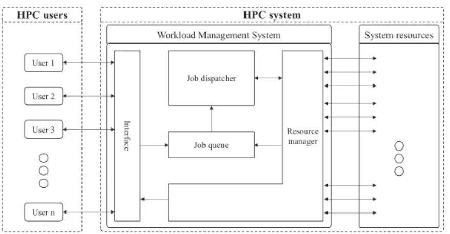
In Figure 1.3 we can see the typical basic software architecture used in mod-ern HPC systems. The components we will now present are part of the

Workload Management System, which is the component regulating the use

of physical resources in the system, and the one we are most interested in.

User Interface Users interact with the system through a software

inter-face, which acts as a frontend. This interface allows jobs to be remotely

submitted by users, and regulates their arrival and execution; besides, it will also allow users to track their status, and manage them. It could be either a

GUI-based or command-line interface. An HPC system usually also has one

or more queues for jobs submitted by users that are waiting to be executed, with different priorities and features.

Dispatcher Actual management of jobs is handled by the dispatcher

com-ponent, which periodically selects one or more jobs from the queues, and allows them to start on the system, either in a reactive or proactive way. The dispatcher includes the scheduler and allocator components, which re-spectively define the when and where of each job’s execution. In detail, the scheduler decides when a job should be executed, thus imposing the ordering

(21)

of jobs in the queue. The allocator, instead, decides which resources and computing nodes in the system a job should use. In general, the dispatcher component is the one responsible in the system with ensuring a good Quality

of Service (QoS) level, by minimizing the waiting times for the submitted

jobs. Besides deciding which, when and how jobs should run, the dispatcher is also tasked with triggering the start of these jobs by interacting with the

resource manager component.

Resource Manager The dispatcher is able to start jobs and allocate them

on specific nodes thanks to an abstraction layer called the resource manager: this entity keeps track of the state of resources and nodes in the system, besides that of running jobs. The resource manager usually acts as a server, with a monitor-like client running in each node in the system. Thus, when the dispatcher wants to execute a job, it will interact with the resource manager in order to perform scheduling and allocation, and then again to physically allocate the resources needed for the new job.

(22)

Chapter 2 Dispatching in HPC Systems

In this Chapter we will analyze the dispatching problem in HPC system, and see how it can be formalized. We will also discuss which are the most commonly used techniques and algorithms, and we will present some of the commercial solutions available on the market.

The Chapter is organized as follows: in Section 2.1 we will lay the formal foundations for the dispatching problem. In Sections 2.2 and 2.3, instead, we will discuss the scheduling and allocation sub-problems, respectively. Finally, in Section 2.4 we will look at the main commercial solutions for dispatching in HPC systems that are available in the market.

2.1 The Dispatching Problem

2.1.1 Formal Definition of Job

A job is, generically, a user-submitted task that is to be executed on an HPC system. Jobs in most HPC systems belong to the parallel class, and are composed of many independent running units that can communicate with each other, for example through message-passing interfaces [7].

A job J, made of an executable file together with its arguments and input

(23)

2.1. THE DISPATCHING PROBLEM

to it. Some of them are related to time, and the most important are:

• Jq: the queue in the system to which the job was submitted;

• Jtq: the time at which the job was submitted to the system;

• Jts: the time at which the job started its execution;

• Jte: the time at which the job ended its execution;

• Jde: the expected duration for the job, which is an estimation and not

representative of the real duration;

• Jdr: the real duration for the job, which is computed after its

termina-tion as Jte − Jts;

• Jdw: the wall time, which is the maximum time for which the job is

allowed to run, and usually determined by the system itself;

A job may have other descriptive attributes, such as the name of the user that submitted it. There also are some attributes specifically associated to the resources requested by the job and supplied to it: a resource is the most elementary hardware unit of a certain kind available in a computing node, like a CPU core, or a certain quantity of RAM. These attributes are:

• Jn: the number of job units requested by the job. These can be

consid-ered as the independent instances, each of them running on a specific node, that make up the job;

• Jr: a data structure representing which types of resources are needed by

each job unit, and in which amount. A job unit request is homogeneous

if all Jn units request the same type and amount of resources, and

heterogeneous otherwise;

• Ja: the resource assignation given by the system for the job, when it is

scheduled to start. It can be interpreted as a vector of Jnrecords, with

each of them containing the list of resources in a specific node assigned for a particular job unit.

(24)

According to how they behave in regards to the resources supplied by the system, we can additionally define various classes of jobs [7]:

• Rigid: these jobs need the exact amount of resources that were re-quested in order to run, and cannot adapt to any kind of change in their amount, either at run-time or at scheduling time;

• Evolving: unlike rigid jobs, they may request on their own initiative new resources to the system at run-time. If such new resources are not supplied by the system, the job won’t be able proceed;

• Moldable: these jobs can adapt to an amount of resources supplied by the system that is higher or lower than the requested one; after the jobs starts, however, such allocation of resources is never allowed to change again;

• Malleable: they are a generalization of moldable jobs, and admit changes in the allocation of resources in respect to the requested ones both at run-time and at scheduling time.

Practical Assumptions

Job unit requests in PBS-based systems like Eurora, presented in Section 3.1,

are all bound to be rigid and homogeneous, using Jn resource-wise identical

job units. Since this is a reasonable assumption, and Eurora is our system of interest, we will also adopt this constraint, which has nothing to do with the

heterogeneity of the underlying HPC system. Under this assumption, the Jr

structure will be a list, with each element Jr,k in it defining the amount of

resources for type k needed by each job unit.

Also, the system’s behavior regarding the wall time Jdw may differ according

to its nature: again, as in Eurora, we will suppose that any job exceeding in duration its wall time value will be terminated by the system.

(25)

Definition of Workload

Workloads are a very important part in the analysis of HPC systems. A

workload is simply a set of jobs relative to a certain time frame, that need to be dispatched according to their submission time values and resource re-quests. A workload may be synthetic, and thus generated statistically by software, or extracted from log traces belonging to a real HPC system. In both cases, the jobs’ real durations are included, allowing the workload to be used in simulated environments. Also, being inherently static, a workload allows for repeatable experiments and for reliable comparisons between mul-tiple dispatching techniques. A workload is usually stored in a text-like file, with a certain format and specific attributes, with each entry corresponding to a single job.

2.1.2 Formal Definition of Dispatcher

The dispatcher is a software component in online HPC systems, which selects pending jobs from the queue, and allows them to start their execution. For simplicity, we will consider a system with only one queue available, but our considerations will be valid for systems with multiple queues as well. A dispatcher should be very fast and not computationally intensive, as it is the component responsible for guaranteeing a good QoS level in the system, and it can negatively impact its performance. The dispatcher is part of the Workload Management System, and it may behave in two different ways:

• Reactive: the dispatcher is invoked only when significant events occur in the system and trigger a status change, such as when new jobs arrive on the queue, or some others terminate;

• Proactive: the dispatcher is invoked independently from events in the system, for example in a slotted manner, thus dispatching jobs in the queue at regular time intervals.

(26)

The basic behavior of a dispatcher is shown in Equation 2.1. The dis-patcher, when invoked, will allow a subset D of jobs waiting for execution in

the queue Q to start. For each job Ji of D, the dispatcher will have assigned

to it a starting time Ji

ts and a resource assignation J

i

a. This assignment is

called a dispatching decision, and jobs in D that were scheduled to start at the current time step are prepared and removed from the queue.

In a dispatcher, the scheduler and allocator components can be identified:

the scheduler is tasked to determine the starting time Ji

ts of each job in D and

is identified by the s function, which may depend on both the characteristics

of job Ji_{, and the status of the queue Q. The allocator, instead, defines a}

suitable resource assignment Ji

a for each scheduled job, and is identified by

the a function, again depending on both the job Ji and the queue Q. Both

the scheduler and the allocator interact with the resource manager compo-nent introduced in Section 1.4, in order to obtain information regarding the system’s status.

D = (J1, J2, ..., Jn) ⊆ Q

J_ti_s = s(Ji, Q), J_ai = a(Ji, Q) ∀Ji ∈ D (2.1)

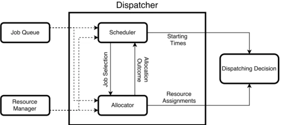
The three phases of dispatching, namely job selection, scheduling and

al-location are not to be intended in a sequential order. The subset D of jobs

that are successfully dispatched is actually determined after the scheduling and allocation phases. In general, a feedback loop is present between the three parts of dispatching: the scheduler may select a particular subset of jobs to dispatch depending on its job selection heuristics, with certain start-ing times, and pass them to the allocator. However, the allocator may not be able to find suitable assignations for certain jobs, forcing the scheduler to select another strategy, or a different subset of jobs altogether.

The reasoning we presented is synthesized in Figure 2.1. In this figure, the solid lines represent the flow of execution, while dashed lines represent infor-mation used by entities in the dispatcher.

(27)

Figure 2.1: A representation of the workflow for a simple dispatching system.

2.1.3 Metrics for the Evaluation of Schedules

In this section we will present some of the many metrics generally used to evaluate the effectiveness of a dispatcher. These metrics consider different factors, and cover various aspects of the system: by using combining them, we can obtain a detailed view of the dispatcher’s behavior, and make reasonable comparisons. As anticipated, a dispatcher is usually tested with a workload in order to evaluate its performance. This kind of methodology is preferable, as it allows for reliable and repeatable experiments.

All of the metrics we will present are mainly comparative: if a dispatcher achieved bad performance on a certain workload, it wouldn’t necessarily mean that the dispatcher itself is not effective, but most likely that the workload is inherently difficult and hard to manage. At the same time, by using the same workload we can effectively compare various dispatching methods. Finally, as most of the following metrics are computed on a job or

per-step basis, it is usually necessary to look at their distribution for a given

workload in order to obtain meaningful data on the system’s behavior. Makespan

The makespan is a temporal metric, and is very common for the evaluation of scheduling systems. It is formulated as follows:

(28)

2.1. THE DISPATCHING PROBLEM mks = max 0≤i≤n−1(J i te) −_{0≤i≤n−1}min (J i ts) (2.2)

As represented in Equation 2.2, the makespan expresses the time interval between the earliest starting job, and the latest ending job. It is, in other words, an estimation of how effectively a dispatcher can pack jobs by assign-ing them to resources in the system: lower makespans signify better results, as it means the dispatcher is able to efficiently use the resources available in the system, which will be busy for a shorter time.

The makespan metric, however, is meaningful only for batch systems, that are bound to run for finite amounts of time; for online systems, instead, which are by definition made to be ever-running and prone to continuously-changing work conditions, the makespan is less relevant and not important.

Waiting Time

The waiting time is a temporal, per-job metric, and as the name implies it can be expressed through the following formula:

waitJ = Jts − Jtq (2.3)

As it can be seen in Equation 2.3, the waiting time for a job corresponds

to the time interval between its arrival in the queue, expressed by Jtq, and

its starting time, represented by Jts. In general, lower waiting times can be

associated with better results, as the system is able to promptly dispatch jobs without having them to wait too much time in the queue.

Sometimes, for systems with multiple job queues each with a different priority and expected waiting time, it may be useful to consider a normalized form of the waiting time, which is the tardiness: this metric corresponds to the job’s wait divided by the expected waiting time for its queue, and is an approximation of the job’s relative delay compared to how much it would have been expected to wait before being started.

(29)

Slowdown

The slowdown metric can be seen as a refined form of the waiting time [8]. The waiting time, in fact, does not consider one important fact: jobs with long durations are less susceptible to high waiting times, as they will have

lower influence on the total turnaround time, represented by waitJ + Jdr,

which is the sum between the waiting and the real execution times. On shorter jobs, instead, the turnaround time could easily become greater than the execution time by orders of magnitude. The slowdown metric captures this, and can be interpreted as a sort of perceived waiting time. It is formu-lated as follows:

sldJ =

waitJ + Jdr Jdr

(2.4) As expressed in Equation 2.4, the slowdown is computed as the turnaround time normalized by the real execution time of the job. A system achieving comparatively lower slowdown times is more performant: however, since the slowdown has a big impact on short jobs mainly, it is usually good practice to also consider the standard waiting time, which is equally representative for short and long jobs.

Throughput and Queue Size

The throughput and the queue size metrics are highly descriptive of a dis-patcher’s performance. These are not per-job metrics, but rather per-step ones: this means they are computed every time the dispatcher is invoked to schedule new jobs. The queue size and throughput metrics can be expressed through the following equation:

tpt= |D|

qst= |Q|

(2.5) Equation 2.5 can be interpreted in a straightforward way. The throughput

(30)

and started at a certain time t, as seen in Equation 2.1. The queue size qs, instead, corresponds to the size of the queue Q after dispatching has been performed. As said earlier, both metrics are computed for every time step t in which the dispatcher is invoked. Also, the two metrics behave similarly: an higher throughput corresponds to a lower queue size, both of which mean the dispatcher is able to schedule jobs effectively. Considering just one of the two is usually enough to evaluate the performance of a system.

Resource Utilization

The most generic metric for the evaluation of a dispatcher in an HPC system is the resource utilization: it consists in the amount of resources in the system that are actively used by jobs at every time step. This is a per-step metric as well, but in this case we are considering all time steps, and not only those in which dispatching is involved. This is because jobs terminate their execution and free resources in the system independently from the dispatcher. A simple way to compute resource utilization is the following:

loadt=

Rused

Rtotal

(2.6) The formula depicted in Equation 2.6 defines the load ratio at time t,

which is the ratio between the amount of used resources Rusedin the system,

and the total amount Rtotal of those available by default in it. This is a

very good way to express the resource utilization, since the load ratio is represented by a number bounded in the range [0, 1], thus independent from the scale of the system.

It is common to consider a specific subset of resource types in the system, in order to obtain more comprehensible and meaningful results: because of this, resource utilization is often computed in regards to CPU resources alone, since they are the most common ones and usually needed by all jobs.

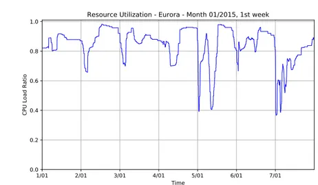
In this case, looking at the distribution of resource utilization values may not be informative: using a visualization in function of time is much better,

(31)

2.1. THE DISPATCHING PROBLEM 1/01 2/01 3/01 4/01 5/01 6/01 7/01 Time 0.0 0.2 0.4 0.6 0.8 1.0

CPU Load Ratio

Resource Utilization - Eurora - Month 01/2015, 1st week

Figure 2.2: A plot depicting CPU resource utilization for the Eurora system, in the first week of January 2015.

and allows us to better compare different dispatching methods, as seen in Figure 2.2. The explanation is that the resource utilization metric is not meaningful at all times: during its normal operation, an HPC system will cross many working phases, some of which are not relevant. We are not, in fact, interested in periods when the system is in an idle or low-utilization state. We are only interested in observing the behavior of the system when it is almost fully loaded and there is a constant stream of jobs being submitted, as only in this scenario the qualities of a particular dispatcher can arise.

In general, low average resource utilization values and long queues in-dicate fragmentation in the system: with this term we mean the condition in which some nodes have few resources left, that cannot be used by any job and are thus wasted, and is mostly caused by badly designed allocation heuristics. Conversely, a dispatcher able to keep the system’s resources fully loaded at most times is usually very good.

Resource Allocation Efficiency

Resource allocation efficiency is a metric that can be used to evaluate the

(32)

2.2. THE SCHEDULING SUB-PROBLEM

per-job metric, and is formulated as follows: ef fJ = Jn∗ P k∈res Jr,k P i∈Ja Ravl(i) (2.7)

In Equation 2.7, the upper member in the fraction represents the total

amount of resources needed by a job, with Jnbeing its job units, and Jr,k the

amount of resources of type k needed by each of them. Ja is instead the list

of distinct node assignations for job J, and Ravl(i)is the amount of available

resources in such nodes before dispatching.

The resource allocation efficiency allows us to estimate how efficiently a dis-patcher can allocate jobs in the system: high values indicate that a job uses few nodes, and that these nodes are used to their fullest, leaving no free resources, and thus also implying low fragmentation. An highly effi-cient dispatching system will lead to higher throughput, and to lower power consumption as well.

This metric can be formulated on a per-step basis as well: in this case, at each time step all the running jobs and the nodes on which they are allocated are considered. This variant of the resource allocation efficiency metric is mostly related to the system utilization over time, and can be seen as a refined form of the load ratio.

2.2 The Scheduling Sub-Problem

2.2.1 Definition and Hypotheses

In HPC systems, the scheduling problem consists in assigning starting times

Jts to a series of jobs, by using heuristics in order to maximize the resource

usage of the system, and minimize the waiting times. At this stage we are not assigning resources to jobs, but only determining, if necessary, wether they fit the current available resources in the system or not: which of those will be assigned to them is up to the allocator to decide.

(33)

In general, there are two possible approaches to scheduling in HPC systems [10]. These are:

• Queueing: the scheduler will use a certain ordering criteria for jobs in the queue, and will try to schedule as many of them as possible every time the dispatcher is invoked, in a sequential order: hence, jobs are always given an immediate starting time, corresponding to when the scheduler made its decision. When the scheduler reaches a job that cannot be dispatched, because there are not enough available resources in the system, it will terminate, as not to violate the properties of the queue. This is the most common approach; it is also very simple, and not computationally complex.

• Planning: every time the dispatcher is invoked, the scheduler will try to compute a schedule plan for all jobs in the queue, or a subset of them; that is, a specific starting time is assigned to each job, without violating the system’s resource constraints. This is done in order to find the globally best possible placement for jobs, in terms of waiting times or other metrics, which simply cannot be done by a queueing-oriented scheduler. Unfortunately, planning-oriented scheduling algorithms are inherently complex, as the problem itself of assigning starting times to tasks with certain constraints belongs to the NP-Hard class [11]; besides, in order to compute such a schedule and obtain good results,

it is necessary to have reliable estimations Jde of the jobs’ length: this is

often not the case, and all we have is the wall time Jdw, which severely

over-estimates the job length and leads to resource waste.

Out of the two presented approaches, the queueing one is the most com-monly used in HPC systems, and in most commercial solutions for dis-patching. The planning approach, instead, while being potentially better is plagued by its computationally intensive nature, and thus more rarely used.

(34)

2.2.2 Common Scheduling Algorithms

In this section we will discuss the most common algorithms for scheduling in HPC systems. Please note that these methods all belong to the queueing-oriented kind, except the last one.

First-Come First-Served

The first and most simple scheduling algorithm we will present is First Come

First Served (FCFS). As the name implies, this method does not impose any

kind of ordering on the job queue, and the scheduler will try to dispatch jobs in the order in which they arrived.

This algorithm has some qualities: first of all, as we mentioned earlier, it is very simple and computationally inexpensive. Also, since jobs are not artificially sorted, it ensures fairness in the scheduling process, and it is not possible for some jobs to suffer starvation. Finally, it does not need any kind of information about the system or the jobs in order to perform its dispatching decisions. However, since no kind of optimization is performed, FCFS may pick jobs in a highly sub-optimal order, thus leading to bad performance, low resource usage in the system, and long waiting times.

Longest Job First and Shortest Job First

The Shortest Job First (SJF) and Longest Job First (LJF) algorithms are the natural evolution of FCFS. In simple words, these two methods will sort jobs in the queue by using their estimated duration in ascending (SJF) or descending order (LJF). These are slightly more computationally expensive than the FCFS algorithm, however the computational cost can be reduced by maintaining the job queue in a sorted state between dispatching calls. The choice between SJF and LJF is not obvious, and mainly depends on the kind of workload the system is subject to. However, among the two, SJF is usually the most robust choice, and leads to good results in terms of throughput and waiting times, despite being very simple.

(35)

Unfortunately, these two algorithms still have some issues to be considered: first of all, since sorting is explicitly performed on the job queue, we must consider the possibility of starvation for some jobs. For example, in a system employing SJF where the frequency of short jobs is very high, a long job may end up waiting indefinitely in the queue. Secondly, both methods need an

estimation Jde of the jobs’ length in order to perform sorting: if there is not

one available, the wall time Jdw must be used, leading to worse results.

Priority Rule-Based

Priority Rule-Based (PRB) scheduling is a generalization of the FCFS, SJF

and LJF algorithms seen before [12]. It still uses a simple queueing-oriented approach, but in this case the sorting criteria for the jobs is a generic priority

rule that can be changed and tuned according to the users’ needs and the

system’s type. For example, in a system with multiple job queues, each with a specific priority and expected waiting time, a priority rule could be based on a job’s tardiness, introduced in Section 2.1.3 [7].

As with the methods we have seen before, caution must be taken while de-signing new priority rules: the risk of favoring certain classes of jobs while compromising others, with certain workload distributions, is always present. Backfill

Backfill is a very commonly used queueing-oriented scheduling technique,

and is an industry standard in HPC systems. Generally speaking, backfill is not a technique made to replace the heuristics we have presented so far, but rather it can be placed on top of them, as it does not make any assumptions on job ordering.

In a standard scheduling algorithm, like the ones we have seen earlier, jobs are scheduled in a sequential manner depending on the queue’s ordering. This is what we would call the normal mode of the scheduler. Whenever the allocation for a job fails, the scheduler terminates, and returns the set of jobs

(36)

Figure 2.3: The representation of a schedule produced by an Easy backfill algorithm. Image taken from [13].

that it managed to schedule. In a backfill scheduler, instead, the procedure does not terminate when a job cannot be allocated: instead, a reservation is made for it. Specifically, the algorithm will scan through the set of currently

running jobs, and from their estimated duration Jde it will compute the

earliest starting time in which enough resources will be available in order to start the blocked job. Then, a set of resources in the system is reserved for that specific starting time and for the job’s expected duration.

As long as the reservation has not been fulfilled, the scheduler operates in the homonymous backfill mode: in this special mode, the scheduler will try to dispatch jobs in the queue other than the blocked one, as long as they do not interfere with the reservation; in particular, they must not use any of the resources in the reserved set, in the time frame of the blocked job’s planned execution. Also, in backfill mode the scheduler is allowed to skip jobs in the queue that cannot be dispatched.

What we just described is the basic functioning of the backfill algorithm. There are, however, two different variants of this technique:

• Easy Backfill: only one reservation at most is maintained at any time. This reservation corresponds to the blocked job, which is located at the head of the queue;

(37)

• Conservative Backfill: multiple reservations are admitted, and cre-ated whenever a job cannot be scheduled. In this case, there is no real functional distinction between the normal and backfill modes.

It has been shown that there is no clear winner between the two Backfill modes, and their behavior mainly depends on the kind of workload they are subject to [13], even though Conservative is much more complex than Easy Backfill. In Figure 2.3 a representation of how Easy backfill works can be

seen, with J2 _{being the blocked job.}

Finally, it must be said that since backfill relies on estimations for the jobs’ length, its performance heavily depends on these: in fact, an overestimation of the jobs’ length might lead to wasted resources in the backfill interval, while an underestimation could lead either to preemption of the jobs that didn’t manage to finish before the end of the backfill interval, if the system supports it [14], or to a delay of the reservation itself.

Optimization and Planning-Oriented Algorithms

In this last section we will look at how the scheduling problem can be for-mulated in order to pursue an optimization and planning-oriented approach. In general, an algorithm of such kind will operate on a subset of the job queue of fixed maximum size, which will be sorted according to some priority rule. As mentioned earlier, for these jobs a schedule plan is computed, detailing the starting times for each one of them. As such, this is the only case in which the subset D of jobs that are to be dispatched is determined before the scheduling procedure.

In order to formalize the problem, we will now define its parameters:

• Variables: the starting times Jts for jobs in the subset D of the queue

being considered;

• Constraints: the schedule plan must never violate the system’s re-source availability constraints;

(38)

2.3. THE ALLOCATION SUB-PROBLEM

• Objective Functions: a certain metric that is to be minimized in or-der to obtain an optimal solution, such as the makespan or the average

waiting time.

This is a general characterization for the scheduling problem, which is valid for most applications in HPC systems. Having defined its parameters, a method for solving the problem has to be chosen: since it belongs to the NP-Hard class, exhaustive search must be excluded from the viable alterna-tives, as it would be unfeasible on an online system. Besides, a sub-optimal solution is often more than enough for this kind of task. As such, optimiza-tion techniques like simulated annealing, genetic optimizaoptimiza-tion, tabu search or

constraint programming are much preferable. In general, these techniques

can be adapted to the timing constraints of the system by applying temporal limits to the search, with better solutions more likely to be found as the search time is increased.

As we have seen with the previous algorithms, being able to correctly estimate the jobs’ length is critical: wrong estimations will result in the computed schedule plan to not be respected, thus worsening the performance of the algorithm. At the same time, an approach must be defined in regards to new jobs arriving in the queue. The algorithm might be designed to preserve an already-computed schedule plan, and fit the new jobs inside it at the next dispatching call. Conversely, it might be preferable to recompute the schedule plan from scratch every time, leading to potentially better results but also to an higher computational cost. An algorithm belonging to this class will be described with great detail in Section 5.2.4.

2.3 The Allocation Sub-Problem

2.3.1 Definition and Hypotheses

In this section we will treat the allocation sub-problem in dispatching. This

(39)

units Jn and resource types Jr, to jobs in the subset D of the queue that

were selected by the scheduler and given a starting time.

Allocation is a task of great importance in an HPC system. Good alloca-tion policies allow to greatly improve parameters of the system like power consumption and average temperature, but also allow for lower resource frag-mentation and, in turn, lower waiting times.

We can distinguish between two main approaches for allocation in HPC sys-tems [15]:

• First-Fit: this approach is similar to queueing-oriented scheduling. In this case, jobs are allocated one by one separately, in the order specified by the scheduler. For each job, resources are picked from a list of nodes, which is sorted according to a certain criteria: the algorithm will pick resources from the list while traversing it, until the job’s request has been satisfied. Usually, the algorithm will try to fit as many job units as possible in each selected node. If the algorithm reaches the end of the list without finding enough resources, the allocation is considered as failed, and the scheduler must then decide how to proceed;

• Mapping: conversely, this approach is equivalent to planning-oriented scheduling. Here, jobs in D are considered as a whole and collectively allocated, using complex algorithms that try to optimize specific met-rics [15]. Like the scheduling problem, also the mapping problem, which consists in assigning resources to a given set of jobs in an optimal man-ner, belongs to the NP-Hard class. Besides, most mapping methods are made to be used on their own, without depending on a scheduler, as they can decide the jobs’ starting times as well: in these cases, our proposed architecture for a dispatcher, seen in Section 2.1, is not ap-plicable.

In most HPC systems, allocation algorithms belonging to the first-fit class are used. Mapping algorithms, while potentially better, are also much more complex, and usually need specialized software architectures in order to be

(40)

correctly integrated with scheduler algorithms. For these reasons, we will not further discuss mapping algorithms.

2.3.2 Common Allocation Algorithms

In this section we will present some allocation methods that fall into the first-fit category, and are very commonly used in HPC systems. Most of the algorithms in this section perform a fail-first search: this means that the ordering of nodes is such that a suitable allocation is more likely to be found on later nodes in the sorted list, rather than the first ones. This is due to the fact that such type of search, while theoretically more expensive than a success-first one, usually allows for better results.

Simple First-Fit Policy

The first algorithm for allocation we will present is the simple first-fit pol-icy: similarly to the FCFS scheduling policy presented in Section 2.2.2, this method does not perform any kind of sorting, and nodes are scanned for available resources in their default order. This order may be numerical or lexicographical basing on each node’s ID, but it may also be a static ordering made to improve certain performance parameters.

While simple, this algorithm has not inherently bad performance; it is in fact very common in HPC systems. It also has a few interesting properties: since nodes are always scanned in the same order for all jobs, the system’s resources will statistically be filled in an incremental manner. This means that before moving to the next nodes in the list, the previous ones will usually have reached maximum load, leading in turn to low resource fragmentation. Best-Fit Policy

The best-fit heuristic is an improvement over the basic first-fit allocation method. In this case, nodes in the system are actively sorted according to the amount of resources available in them, in ascending order. This means

(41)

that the first elements in the nodes’ list will usually correspond to ones that have none or very little available resources.

The purpose of this is to decrease fragmentation in the system and thus perform consolidation. The first-fit policy is not enough for this, as jobs will terminate and release their resources in arbitrary order, which means that, when the system is fully loaded and running, the allocator’s performance may become completely random. The best-fit policy addresses this, ensuring that at every allocation the best-fitting nodes are selected, keeping fragmentation low.

For complex, sorting-based allocation algorithms like best-fit performance may be a concern: systems may in fact scale horizontally indefinitely, and could be made of thousands of nodes. Performing sorting on the nodes’ list at every allocation is thus not very efficient. To address this, there usually are two possible ways: a persistent, sorted list of nodes in the system may be kept, which will drastically decrease the computational cost of the algorithm; in alternative, smaller subsets of nodes in the system may be considered for allocation, by using for example tree-based selection techniques.

Priority Rule-Based

As we have seen with the scheduling problem, there also exists a priority

rule-based generalization for allocation algorithms. In this case, the order of

nodes in the system picked for allocation depends on a user-defined priority rule, which may take several factors into account. Again, the development of priority rules is not a trivial task, and without mindful design it can lead to badly performing allocators.

Such an allocation heuristic, for example, may be related to heterogeneous systems equipped with multiple accelerator types: a priority rule could weight different resource types, assigning greater weight to those that are scarce in the system and not available in every node, in order to not penalize jobs that actually need them. The nodes containing such resources would then

(42)

be statistically placed towards the end of the nodes’ list, thus preserving the critical resources.

Cooling-aware and Power-aware Placement

Some allocators in the literature are aimed at minimizing the system’s

tem-perature and cooling power [16]. Cooling systems are in fact a very important

component in HPC systems, and managing to keep the overall system tem-perature low will lead to better performance and to more efficient power con-sumption. These techniques go under the name of cooling-aware placement, and it is estimated that, in an optimal scenario, the use of such algorithms can reduce the costs for environmental management in an HPC system by up to 30% [17].

Minimizing the overall system’s temperature increase after the allocation of a job implies the use of complex optimization and heuristic techniques, besides models for temperature prediction in specific parts of the system. Also, in order to keep track of the system’s temperature in all nodes, an additional hardware-software infrastructure is necessary.

Having said this, such a type of allocation is usually obtained by placing jobs in nodes that are physically far from each other, in order to evenly distribute the temperature increase; in fact, placing all job units in nodes close to each other would cause a spike in the temperature for that area, which would require higher cooling power.

Cooling-aware placement can help reduce overall power consumption: however, that is often not enough, and specialized power-aware placement techniques are needed. As we have seen, the first-fit and best-fit algorithms are able to keep fragmentation in a system low: this is a good starting point for power consumption optimization, as having nodes either in a fully loaded or idle state is an ideal condition. This way, many nodes are able to enter special, low-power idle modes, that can drastically improve the overall energy efficiency.

(43)

2.4. COMMERCIAL WORKLOAD MANAGEMENT SYSTEMS

Similarly to what we have seen with cooling-aware placement, there are com-plex power-aware placement algorithms, which try to minimize the overall power consumption increase after the allocation of a job [18]; again, complex models for power consumption prediction in regards to the system’s hardware components must be used.

Topology-aware Placement

Often the physical placement of a job, independently from the resources available in its assigned nodes, may have a big impact on its performance. Parallel jobs, in fact, usually have intricate communication patterns: this means that the farther away job units are placed from each other, the more network hops are needed for communication. This implies higher network strain and latency times, which both lead to worse performance on the job’s side, and higher power consumption. For this reason, some allocation meth-ods try to place units of the same job in a physical area as small as possible, trying to improve the locality of a job.

In order to perform this kind of allocation, it is necessary to know the topology of the system. Many such algorithms are known in literature [19], and the allocation policy used in Slurm also exploits locality [20]: these methods map nodes in a tree, with each level signifying different grouping hierarchies for nodes. Leaf nodes sharing the same parent generally belong to the same basic grouping unit, which may be a rack or a cabinet. This kind of approach allows for efficient tree-based search techniques, and is most effective on large-scale systems.

2.4 Commercial Workload Management Systems

In this section we will present some of the most famous commercial HPC Workload Management Systems, and their peculiarities.

(44)

2.4. COMMERCIAL WORKLOAD MANAGEMENT SYSTEMS

The first solution we are looking at is Slurm [20], which is a free, open source HPC dispatching system targeted for Linux/Unix. Slurm is main-tained on GitHub, and has an active community behind it. Due to its highly modular and customizable nature, Slurm is used in roughly the 60% of HPC systems in the world, including the Tianhe-2 system introduced in Section 1.3. Besides job scheduling and resource management, Slurm has many other features, mainly for system monitoring and control. It is advertised as an highly scalable system and as easy to configure, thus useful in many contexts. Slurm uses a topology-aware allocation policy, trying to improve locality and resource utilization, and supports heterogeneous job unit requests as well.

The second WMS we present is Portable Batch System (PBS) [21], which is a commercial product made by Altair. This is the dispatching system also used in Eurora, and is an highly reliable product that has been on the market for 20 years in different iterations, even though originally it was free and open source. Many other products in the market are based on PBS, such as Torque, which we will describe later. Compared to Slurm, PBS has also power-aware capabilities, however it is far less modular and harder to customize. Unlike the former, PBS also does not support heterogeneous job

unit requests, which means a PBS job is limited to having Jn homogeneous

job units, each requiring the same amount and type of resources.

Torque [22] is a WMS based on the original open-source PBS project.

It is produced by Adaptive Computing, but is free and open source, with the company being tasked with user support and development. Similarly to Slurm, Torque is highly modular, scalable and customizable, and can be adapted to a great variety of systems, with a focus on heterogeneous ones. At last, we will talk about the Maui system [23], which is right now also under the custody of Adaptive Computing. Maui is mostly a predecessor to modern dispatching systems, and was mainly developed during the 90s. It provided customizable fairness, job priority and allocation policies, which are a standard in modern products. It is now discontinued, and its core was inherited by the Moab system, now still actively developed.

(45)

Chapter 3 The Eurora System

In this chapter we will introduce the Eurora system, which was chosen in order to evaluate the various dispatching methods that will be presented later. We will analyze a workload from Eurora as well, in order to better understand its usage patterns, and finally we will discuss some methods to estimate the jobs’ durations on such workload.

The chapter is structured as follows: in Section 3.1 we will introduce the Eurora system, and its main features. In Section 3.2 we will then analyze the workload from Eurora that will also be used for testing later in the thesis. Finally, in Section 3.3 we will discuss a data-driven method for the estimation of the jobs’ durations in the workload.

3.1 System Overview

Eurora is a prototype HPC system built in 2013 by CINECA in Bologna,

Italy, in the scope of the Partnership for Advanced Computing in Europe (PRACE) [24], and is pictured in Figure 3.1. It is a small-scale HPC system with an hybrid architecture, designed for low power consumption: Eurora was in fact listed as #1 in the Green500 list of Top500, which ranks the most efficient HPC systems worldwide, in July 2013 [2]. It could achieve a 3.2 GFlops/W computing power, and had a peak power usage of 30.7KW.

(46)

3.1. SYSTEM OVERVIEW

Figure 3.1: A picture of the Eurora system. Image taken from [24]. The Eurora system is a heterogeneous cluster made of 64 nodes: each of these nodes has two Intel Xeon SandyBridge CPUs with 8 cores, 16GB of RAM, and 100TB of disk space. Additionally, each node has two accelerator units available: specifically, 32 nodes are equipped with two NVIDIA Tesla K20 GPUs, while the remaining 32 are equipped with two Intel Xeon Phi

Many-Integrated-Cores (MIC) units. Some nodes differ slightly in terms of

CPU and RAM: one half of the nodes, in fact, uses CPUs clocked at 2.0Ghz, while the other half uses CPUs with a clock of 3.1Ghz. At the same time, 6 nodes in the system, with the higher performance CPUs, mount 32GB of RAM storage instead of 16.

The system’s network has the topology of a 3D torus, and networking tasks in each node are handled by an Altera Stratix-V FPGA unit and by an InfiniBand switch operating in Quad Data Rate mode. InfiniBand is a stan-dard for computer networking with very high throughput and low latency, and is commonly used in HPC systems [25].

The nodes run a Linux CentOS 6.3 distribution, and the workload man-agement system being used is Portable Batch System (PBS), which employs various heuristics for optimal throughput and resource management; since

(47)

3.2. ANALYZING THE EURORA WORKLOAD

Queue Max. Nodes Max. Cores/GPUs Max. Time Approx Wait debug 2 32 / 4 00:30:00 Seconds parallel 32 512 / 64 06:00:00 Minutes longpar 16 256 / 32 24:00:00 Hours

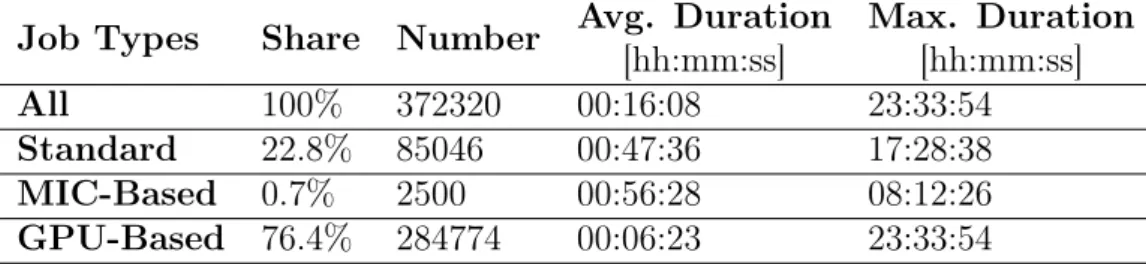
Table 3.1: The constraints related to each of the job queues in Eurora. PBS is being used, jobs in Eurora are limited to homogeneous job unit re-quests, as mentioned in Section 2.4. Additionally, Eurora uses three different queues for job dispatching [7], named debug, parallel and longpar, with dif-ferent priorities and resource constraints. The debug queue is designed for quick, small jobs executed for debug purposes; the parallel queue is instead designed for ordinary jobs, while the longpar queue is made for long, low priority jobs that are to be scheduled during the night. The specifics for each queue can be seen in Table 3.1.

The heterogeneity seen in the available resources grants great flexibility to Eurora, and also makes it an interesting system to analyze, especially due to its limited scale. In such a context, the dispatcher component has primary importance, in order to make good use of the system: for these reasons, Eurora will be the object of our analysis in the scope of new dispatching heuristics development.

3.2 Analyzing the Eurora Workload

We will now consider a workload extracted from Eurora’s log traces, and analyze it thoroughly from different points of view. The workload will be used for testing later in the process, with the AccaSim simulator that will be presented in Chapter 4.

3.2.1 Workload Overview

The workload is made of 372320 jobs and covers one year of data, from April 2014 to June 2015. As mentioned earlier, in Eurora there are GPU and

Development of Data-Driven Dispatching Heuristics for Heterogeneous HPC Systems

Alma Mater Studiorum · Università di

Bologna

DEVELOPMENT OF DATA-DRIVEN

DISPATCHING HEURISTICS FOR

HETEROGENEOUS HPC SYSTEMS

Relatore:

Chiar.mo Prof.

Ozalp Babaoglu

Correlatore:

Chiar.ma Prof.ssa

Zeynep Kiziltan

Presentata da:

Alessio Netti

II Sessione

Anno Accademico 2016/2017

Introduzione

Introduction

Contents

List of Figures

List of Tables

Chapter 1

An Overview of HPC Systems

1.1

HPC Systems and their Purposes

1.2

Taxonomy of HPC Systems

1.3

State of the Art

1.4

Typical Structure of an HPC System

1.4.1

Physical Architecture

1.4.2

Software Architecture

Chapter 2

Dispatching in HPC Systems

2.1

The Dispatching Problem

2.1.1

Formal Definition of Job

2.1.2

Formal Definition of Dispatcher

2.1.3

Metrics for the Evaluation of Schedules

2.2

The Scheduling Sub-Problem

2.2.1

Definition and Hypotheses

2.2.2

Common Scheduling Algorithms

2.3

The Allocation Sub-Problem

2.3.1

Definition and Hypotheses

2.3.2

Common Allocation Algorithms

2.4

Commercial Workload Management Systems

Chapter 3

The Eurora System

3.1

System Overview

3.2

Analyzing the Eurora Workload

3.2.1

Workload Overview