A novel distributed approach to power control in wireless cellular networks

(1)

POLITECNICO DI MILANO

Dipartimento di Elettronica, Informazione e Bioingegneria Master Program in Automation and Control Engineering

A NOVEL DISTRIBUTED APPROACH TO POWER

CONTROL IN WIRELESS CELLULAR NETWORKS

Supervisor: Prof. Maria Prandini Co-supervisors: Prof. Kostas Margellos

Alessandro Falsone, MSc

Stefano Mutti, 823466

(2)

(3)

Abstract

In this thesis, we address power control in a wireless cellular network. More precisely, mobile users in the network communicate with the base station in their cell. The base station has to set the transmission power of all users in its cell so as to optimize the quality of communica-tion. Interference due to communication of users on the same wireless channel is coupling the decisions of all base stations in the cellular network. Here, we propose a distributed al-gorithm based on proximal minimization that makes the base stations reach consensus to a solution optimizing the signal to interference plus noise ratio. The performance of the pro-posed approach is compared with that of an alternative gradient-based distributed approach via an extensive simulation study.

(4)

(5)

1 Introduction

Power control in wireless cellular networks has been attracting a lot of attention in the latest decades, due to the pervasive use of wireless communications, [6, 16].

The large growth of the number of wireless devices has prompted the need of introducing suitable resource management strategies so as to allow high quality of transmission while avoiding excessive power consumption. This latter aspect is critical for those devices that are using some battery and, hence, have limited autonomy.

Each cell in the network is associated with a base station and base stations exchange date via wired communication. Mobile users in the same cell are assigned to the same base sta-tion and exchange data with it via wireless communicasta-tion. If they all use the same wire-less channel, then their signal is interfering with those of the other devices in their same cell and in neighboring cells as well. This deteriorate the throughput of the device, since a lower Signal to Interference plus Noise Ratio (SINR) causes a larger number of retransmissions, and hence reduces the effective data transmission rate. Due to this common resource (the wireless channel) sharing, setting the transmission power of each device leads to a large op-timization problem involving all devices in the cellular network. Solving this opop-timization problem in a centralized way can be computationally challenging and also would require the transmission of much information between base stations, possibly overloading the commu-nication network.

As a matter of fact, most of the approaches proposed in the literature are based on a dis-tributed scheme and they can be classified into two main categories: autonomous and non-autonomous, the distinguishing feature being that, while in the former communications

(8)

oc-Chapter 1. Introduction

cur only between base station and mobile users, in the latter base stations collaborate and exchange information.

The approach described in [8] and further studied in [16], belongs to the first class and aims at minimizing the total power subject to constraints on the SINR via a distributed iterative algorithm. At every iteration, each mobile user sets its power, transmits at the current iterate power value, and then refines it based on the information on the SINR provided by its ref-erence base station. Autonomous distributed approaches to power control based on games between non-cooperative users are proposed in [1] and [7]. A further autonomous approach in the literature consists in formulating power control as an open loop global optimization problem where the SINR is not a constraint but has to be optimized via a distributed scheme, [11, 12].

The solution of the power control problem in a distributed but non-autonomous fashion in-volves communication between neighboring base stations and information sharing on their local solutions. Solving a problem in a non-autonomous way has its advantages: the ex-change of information between base stations can bring to a faster optimization and to a more robust scheme. In turn the additional communication overhead is not an issue since, typi-cally, base stations are connected via a wired backbone.

In this work, we propose a novel distributed non-autonomous algorithm for power control in a single channel wireless cellular network. The algorithm is derived from the proximal minimization based approach to distributed optimization recently introduced in [13]. In [15], the same problem is addressed via sub-gradient based distributed optimization, which is adapted here to our modeling set-up where multiple mobile users are possibly linked to the same base station.

Making a theoretical comparison between the two algorithms is difficult, and here we hence head for a numerical comparison via an extensive simulation study.

In summary, the contributions of this thesis are as follows:

• formulation of the power control problem for a single channel wireless cellular network where possibly multiple mobile users are communicating with the same base station;

• introduction of a distributed non-autonomous algorithm for power control which is derived from the proximal minimization based approach to distributed optimization;

(9)

and

• a comparative analysis via estensive simulations with an alternative method in the lit-erature derived from sub-gradient based distributed optimization.

(10)

(11)

2 Power control problem formulation

and proposed solution

2.1 Background

Nowadays wireless and radio communications rely on a wide range of technologies and pro-tocols , result of decades of work and research. This improvements brought speed , quality and reliability into networks but made also the models more variegate and complex to con-trol and optimize.

Creating a model of the network starts with the analysis of the cells and the channels, in fact a network can work using a single channel or more. Grids are usually composed of an hexag-onal or square cell pattern,this is due to the angular capability of the used antennas, which is 120° degree in the hexagonal one and 90° degree for the square.

Concerning the channels, a system can use a single channel for all the cells or a multi-channel method, in which a finite set of frequencies is fixed on alternate cells. A single channel is eas-ier to implement, especially if we consider scalable systems, but all the powers interfere each other because they use the same frequency. The other method is harder to implement but allows to have less interference cause the frequencies change between cells,hence the in-terference apply only between cells with the same frequency, in figure 2.1 is possible to see the comparison between a single channel network and a multi-channel one with frequency reuse.

This difference reflects on the SINR value of every connection, cause signals disrupt each other only if they use the same frequency.

Another parameter to take in account is the channel access method, which in this case is the Code Division Multiple Access, known as the CDMA. With the CDMA access method it is

(12)

pos-Chapter 2. Power control problem formulation and proposed solution

Figure 2.1: single channel on the left and multi-channel on the right

sible for a given number of mobile users to communicate and transfer data simultaneously on the same channel, this leads to interference between users in different cells and especially users in the same cells if two or more users are attached to the same base,hence to a decrease of the quality of service and to a worse connection.

For an extensive survey on CDMA based network refer to [17].

The environment upon which the simulations are done is a finite cellular wireless network with a number n of mobile users(MU ) and a number m of base stations(B S), the communi-cation between base and user are held on a common wireless channel.

We will assume the channel to be static and unique, like seen in the left part of 2.1. The links between Mobile users and stations are fixed, every MU is attached to the nearest B S, forming

n links. The connection protocol is based on pilot signals sent by the bases for informing all

the users of the relatives distances, after a user receives the signals from the reachable bases it attaches to the nearest one, for this reason some of the MU s may be communicating with the same B S.

The channel is assumed to be static , and the system to be fixed in time, the channel coeffi-cient between MUjand B Si is denoted by hi , j , and is assumed to be known only by B Siper

every mobile user.

In a wireless network the channel coefficients are measured by the bases using pilot signals, but for the simulation we need to use one of the numerous models provided by literature. In this work the channel coefficient decay is due only to the distance, it decays by the forth power of the distance and also includes the effects of shadowing.

(13)

2.2. Statement of the power control problem

The bases are connected each other with a reliable wired connection, every base is at least connected to another base. The set of bases connected to B Si is denoted by Ni, where every

base is also contained in its neighbors set.

The network is fully connected, which means that the information of every base can reach every other base in a finite number of iterations.

In figure 2.2 is shown a generic map with 4 bases and 10 users, the black dotted lines show the backbone links between bases, all the distances are expressed in kilometers.

Figure 2.2: Map with 4 bases and 10 users

The power control problem is that to select the optimal powers of the MU s in such way to optimize an objective function.

Different objective functions are available, every one focused on a different aspect of the con-nection or on different parameters [7]. In our case the objective function is related to the uplink throughput and the power consumption of the mobile users.

2.2 Statement of the power control problem

Let p be the vector of the powers, where the j-th element is the power used by MUj and its

values are constrained, and let n be the number of bases in the network.

Let hi , j be the vector of the channel coefficients between MUjand the base B Si, every base

(14)

Chapter 2. Power control problem formulation and proposed solution

Letσ2be the thermal noise, which afflicts all the bases in the same way. The SINR of MUjat B Siis defined as:

γj(p, hi) =

pjh_{i , j}2

σ2₊P

k6=jpkh2_{i ,k}

This quantity is strongly related to the quality of the base-user connections in the system, and hence to their performances and throughput. Let Uj be the utility function associated with

the SINR on link j , and nu(i ) the set of MUj attached to the B Si, the power control problem

is that to operate at the optimal point in the utility object function of the worst link on every base,formally: max p n X i =1 min j =1,...,nu(i )Uj(γj(p, hi))

sub j ec t t o 0 ≤ pj≤ pt, j = 1,...,nu(i ),i = 1,...,n

where pt is the high constraint of MUj. The min has been introduced for having a utility

function in which no mobile user is penalized in the case we have more than one user at-tached to the same base station. In this case the objective function requires that the connec-tion with the worst SINR has to be optimized for every base, in this way every base tries to raise the lower bound of all the connections it has.

Among all the different utility functions defined in literature,a good choice is the channel throughput [5], which can also be simplified in high SINR regime:

Uj(p) = l og (1 + ηγj(p)) ≈ l og (ηγj(p))

Substituting the last result in the power control problem and applying the variable change

pj= exj lead us to this reformulation:

min x n X i =1 max j =1...nu(i ) " l og Ã σ2 ih−2i ,ie−xi+ X j 6=i h−2_{i ,i}h−2_{j ,i}exj−xi ! + V (exi₎ # sub j ec t t o x ∈ X

(15)

2.3. Optimization and distributed optimization

where the last term has been added for taking in account the power consumption of the de-vices and the set X is convex and formed by {x : xj≤ l og (pt), ∀i }.

The objective function becomes:

Uj(x,hi) = max j =1...nu(i )l og Ã σ2 ih−2i ,ie−xi+ X j 6=i h_{i ,i}−2h−2_{j ,i}exj−xi ! + V (exi₎

Using a log based function of the SINR and knowing that V (exi_{) is increasing and convex lead}

us to a convex utility function.

The fact that the channel coefficients hi , jare known only to the B Simakes the function fi(x, hi)

known only to the B Si. The optimization problem becomes:

min x n X i =1 max j =1...nu(i )Uj(x,hi) sub j ec t t o x ∈ X

The objective function is convex, being a log of the sum of exponential. This is very helpful considering that a convex optimization problem is generally easier to solve and the convexity is required by the algorithm we are going to use in this work.

2.3 Optimization and distributed optimization

Optimization problems have become a standard in system control, using resources in the best profitable way is what matters most in a large number of control systems. This can be useful for saving energy in systems in which it is a valuable resource or for maximizing a pa-rameter, like in our case, when the throughput has to be maximized for granting the best service of the network with regard to the energy consumption of the devices.

But solving an optimization problem in a central way could be an hard task giving huge or complex systems with which we need to deal nowadays, it would also involve other features in the system such as a complete monitoring of the parameters which can be hard to have in big systems. Other disadvantage of the central way is the lack of privacy, in fact all the infor-mation has to be shared with a central entity.

(16)

dif-Chapter 2. Power control problem formulation and proposed solution

ficulty of solving a huge optimization problem and transforms it into small local problems, solved by local agents which share information through secured connections in all the net-work.

Another great advantage of the distribute method is its modular architecture, this allows the system to change its number of agents without the need of stopping its execution. The sys-tem can grow or be reduced while running cause the local agents modify their parameters to ensure that the solution goes to the new optimal point. This feature could be of interest when an error occurs at a base,in this case the other agents react and solve the new optimization problem.

For this and other reasons distributed optimization has significantly grown, offering different algorithms to solve the problem and different methods for exchanging information between agents.

Optimization problem may have constraints, which makes the problem harder to solve and change the outcome too. Usually this constraints come from physical limits or from thresh-olds introduced for the correct functioning of the system. In our case the problem is a dis-tributed constrained optimization problem, and the constraints come from the maximum power of a mobile user while the minimum power is set for having a minimum connection threshold.

2.4 Constrained optimization problem

The typical constrained optimization problem can be written as follows:

minimize

x f (x)

subject to gi(x) ≤ bi, i = 1,...,m.

where f (x) is the function that has to be minimized and gi(x) are the constraints to be

satis-fied.

Solving this problem in a central way could be computationally too complex, or could require a lot of time.

The central way would also involve a lacking of privacy because all the information regarding the single users should be shared to a central entity.

(17)

2.5. Distributed constrained optimization problem

An important distinction in optimization is whether or not the objective function and the constraints are convex, since this can be the difference between solvable and non solvable. The problem is said to be convex is f (x) and gi(x) are convex functions.

Recent development in numerical optimization also allowed to build convex optimization software with higher performance than a non-convex optimization software, this is mostly due to convex function properties.

2.5 Distributed constrained optimization problem

Consider a constrained optimization problem involving m agents of the following form:

min x∈Rn m X i =1 fi(x) subject to x ∈ X ,

where x represents a vector of n decision variables, X is the constraint set of all agents and

fi(x) is the local objective function of agent i . All agents have to agree on a common value

for x so as to minimize the sum of their objective functions.

Different algorithms have been developed for solving this optimization problem in a dis-tributed fashion. Here, we will be focusing on two algorithms. Among all the advantages of solving a problem in a distributed way, the privacy aspect is an important one since agents may not willing to share their local information coded via fi(x). In our context, the

informa-tion shared does not include the channel coefficients of the mobile users, which are kept as a sensitive information available only to the base at which the user is connected to.

The distributed algorithm that we will focus on in this work are iterative methods, which means that the algorithms generate a sequence of improving approximate solution. The so-lution found at every iteration are calculated using the previous soso-lution and soso-lutions shared by the other agents.

Proximal algorithms are a class of algorithms based on the proximal operator, defined as:

prox_f(v) = argmin x ( f (x) + 1 2λ|x − v| 2 2)

whereλ serves the same purpose as the stepsize encountered with subgradient algorithms. As it can be noticed, the proximal operator chooses a value x as a compromise between

(18)

min-Chapter 2. Power control problem formulation and proposed solution

imizing the local function f (x) and the distance from a vector v which works as a penalty. The vector v is a mixture of the solution coming from others bases, which means that the algorithm penalizes when a base wants a solution that differs from the ones owned by other bases.

At every iteration a proximal minimization algorithm finds a new solution using the proximal operator with its neighbor solution and the local objective function. In this case the value of the step size dictates how a base weights its local function solution with the solution that other bases sent it, creating a sort of penalty.

The second algorithm introduced is an extract from [13], where the algorithms is presented as a distributed convex optimization algorithm.

Lets consider a time-varying network of m agents that communicate for solving a DCOP, where fi(·) : Rn → R is the objective function of agent i and Xi its constraint set, and both

are supposed to be convex.

If the following assumptions are fulfilled:

• Assumption 1 - All the local functions fi(x) are convex and the set X is convex, bounded

and closed.

• Assumption 2 - The graph is strongly connected, hence the information can pass from an agent to every others in a finite amount of iterations.

• Assumption 3 - The matrix formed by the weight coefficient between the bases is a doubly stochastic matrix:

Pm

j =1αi , j(k + 1) = 1

Pm

i =1αi , j(k + 1) = 1

and the coefficients have a lower bound,between zero and one.

• Assumption 4 - c(k) is a positive non-increasing sequence with the following proper-ties: P∞ k=0c(k) = ∞ P∞ k=0c(k) 2 < ∞

(19)

2.6. Parallel subgradient algorithm

This algorithm consist of three steps, the first one is for exchanging the solutions between neighbor agents, in the second step the information received by every agents are mixed for being used in the last step to calculate the new solution.

Proximal minimization algorithm steps:

Algorithm 1 Proximal minimization

1: Initialization

2: _{k = 0.}

3: consider xi(0) ∈ Xi, for all i = 1,...,m

4: for i = 1,...,m do 5: zi(k) = N P m=1a i j(k)xj(k) 6: xi(k + 1) = ar g mi nxi∈Xifi(xi) + 1 2c(k)kzi(k) − xik2 7: _{k ← k + 1}

At each iteration every base exchanges its x value with its neighbors, which calculate a weighted average(step 5, Algorithm 1), then proceed to find the value of x(k + 1) which the value of xi

that optimizes a combination of the local optima and a penalizing term(step 6, Algorithm 1).

2.6 Parallel subgradient algorithm

This algorithm is based on a subgradient method, which is an iterative method for solv-ing convex minimization problems. Subgradient methods are a particular gradient method, where the sub-derivative is used for granting the convergence of the algorithm when the ob-jective function is non differentiable.

Thanks to the subgradient, it is possible to solve a big class of problems which are not solv-able with normal gradient methods or Newton’s method. For granting that the solution is the global minimum, the objective function has to be convex.

The algorithm taken in account is a projection subgradient algorithm, in fact the result com-ing from the subgradient method is projected onto the convex set.

The first algorithm introduced in this work is a subgradient parallel algorithm extracted from[15], where is introduced as a distributed algorithm for solving a power control problem.

Lets consider a time-varying network of m agents that communicate for solving a DCOP, where fi(·) : Rn → R is the objective function of agent i and Xi its constraint set, and both

(20)

are supposed to be convex.

If all the following assumptions are verified, then the algorithm converges in a finite amount of iterations to the optimal solution:

• Assumption 1 - All the local functions fi(x) are convex and the set X is convex, bounded

and closed.

• Assumption 2 - The graph is strongly connected, hence the information can pass from an agent to every others in a finite amount of iterations.

• Assumption 3 - The matrix formed by the weight coefficient between the bases is a doubly stochastic matrix:

Pm

j =1αi , j(k + 1) = 1

Pm

i =1αi , j(k + 1) = 1

and the coefficients have a lower bound,between zero and one.

• Assumption 4 - c(k) is a positive non-increasing sequence with the following proper-ties: P∞ k=0c(k) = ∞ P∞ k=0c(k) 2 < ∞

The algorithm consist of three steps: in the first step every agent send its local solution to all the agents it is connected with,then in the next step all the agents combine the solution received from the other agents for subsequently using it in the local optimization problem. Formally:

Parallel gradient algorithm:

Step 1 Each agent receives the solution from its neighbor set of agents Ni(k + 1).

Step 2 Each agent calculates a weighted sum of all the solutions it has received from the

agent set Ni(k + 1), denoted as vi ,k:

vi ,k=

X

j ∈Ni(k+1)

(21)

2.7. Differences between the algorithms

Step 3 Each agent generates a new solution according to

w_{i ,k+1}= PX[vi ,k− ck+1(∇fi(vi ,k))]

whenPX denotes the euclidean projection onto the set X .

Also if this algorithm is slower than the Newton’s method, is still considered to be a fast opti-mization algorithm, due to the fact that it does not contain local optiopti-mization problems. The projection onto the convex set could require an optimization software if the constraints have certain features, but in our case the projection is simple. This is due to the box constraints, in fact every power is not related to the other powers and is limited between two values, this creates a box shaped constraints set.

Projecting onto a box means simply taking the same value if it belongs to the set or one of the extremities, regarding if the value to project is bigger or smaller.

This algorithms has been proposed for solving the power control problem,and the relative paper contains also a numeric simulation and comparison with other algorithms [15] .

2.7 Differences between the algorithms

These two algorithms work on the same environment and have the same information sharing method, the main difference is how they compute the new solution at every iteration, hence the methods used for solving the local problem of every agent.

The sub-gradient algorithm is computationally easier cause it requires only the computa-tion of a gradient and a projeccomputa-tion on a convex set for having the new power vector value. Computing a gradient and making a projection onto a box convex set can be implemented without the need of an optimization software, this leads to a faster computation which is the strong point of this algorithm.

Using this algorithms in this way takes advantage of its execution speed but creates oscilla-tions in the case in which there are more than a single mobile user attached to a base. This happens because the base cannot evaluate properly the local function, which is max

j =1...nu(m)Uj(x, hi),

during its optimization because it contains the max.

This function switches to different MU s during its optimization, selecting the one with the worst connection, but without an optimization software it is possible to chose the MU only

(22)

at the beginning of the iteration, keeping the same for all the iteration and applying the sub-gradient formula only to it. The oscillations worsen the algorithm performance, especially in its early steps, where an heavy overshoot can afflict a huge amount of iteration before being corrected.

The proximal-minimization algorithm requires an optimization software for working prop-erly, because the solution upgrade step is the optimization of the local objective function plus a penalty term. In this case the computation is harder and requires more time, but in this way it takes in account all the MU s attached to a single base when optimizing the local function, leaving a smoother result than the sub-gradient algorithm.

(23)

3 Numerical simulation results

In this chapter the results of the numerical simulation are presented. Every simulation has been done for highlighting a feature in both the algorithm, and for being able to compare this feature.

The results are mostly related to the value of the objective function, its relative error and its value along the execution. The relative error of the objective functions, as used for com-paring, is defined as the absolute value of the difference between the optimal value of the objective function and the value of the objective function evaluated in the algorithm solu-tion, normalized by the absolute value of the optimal value of the objective function. An-other parameter taken in account is the area between the objective function value and its optimal value, this area is a performance indicator for the algorithm, especially for its initial moments.

Before being able to evaluate the objective function we need to define the power used step by step by the users, apart where differently stated, the power used by the user i is that told by the base at which is attached, which is the pi of the solution owned by the base and is

upgraded at every iteration.

3.1 Setting up the algorithms

All the numerical simulations done for comparing the algorithms have been realized with Matlab ™, while for solving all the optimisation problems CVX hab been used, a package for specifying and solving convex programs [9],[10]. The internal solver used with CVX has been Mosek ™[2].

(24)

charac-Chapter 3. Numerical simulation results

teristic between the two algorithms.

All the simulations have been executed on the same platform for granting a fair allocation of resources, this does not affect the errors and other results of the algorithms but only the execution time.

Unless otherwise stated, the value of the step size has been kept equal to nB S_k0.7 fo all the

simu-lations. In all the simulations the power term in the objective function is set equal to 10−3exi_.

By the end of the execution, the algorithms are both proved to converge to the optimal point, hence all the bases contain the vector of the optimal powers. But during the execution every mobile user uses the power it is told by the base at which it is attached to, at every iteration the base communicates to the mobile users attached the powers to use. This is considered to be the normal operating mode due to its simplicity.

Simulation parameters

In most of the simulations it has been used a square grid shaped network in which every base is located at a corner of a 5 kilometers based square, other simulation have been done using different shapes in which the average distance between bases is around 5 kilometers. The environment is always connected, this means that every base has at least another base at which it is attached to. This connection are usually used for exchanging values at every iterations, but they might be used also sporadically, the convergence is proved when the in-formation is exchanged every K iteration with K finite.

The channels coefficients are considered to decay as the forth power of the distance (mea-sured in kilometers) and contain also the shadow fading term which is supposed to be log-normal with variance 0.1.

The connections between bases are made in direction of the edges and along the diagonals. The coefficient weighting the proximal term in the proposed distributed algorithm based on proximal minimization and the step-size used in the sub-gradient algorithm are both called "step-size" for simplicity, since indeed they both affect the speed of convergence.

The step-size has to be set equal in both the algorithms for comparing effectively, it has been used: nB S_x0.7, where the term nB s is used to normalize the objective function and x is the

itera-tion number.

(25)

3.1. Setting up the algorithms

been decided to keep 0.7 in this work as kept in the work where the parallel sub-gradient al-gorithm is introduced[15].

The step size changes the convergence rate of the algorithms, keeping the numerator value equal to the number of basis will be prof to be a valid choice. The constraints are set equal for every user, even if the algorithms would converge also otherwise.

Initialization

The initialization of the algorithm might change how the algorithms’ solutions evolve, but the algorithm go to convergence whatever the initial vector is.

The local optimal solution seems to be the natural way to initialize the solution in every base, every base computes the solution of the local problem and stores it as the first solution vector without the need to communicate with other bases.

In the case there is a single mobile user attached to a base the solution is trivial and consists of raising the power of the mobile user attached to the max and put all the other powers to the minimum, while it works better in the case in which there are more than one mobile user attached to a single base. Another possible initialization would be that of sharing the optimal value of every mobile users attached to a base to all the other bases, creating a single vector used by all the bases. Creating this shared initialization vector would require all the bases to communicate their local solution with its neighbors for upgrading the solution and then sharing again until the same vector is present in every base. This solution would again be trivial in the case in which every base has only one user attached, the common vector would be set equal to the maximum constraints. Is it of interest to check whether this can be a better initialization for the algorithm, and if it can bring improvements.

Doubly stochastic matrix generation

A doubly stochastic matrix is a square matrix A = (ai j), in which all the rows and columns

sum up to one: X i ai j= X j ai j= 1

This matrix is fundamental in both the algorithm cause it allows to mix the information re-ceived and sent by every base in the proper manner for having convergence.

(26)

Chapter 3. Numerical simulation results

Many methods exist for creating these matrices, both centralized or distributed, examples can be found in [3],[4] and [14].

This matrix has also a role in the trend of the algorithms, a more balanced matrix will allow the system to converge faster, this because the information is mixed in a better manner. Creating this matrix could be complex in a central way and would require the preemptive knowledge of the topology of the system, this method could be favorable in the case in which our topology doesn’t change and is already known before the optimization problem start. On the other hand a distributed algorithm can be run easily in the system, the steps for cre-ating the matrix can be included in the optimization algorithm, crecre-ating a unique algorithm to be run by the agents.

A great vantage of keep running a distributed algorithm during the optimization is that in case the topology changes this algorithm would correct the values on the fly, whiteout the need of changing how every agent works. In this way the system is able to fix an error when a base stops working, when a link breaks or integrate the addiction of others bases or links. There are many distributed algorithm for creating a doubly stochastic matrix, every with dif-ferent parameters and characteristics. A good algorithm would converge fast and more im-portant would create a balanced matrix, it is imim-portant to have a balanced matrix for the optimization algorithms good functioning in terms of convergence speed. A first example of algorithm for building doubly stochastic matrices in a distributed way can be found in [14], this algorithm converges in only one step but its weights are not well balanced.

The following is a novel algorithm for the creation of a doubly stochastic matrix over a net-work in a distributed way. Every connection in the netnet-work has to be unidirectional for this algorithm to work, cause every base needs parameters coming directly from its neighbors. Something that it’s worth to be noticed is that this algorithm requires two communication steps for every iteration, in fact at step 5 all the bases have to ask their neighbors ai j for

cal-culating ci and in the next step they need to communicate again for asking every ci of the

other bases. Considering this we can operate in two different way, in the first way all the bases communicate once per iteration and in the second way twice per iteration, so that in the first case the doubly stochastic matrix is upgraded every to iteration while in the second way every one. In this work the second way is used, due to the consideration that exchanging data between bases is much faster than the optimization process and is feasible to be done

(27)

3.2. Convergence

twice in an iteration. The matrix has to be initialized with ones in the place where a connec-tion exists, hence ai j= 1 if agents i and j are connected.

Apart from its simplicity, a good aspect of this algorithm is that it keeps the weight balanced, the final weight coefficient ratio is proportional to the ratio of the initial value of the matrix. The algorithm is shown in 2.

This algorithm convergence is faster than the optimization algorithms, as we can see in table 3.1 with square shaped networks, where the tolerance is defined as the difference from one of the max of the sum of the lines of the doubly stochastic matrix. Because of this reason the impact of the matrix formation during the algorithm execution is negligent, it could be of in-terest when the system is larger of when is not widely connected, these characteristics make the matrix construction longer in therm of iteration numbers.

Algorithm 2 Distributed algorithm for agent i

1: ai , j← 1, ∀ j ∈ Ni 2: ai , j← 0, ∀ j ∉ Ni 3: repeat 4: ai , j← ai , j/Pm_c=1ai ,c 5: ci=←P_{j ∈N}iai , j 6: ai , j← ai , j/ci, ∀j ∈ Ni 7: until convergence Number of iteration number of bases 10−4 10−6 9 3 4 16 3 5 25 6 10 36 9 15 49 13 20

Table 3.1: Iterations for convergence

3.2 Convergence

Every system in all the simulation has converged to the optimal set of powers, as proved the-oretically for both the algorithm. A simplified shape of the objective function is shown in 3.1, where only 2 users are present. This shape’s great advantage is its high slope at its boundaries,

(28)

thanks to this slope a generic optimization algorithm reaches fast a solution which brings the value of the objective function near to the optimal value.

On the other hand, the light slope at the bottom makes hard and slow for the algorithms the approach to the optimal solution during the last iterations.

Figure 3.1: Objective function in the case of 2 users

An example of solution extracted from a base is shown in 3.2, when it is noticeable how every power contained in the solution vector of a certain base goes toward the optimal value. In 3.3 are gathered all the solution regarding a single users, taken from all the bases. In this image is possible to notice one of the basics behaviors of the system: at the beginning all the bases try to agree on the solutions, but with the iterations going one or more bases try to pull the results towards the optimal value.

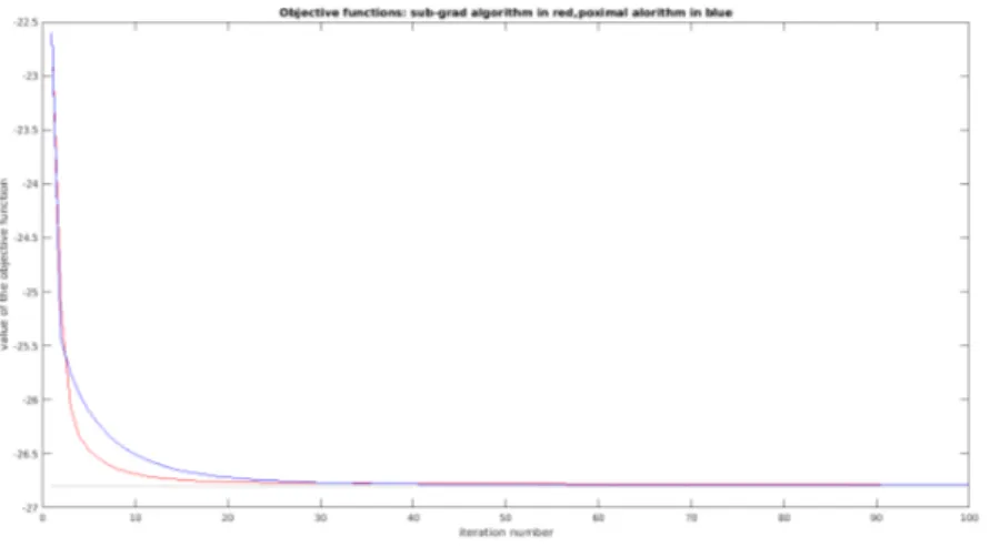
The parameter that will be used the most during this work for comparing the algorithms is the value of the objective function, in 3.4 is show an example trend of the objective function for the solution provided by both the algorithm.

(29)

3.2. Convergence

Figure 3.2: 4 bases 4 users - Trend of the solution owned by a base, dotted lines are optimal values of the single powers

Figure 3.3: Every solution concerning the mobile user 1, gathered from all the bases in a 9 bases system

(30)

Figure 3.4: Trend of the objective function - red for subgradient algorithm and blue for prox-imal minimization

(31)

3.3. Single user

3.3 Single user

In this first experiment the algorithms have been ran on a system consisting of m bases and

n = m mobile users for 100 times. Every base has only one user attached and in every instance

the bases grid has been kept the same, while the mobile users were relocated randomly. This first test has been held for highlighting the relative error achieved by the algorithm after a number of iterations. In this case the max in the objective function is obsolete, having only one agent per base.

The results are shown in the histograms,where the results are compared after different itera-tions.

4 Bases 4 Users

Figure 3.5: Map with 4 bases and 4 users, the dotted lines connect bases

In 3.6 are shown the histograms of the results with the same relative error, after different iterations.

In the case in which all the bases are paired with one mobile user only, the trend of the ob-jective function for both the algorithm is smooth,as shown in 3.7.

(32)

Figure 3.6: Blue bars for the proximal minimization and red for the sub gradient

Figure 3.7: Trend of the object function , in red the sub-gradient algorithm and in blue the proximal minimization

9 Bases 9 Users

A map extracted from a simulation is shown in 3.8.

Now that the system is bigger, an agent has to wait more than one iterations for mixing the information properly.

The results regarding this simulation are shown in 3.9.

(33)

(34)

10 Bases 10 Users

A map extracted from a simulation is shown in 3.11,it is noticeable that this time the shape is non conventional.

The results regarding this simulation are shown in 3.12.

(35)

A map extracted from a simulation is shown in 3.14,in which the bases are 5 Km far from each other.

The results regarding this simulation are shown in 3.15. Also in this case the objective func-tion is smooth for both the algorithm, 3.16.

(36)

A map extracted from a simulation is shown in 3.17.

The results regarding this simulation are shown in 3.18. Also in this case the objective func-tion is smooth for both the algorithm, 3.19.

(37)

(38)

3.4 Multi user

This simulations focused on system with more mobile users than bases, and highlights the problems occurring with such systems. At least one mobile user is attached to every base. These cases are computationally harder to solve and require more time compared to the sin-gle user’s ones.

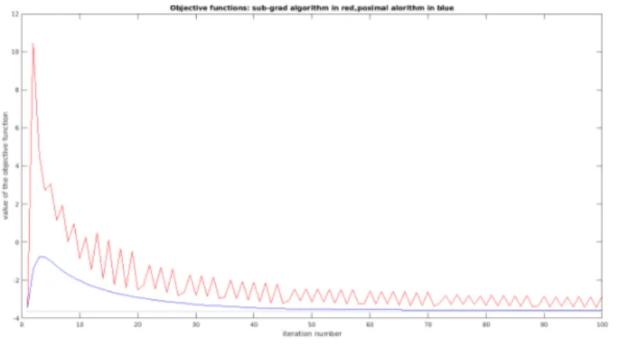
In this case the sub-gradient algorithm solutions are fluctuating, and so is the objective func-tion.

In these simulations the parameters of the system are set as in the previous simulations.

A rectangular grid of bases kept fixed and 10 users relocated at every simulation. This sim-ulation has been ran 100 times, and the results are shown in 3.21 while an example map is shown in 3.20. The objective function of a simulation are shown in 3.22.

(39)

3.4. Multi user

In this system all the bases are positioned on the same line, with the same distance between each others,in such way for maximizing the diameter of the graph. An example of the map is shown in 3.23 while an example of objective function is shown in 3.25. It is noticeable how the objective function of the sub-gradient algorithm changes values every iteration in a non-smooth way. The results regarding the relative tolerance are shown in 3.24.

The simulation has been done 100 times, with a random relocation of the mobile users at every iteration. The results are gathered in 3.24.

(40)

(41)

3.4. Multi user

Figure 3.25: Example of objective function, in red the sub-gradient one and in blue the prox-imal minimization

(42)

A rectangular grid of bases kept fixed and 10 users relocated at every simulation.

This simulation has also been ran 100 times, and the results are shown in 3.27 while an ex-ample map is shown in 3.26.

The objective function of a simulation are shown in 3.28.

(43)

3.4. Multi user

(44)

(45)

3.4. Multi user

(46)

Figure 3.34: Trend of the object function, in red the sub-gradient algorithm and in blue the proximal minimization

3.5 Step-size selection

A parameter of great importance is certainly the coefficient weighting the proximal term in the proposed distributed algorithm based on proximal minimization or, equivalently, the step-size used in the sub-gradient algorithm, which are both given by _kα_β and called "step-size" for simplicity. Its value affects every aspect of the simulation, from convergence time to tolerance.

While beta has been kept the same(β = 0.7) for all the simulations,we tried to check the in-fluence ofα on the algorithm execution and on objective function. It has been also noticed that the step-size affects the two algorithms in a different way. In these simulations the same system has been ran for every α in range 0-20, and for every configuration the system has been run for twenty times.

Singular results are shown as well as average results.

4 Bases 4 Users

In 3.35 we can see how the value of the integral of the distance between the objective function and the optimal value of the objective function varies whenα is modified. We can notice that

(47)

3.5. Step-size selection

both the algorithm have the minimum whenα is near to the number of bases,and that the proximal minimization algorithm works better whenα increases.

Figure 3.35: Red line for sub-gradient algorithm and blue for proximal minimization

Concerning the relative error of the objective function we can notice from 3.36 that the best working point is still whenα is near to the number of bases.

(48)

9 Bases 9 Users

Also in this case the behavior is similar to the previous,as shown is 3.37. The proximal mini-mization algorithm still has a better behavior , especially whenα grows up.

Concerning the relative error of the objective function we can notice from 3.38 that the best working point is still whenα is near to the number of bases.

(49)

(50)

In this case more mobile users than bases are present in the system, as it can be noticed this changes the behavior of the algorithms as seen in 3.39 and in 3.40 for the tolerance.

The proximal minimization algorithm still has a better behavior , especially whenα grows up.

(51)

Figure 3.40: Relative error after 200 iterations-Red line for sub-gradient algorithm and blue for proximal minimization

We next examine the effect of changingβ, while the α value is kept equal the the number of bases in every simulation. Also in this case we will use 2 indicators for the performance of both the algorithms, the first one is the relative error achieved after 50 iterations while the second one is the value of the area between the objective function value and the optimal value in the first 50 iterations. This second parameter tries to highlighter the overalls perfor-mance of the algorithms during the initial phase of the execution. In all the next simulations a configuration has been run 20 times, and at each time the system was solved withβ rang-ing different values. The interestrang-ing values are between 0.5 and 1, in this range the algorithms converge.

4 bases 4 users

(52)

Figure 3.41: value of the objective function area in the first 50 iterations

(53)

4 bases 10 users

In 3.43 and 3.44 are shown the results for a system with 4 bases and 10 users. The proximal minimization preserves a better performances in the case with more users.

(54)

9 bases 9 users

In 3.45 and 3.46 are shown the results for a system with 9 bases and 9 users. As it can be noticed in the graphs, when users and bases are in the same number the minimum is marked and the value of the step size assumes a more important role.

(55)

In 3.47 and 3.48 are shown the results for a system with 9 bases and 15 users.

(56)

be-Chapter 3. Numerical simulation results

tween the objective function and optimal value, which can be considered as the amount of resources wasted. We next consider jointly their effect. In this simulation the systems has been solved withβ and α ranging in a closed set of values.

4 bases 4 users

In figure 3.49 and 3.50 is shown the impact of the step size on the algorithms, while in 3.51 and 3.52 is shown the relative error.

Figure 3.49: subgradient algorithm - value of the objective function area in the first 50 itera-tions

(57)

Figure 3.51: subgradient algorithm - value of the relative error after 50 iterations

Figure 3.52: proximal algorithm - value of the relative error after 50 iterations

9 bases 9 users

(58)

Figure 3.54: proximal algorithm - value of the objective function area in the first 50 iterations

(59)

(60)

(61)

Figure 3.59: subgradient algorithm - value of the relative error after 50 iterations

Figure 3.60: proximal algorithm - value of the relative error after 50 iterations

(62)

Figure 3.62: proximal algorithm - value of the objective function area in the first 50 iterations

(63)

(64)

3.6 Execution time

This experiment has been held for highlighting the time of execution of both the algorithms. Analyzing the algorithms steps is it already possible to observe that the sub-gradient algo-rithm has an easier execution and is computationally easier to solve than the proximal mini-mization algorithm.

This is due to the fact that the sub-gradient algorithm can be run without using optimization instrument or software, but needs only a gradient to be found at every iteration. The gradi-ent analytic form can be calculated once and stored by the bases for being evaluated every iteration, making the algorithm even faster. This certainly makes the sub-gradient algorithm faster than the proxiamal in terms of iterations/time.

The results for the experiments with a mobile user per base are shown in 3.65, where we have depicted in order the systems from 4 bases and 4 users until 25 bases and 25 users. The dotted lines depict the average value for every algorithm.

(65)

3.7. Initialization influence

3.7 Initialization influence

This sections focuses on the differences that a different initialization of the algorithms may have on the results. A natural way of starting the algorithms could be that of using the local optima solution associated with the base. In a big system could be of interest to study how the algorithms proceed when the initialization is a sort of "shared optima",which consists of a common vector created by all the bases through sharing their optimal solution. This vector has in every position i the power of the mobile user suggested by the base at which the mobile user i is attached to. In this way the network has to exchange information before the algorithm start.

4x4

In this experiment a 4 bases network has been run 100 times, and every time the configura-tion was solved either both with the local optima initializaconfigura-tion and with the shared optima. For the sub-gradient algorithm results are shown in 3.67, while for the proximal one in 3.68.

(66)

Figure 3.67: Sub-gradient algorithm Red bars for local optima and blue for shared optima

Figure 3.68: Proximal algorithm Red bars for local optima and blue for shared optima

16x16

In this experiment a 16 bases network has been run 100 times, and every time the configura-tion was solved either both with the local optima initializaconfigura-tion and with the shared optima. The results are similar to the previous ones.

(67)

3.7. Initialization influence

4x8

In this experiment a 4 bases network with 8 mobile users has been run 100 times, and every time the configuration was solved either both with the local optima initialization and with the shared optima. In this case the results change,and show a different trend of the object function.

(68)

9x15

In this experiment a 9 bases network with 15 mobile users has been run 100 times, and every time the configuration was solved either both with the local optima initialization and with the shared optima. In this case the results show how this methods works better for the proximal algorithms than with the sub-gradient algorithm.

(69)

3.8. Average solution comparison

3.8 Average solution comparison

In this experiment, the real objective function value is compared to the value obtained when the average solution of all the agents is used as power vector. Reasonably it is expected that the real powers are more accurate especially in big systems, where the information takes more time to spread. This can be useful to understand which solution is better in the case the algorithm stops before the solution has spread to all the agents, in fact after a finite amount of time all the agents hold the same solution.

The comparison is shown for the same algorithm, in the cases in which the base has only one use attached and in the case with more users. The simulations have been ran 100 times for every system configuration. In 3.75 and 3.77 are gathered the results for the cases in which

(70)

there is only one user for every base, while in 3.76 and 3.78 for the case with more user for every base.

(71)

3.8. Average solution comparison

Figure 3.76: Proximal algorithm, cyan for real powers and green for average

(72)

Figure 3.78: Proximal algorithm, cyan for real powers and green for average

3.9 Single base solution comparison

Apart of optimization, these algorithm have also the purpose of spreading the solution to all the bases in the network. This solution will be the same for every base after a finite amount of iterations, but during the execution every solution differs from the others and is also likely to differ from the vector used by the mobile users.

It could be of interest to confront the solutions held by the agents with the one actually used by the mobile users during the execution of the algorithms. An example is shown in 3.79, where the power vector currently used is shown in blue while the solution held from the bases are depicted in black. It is noticeable how the singular solutions of all the bases take more time to approach the optimal solution.

(73)

3.9. Single base solution comparison

Figure 3.79: Proximal algorithm, Blue for real powers and black for agents solutions

For every simulation, the average value of the objective function given by the solutions of the agents is used to calculate the relative error with the power used by the mobile users at every iteration. The results for the simulation with a single user per base are shown in 3.80 and 3.81.

In the case in which a base might have more users than one, the relative error value is very high during the initial phase, but during the end we can notice how certain bases have a better solution than the one used by the users. This happens especially with the subgradi-ent algorithm, the results are shown in 3.82, where is shown the average value of all the 100 simulations to visualize the trend more precisely.

(74)

Figure 3.80: Relative error between single user solution and power used by users - Red for subgradient and blue for proximal algorithm

(75)

3.10. Base failure

3.10 Base failure

This last experiment focuses on the cases in which a base fails during the execution of the algorithms. As previously stated, the algorithms are capable of converging to the new optimal value also in the case of base failure, this is made possible by the way the doubly stochastic matrix is created.

Thanks to the constant upgrading of the matrix, when the neighbors of a non responsive base detect the problem, they start to upgrade the matrix until it reaches again a new doubly stochastic form.

Every simulation has been run for 100 times, in every simulation a base fails at half of the execution. It has been observed that every system moves to the new optimal solution after a base have failed, in 3.83-3.84-3.85 are shown some examples of objective function trending when a failure occurs.

It is interesting to notice how the trend of the objective function changes after the failure and become more regular and similar for both the algorithms.

(76)

Figure 3.83: 4 bases 9 users - Proximal algorithm, Blue for real powers and black for agents solutions

(77)

3.10. Base failure

(78)

(79)

4 Comparative analysis based on the

simulation results

The comparative analysis performed in this chapter is based on the simulation results of the previous chapter.

4.1 Execution speed

From the simulations is clearly visible that the sub-gradient algorithm is faster than the proxi-mal minimization in both the cases, with a single mobile user attached and also with multiple users. In our examples we observed a speed 4/5 times greater in the sub-gradient algorithm. Even if is hard to define how the complexity of the algorithms increases regarding the size, it can be observed directly on the formulations that the sub-gradient is numerically easier to solve.

This also depends on how the two algorithms are implemented, but generally in the sub-gradient one is not necessary having an optimization solver working in it, cause the Eu-clidean projection can be done with numerical comparison. If the objective function does not change, the form of its gradient remains the same for all the execution and, this allow to calculate the gradient once and store it for being used in every iteration.

Being the functions convex, a numerical solver can be efficient and fast even with great order functions,keeping the proximal algorithm efficiency high also in big systems.

It has also to be mentioned that an optimization software is more incline to fail when the system gets bigger.

(80)

Chapter 4. Comparative analysis based on the simulation results

4.2 Convergence speed in terms of iterations

One of the most important parameter with which we can compare the algorithm is how the relative error decrease with the iterations. This results are based on the relative error between the objective functions coming from the results of the algorithms and the value of the opti-mal solution. It has been noticed that the performance of the algorithms change between the case with one user for agent and the case with more.

In the simulations in which every base has only one user attached, the sub-gradient algo-rithm achieves a smaller relative error compared with the proximal minimization at the same iteration. This is true after a finite amount of iteration, in fact it has been observed that at the beginning the subgradient algorithm achieves a worse relative error than the proximal algo-rithm. This behavior seems due to the overshoot to which both the algorithms are afflicted, but has a bigger impact on the subgradient algorithm.

Regarding the case in which the mobile users are more than the bases we can notice how the proximal minimization algorithm works better in this case,the histograms show more results with less relative error for this algorithm.

It can also be noticed that the objective function relative to the sub-gradient algorithms be-comes floating when the system has more mobile users than bases. This happens because the objective function contains a max, this means that it switches at the worst connection during the optimization, trying to optimize the worst connection. This switching can be done only at the beginning of the iteration for the subgradient algorithm, while can be done also during the iteration for the proximal minimization, leading to oscillations in the first case.

This oscillation worsen the performance and can also last for for an high number of itera-tion for certain kind of configuraitera-tion. The soluitera-tion coming from the proximal minimizaitera-tion algorithm are more robust and reliable in this case.

4.3 Average solution

These two algorithms have two purposes, one is that of controlling the power of all the mo-bile users in such way to find the optimal value, while the other is to spread the solution over the bases.

When the system is run for enough time all the users end with the same solution stored,hence in this case the average solution is equal to the solution stored by every agent.