GigaFitter at CDF: Offline-Quality Track Fitting in a Nanosecond for Hadron Collider Triggers

(1)

Universit`

a di Pisa

Facolt`

a di Scienze Fisiche, Matematiche e Naturali

Tesi di Dottorato in Fisica Applicata

GigaFitter at CDF: Offline-Quality

Track Fitting in a Nanosecond for

Hadron Collider Triggers

Candidato:

Francesco Crescioli

Supervisor: Prof. Mauro Dell’Orso SSD FIS/01

(2)

(3)

(4)

(5)

List of Figures

2.1 Fermilab accelerators . . . 9

2.2 Tevatron peak luminosity and CDF Trigger upgrades 10 2.3 LHC Cross sections of various signals . . . 12

2.4 The CDF Experiment . . . 16 2.5 CDF Subdetectors . . . 16 2.6 SVX Wedges . . . 17 2.7 SVX Barrels . . . 18 2.8 Three-level Trigger at CDF . . . 19 2.9 CDF L1 Electrons . . . 21 2.10 CDF L1 Muons . . . 21

2.11 Muon trigger efficiency . . . 23

2.12 Muon trigger efficiency with tracking . . . 24

2.13 CDF online D0 mass peak . . . 25

2.14 B0 → hh . . . 26

2.15 Selections for B0 → hh analysis . . . 27

2.16 Bs oscillation in CDF and DZero . . . 28

2.17 Z → b¯b at CDF . . . 29

2.18 B-jet trigger cross section . . . 30

3.1 Unidimensional non-linear manifold in R2 1 . . . 35

(10)

4.3 SVT Dataflow and Hardware scheme . . . 47

4.4 SVT Impact parameter vs φ . . . 50

4.5 CDF beam profile: SVT and offline . . . 52

4.6 SVT impact parameter resolution . . . 52

4.7 SVT efficiency in 2003 . . . 53

4.8 D0 yield gain after 4/5 introduction . . . 55

4.9 SVT Timing tails and upgrades . . . 57

5.1 GF vs TF++ differences: χ2 . . . 64

5.2 GF vs TF++ differences: d0 . . . 65

5.3 GF vs TF++ differences: c . . . 66

5.4 GF vs TF++ differences: φ . . . 67

5.5 The Pulsar board . . . 70

5.6 The GigaFitter mezzanine . . . 70

5.7 The GigaFitter system installed . . . 72

5.8 GF Pulsar Scheme . . . 75 5.9 GF Mezzanine Scheme . . . 76 5.10 GF Fitter module . . . 77 5.11 GF Combiner module . . . 78 5.12 GF DSP Fitter unit . . . 81 5.13 GF Comparator unit . . . 82 5.14 GF Spy Buffers . . . 84

6.1 Global SVT Timing: GF and TF++ . . . 91

6.2 SVT Timing vs Number of hit combinations . . . 92

6.3 SVT Timing vs Number of fits . . . 94

6.4 SVT (GF, TF++, standard data banks) Efficiency and fake rate at high luminosity . . . 97

6.5 SVT (GF, TF++, standard data banks) Efficiency: impact parameter and pT . . . 98

6.6 SVT Efficiency vs cot(θ) with standard banks . . . . 99

6.7 SVT Efficiency vs cot(θ) comparison with new 433346 banks . . . 100

(11)

LIST OF FIGURES

6.8 SVT (GF, TF++, 544446 data banks) Efficiency and

fake rate at high luminosity . . . 101

6.9 SVT (GF, TF++, 544446 data banks) Efficiency:

im-pact parameter and pT . . . 102

6.10 SVT Efficiency vs cot(θ) comparison with new 544446

banks . . . 103

6.11 Number of combinations per road with standard banks and 544446 banks . . . 104 6.12 Maximum number of roads per wedge with standard

banks and 544446 banks . . . 107 6.13 Maximum number of roads per wedge with standard

(12)

(13)

List of Tables

5.1 HitBuffer++ to GigaFitter packet format . . . 74

5.2 GigaFitter to GhostBuster packet format . . . 74

6.1 SVT Average efficiency and fake rates with GF and

(14)

(15)

1

Overview

This thesis concerns the GigaFitter upgrade for the Silicon Vertex Trigger (SVT), the online tracking processor in the Collider Detec-tor at Fermilab (CDF) experiment.

The GigaFitter is a track fitter of new generation, designed to replace the old SVT track fitters and to enhance the tracking pro-cessor capabilities. The reduction in fitting time by two orders of magnitude will amply enable CDF to continue to take data with high trigger efficiency for the reminder of Tevatron operations.

The GigaFitter is able to perform more than one fit per nanosec-ond, with a resolution nearly as good as that achievable offline. It has been just commissioned in CDF and its computational power is available in order to provide:

1. A better SVT efficiency (i.e. larger signal yields) and more stable performances in response to the increasing instant lu-minosity, thanks to shorter execution times;

2. A better SVT acceptance, thanks to a greater capability to cover phase space regions;

(16)

to a considerable reduction in the number of boards (15 to 1) and board-to-board connections.

Better SVT efficiency The GigaFitter allows the reconstruction

of those tracks formerly discarded by the fitters because of hardware limitations. This provides SVT with increased efficiency.

In particular, slightly different but alternative hit combinations are all fit at once, with no additional latency, in order to determine the best choice; while the former processors randomly picked one combination only.

This optimization becomes substantial at the highest Tevatron col-lider instant luminosity, because of the increased combinatorial noise, effectively opposing the SVT efficiency and impact-parameter reso-lution degradations due to high detector occupancy.

Better SVT acceptance The overcoming of previous hardware

limitations allows three significant extensions of the tracking phase-space coverage, on both coordinates and momenta.

• Extending the SVT high-quality tracking to the forward-rapidity region will expand the lepton trigger coverage into that region. • Extending the SVT acceptance lower-limit on transverse mo-menta from 2 GeV/c down to 1.5 GeV/c will significantly improve the online b-tagging capability.

• Extending the SVT acceptance upper-limit on impact param-eters from 1.5 mm up to 3 mm will substantially improve the lifetime measurements.

(17)

As a final remark, the GigaFitter has been developed with a pos-sible application to the Large Hadron Collider (LHC) experiments in mind. It is an essential ingredient in developing a hardware track trigger in that environment, where the luminosity will be two orders of magnitude higher than at Fermilab.

Tracking will be essential for virtually all triggers.

Separating b quarks or τ leptons from the enormous QCD back-ground requires tracking: a secondary vertex identifying metastable b hadrons, one or three tracks in a very narrow cone from the hadronic decay of a τ .

Even the selection of high energy electrons and muons will rely much more heavily on tracking, since the calorimeter isolation is made in-effective by the energy deposition of overlapping collisions in the beam-crossing (pile-up).

The GigaFitter performances established in this thesis are requisite for LHC track triggers.

Chapter 2, Hadron Collider experiments and Trigger, high-lights the problem of online event selection at hadron collider ex-periments and its importance for the experiment physics outreach. Section 2.1 describes the multi-level trigger approach and its imple-mentation at the CDF experiment. Section 2.2 follows with exam-ples of actual track-based triggers and their impact on physics.

In chapter 3, Tracking in High Energy Physics, the central argument is the problem of reconstructing particle trajectories in a tracking detector, in particular the challenge to perform this task with trigger timing performances. In section 3.1 I explain the SVT algorithm from a theoretical point of view.

I describe in chapter 4 the Silicon Vertex Trigger actual im-plementation, the complex hardware processor for the CDF experi-ment level 2 trigger. Section 4.1 shows the design ideas and the

(18)

per-ment through a series of upgrades; the CDF upgrade program has been essential in order to allow the SVT processor to continue its online task, despite the event complexity increase due to the accel-erator performances continuously improving. It also describes the diagnostic system and debug features used during development and commissioning of the processor and its upgrades.

The object of my thesis work, the GigaFitter, is described in chapter 5 (GigaFitter). It is the latest upgrade for the SVT pro-cessor, a new generation hardware processor for the SVT track fit-ting. I have worked on every phase of this project, from the design to the commissioning, coordinating a small group of three physicists and one engineer.

Section 5.1 outlines the design features and the improvements over the previous track fitters. In the sections 5.2 and 5.3 is the Gi-gaFitter hardware structure: three powerful FPGAs on mezzanines mounted on a standard motherboard, the Pulsar, provided of other three older FPGAs. I have worked on the validation of the first prototype and all the hardware tests of the final system.

Section 5.4 shows the logical structure of the GigaFitter. The build-ing blocks are distributed over the six interconnected FPGAs usbuild-ing three different firmwares (one for the mezzanine FPGA, one for the two Pulsar FPGAs connected to the mezzanines and one for the Pul-sar FPGA connected to the output and VME backplane). I have developed all the firmware and all the tools necessary to validate and debug them.

Section 5.5 describes the careful test procedures used to validate the system from the prototype to the installation for commission-ing. I have performed, coordinating other 3 young physicists, all of these tests: the stand alone tests in Pisa and Fermilab, the instal-lation of the final system for parasitic data taking and the planning for commissioning and decommissioning of the old system. I have

(19)

also developed the software code for the GigaFitter simulation and integration with the existing SVT debug system, CDF online mon-itoring and Run Control system.

Finally chapter 6, GigaFitter performances, reports the first measurements of the performances performed with the final system in parasitic mode. In section 6.1 I show the timing measurements comparing the old system and the GigaFitter.

The GigaFitter is still underused in this initial installation. Prospects for future SVT performances, reachable only when the new proces-sor capabilities will be exploited by CDF, have been studied using the simulation.

Section 6.2 shows the results of efficiency and fake studies I per-formed with the GigaFitter simulation, exploring new tuning pos-sibilities for the system and showing how it’s possible to gain in efficiency and acceptance thanks to the GigaFitter upgrade.

In chapter 7, Conclusions, there is a brief summary of what has been shown in this thesis, the main described topics and the obtained results.

(20)

(21)

2

Hadron Collider

experiments and

Trigger

Experiments in hadron collider high energy physics have grown to be very ambitious in recent years. The upgraded Tevatron at Fer-milab and even more the upcoming Large Hadron Collider (LHC) at CERN are in an excellent position to give conclusive answers to many open questions of fundamental physics: for example the exis-tence of supersymmetric particles, of the Higgs boson and the origin of the CP asymmetry. To reach these goals the new experiments deal with very high energy collisions, very high event rates and ex-tremely precise and huge detectors.

Along with the development of new accelerators and detectors also the algorithms and processors to analyze the collected data and extract useful information need to evolve and become more power-ful. The offline problem has required the birth of huge computing centers, the development of new world-wide computer networks and

(22)

very advanced software. Web and GRID systems have been created for this challenging task. The online problem is even more complex and a particular effort must be put into it: the most interesting processes are very rare and hidden in extremely large levels of back-ground, but only a small fraction of produced events can be recorded on tape for analysis. The online selection of events to be written on tape must be very clever and powerful to fully exploit the potential of new experiments.

The complex set of systems that analyze the data coming from the detector, extracts the useful information and makes the deci-sion about whether or not to write that event on tape is called the “trigger”. A very important part of the trigger is the one that re-constructs charged particles trajectories in the tracking detector: with this knowledge it is possible to make very sophisticated and powerful selections. The information from the tracking detector is often not used at its best at trigger level because of the big amount of data to process (the tracking detector is usually the one that produces most of the data) and the difficult task of trajectory re-construction. Modern hardware along with clever algorithms allows us to fully exploit tracks in the trigger environment.

The SVT processor at CDF has been a pioneer in this field. The CDF experiment is located at the Tevatron accelerator (figure 2.1) at Fermilab (Batavia, IL, USA). The Tevatron is a proton-antiproton collider with a center of mass energy of 1.96 TeV and

reached peak luminosity up to 3.5 × 1032 cm−2s−1 as of 2009. SVT

was installed in 2000 providing for the first time at an hadron col-lider experiment offline quality tracks to the trigger decision algo-rithm.

In general dedicated hardware is considered powerful but usually difficult to upgrade and not flexible. SVT has instead proven that a

(23)

Figure 2.1: Fermilab accelerators - A simple scheme of the accelerator chain at Fermilab.

properly designed hardware can also be flexible enough to prospect upgrades to enhance further its capabilities and to cope with in-creasing detector occupancy. In 2003 when the Tevatron perfor-mances started to improve SVT showed the need of more powerful computation capabilities. No upgrade plan was in CDF. It could happen that the difficulties of an unpredicted upgrade could make void the effort of building SVT, that was quickly becoming obsolete. However the high degree of organization and standardization inside the CDF trigger and SVT system allowed a very quick upgrade, even if the function performed by SVT is very complex. SVT was upgraded into just 2 years, exploiting the experience of previous scheduled CDF upgrades: the Pulsar design (13) and the Global L2 upgrade. The Pulsar board, an FPGA based general purpose board was heavily used to implement all the SVT functions. The figure 2.2 shows the Tevatron instant luminosity grow and the correlated CDF actions to keep the trigger efficient. The SVT upgrade com-missioning took place in the summer 2005 while the experiment was taking data. A phased installation was chosen: boards were replaced

(24)

Figure 2.2: Tevatron peak luminosity and CDF Trigger upgrades - This figure shows the various upgrades programs that CDF made at the trigger system to adapt to increasing luminosity. The performance of the accelerator has steadily increased over time and it’s foreseen to be able to beat the 3.5 × 1032 cm−2s−1 record before the end of operations in 2011/2012. Many of these upgrades were unpredicted and exploited the experience and method used during the successful SVT upgrade of 2006.

(25)

2.1 Online event selection

gradually, exploiting the short time between stores1. This phased

procedure allowed for quick recovery if there were failures, since each small change was immediately checked before going ahead. The power added to the experiment without any risk for the data taking convinced the collaboration to proceed with other impor-tant unpredicted trigger hardware upgrades, to fix problems caused to the trigger by the increasing Tevatron performances (shown in figure 2.2). The very last upgrade is again for SVT and it is the GigaFitter, the object of this thesis.

The GigaFitter will allow the SVT processor to deal with the in-creased luminosity of the Tevatron collider and also gives a prospec-tive of what is possible at more challenging experiments such as at LHC.

2.1 Online event selection

Developing algorithms for online selection of events is a crucial step to fully exploit potential of new experiments.

At CDF the collision rate is about 2 MHz and at an

instanta-neous luminosity of 3 × 1032 cm−2s−1 the average number of

inter-actions per bunch crossing (pileup) is 6 (3) (396 ns bunch spacing). The rate at which events can be written on tape is about 100/s.

At the new LHC experiments the problem is even more harsh: the collision rate is 40 MHz and at an instantaneous luminosity

of 1034 cm−2s−1 there are 25 pileup interactions, while the rate at

which events can be written on tape is still about 100/s (the storage 1_{A store is the period when the Tevatron accelerator is making collisions for High Energy}

Physics experiments. Its duration depends on initial luminosity of the store and accelerator status. During the SVT upgrade was about a day with few hours between stores, now it’s typically 10-12 hours with 1-2 hours between stores.

(26)

technology is much faster at LHC but events are bigger).

The trigger system must perform a very stringent selection, re-ducing the rate of events of several orders of magnitude. This selec-tion must be as sophisticate as possible in order to suppress back-ground events while saving signal events.

Figure 2.3: LHC Cross sections of various signals - It’s shown the expected rate of events and the relative cross sections between various kind of signals and background events at the LHC baseline luminosity of 1034

cm−2s−1

(27)

2.3: the total rate of produced events at LHC baseline luminosity

is about 109 every second and only 100/s can be written on tape.

However we must be sure to write among them a possible Standard Model (SM) Higgs of 115 GeV decaying in two photons that is pro-duced roughly every hour, the even rarest SM Higgs of 180 GeV decaying in four leptons and so on. The trigger must be able to select a rich variety of interesting but extremely rare events, each one with its peculiar detector response, but be able to reject the overwhelming amount of uninteresting events.

The physics outreach of the experiment is determined by the trigger capabilities as much as by the accelerator and detector per-formances: producing an hypothetical 500 GeV SUSY Higgs every minute is useful only if the experiment is able to select and store that event with an high efficiency. If the trigger is inefficient, for example only 1% of such events are selected, the experiment is equivalent to another one that can exploit only a hundredth of the luminosity but with a better, full efficient trigger.

2.1.1 Multi-level trigger

Hadron collider experiments are made by many different subdetec-tors, the tracking detector being one of them, and each subdetector has its own data channels, it’s own time response and readout band-width. Not all subdetectors can be read at every collision. At CDF, for example, the silicon tracker can be read at a maximum rate of

30 kHz without damaging the sensors and causing deadtime1 to the

experiment.

1_{“deadtime” is the technical jargon to call the period when experiment has data, but the}

(28)

Furthermore the algorithms to extract useful information from sam-pled data have a wide range of timing and complexity: finding global calorimetric parameters (sum of all transverse energies, miss-ing transverse energy, for example) is very fast, findmiss-ing jets (clusters of energy in calorimeter) is slower like finding tracks with offline quality. Also the trigger decision algorithm, that apply cuts on the parameters reconstructed by the various trigger processors, might be of a wide range of complexity and timing.

In this context it is not convenient to use all processors at one time on the same event, because it would be always necessary to wait for the slowest, and apply an efficient but complex and slow decision. This strategy would lead to a certain amount of time where collision would happen but the system would be busy and the data would be lost.

It is much more convenient to group processors based on their band-width and latency, then organize the trigger in a pipelined multi level scheme: at the first level the fastest algorithms are executed and a first decision is taken reducing the input rate that has to be analyzed by the slower processors at level 2. At the second level the second fastest algorithms are executed on data collected by the first level and a second decision is taken and so on. This scheme allows to employ complex algorithms that otherwise would generate dead-time at later levels characterized by lower input rates. The amount of data that needs to be buffered before the final decision is also minimized.

This strategy suggests to put slower processors at high levels of the trigger, but for the sake of collecting high purity data it’s manda-tory to be able to do sophisticate selections from the first levels of trigger. The solution is to employ powerful dedicated processors in order to make complex and precise algorithms fast enough to be put in the first levels of trigger. This is the strategy that CDF has fol-lowed for triggers based on reconstructed tracks, pushing tracking

(29)

processors at the first two levels of trigger and allowing collection of high quality data.

2.1.2 Trigger at CDF

2.1.2.1 The CDF experiment

The CDF detector has the typical structure of a collider experi-ment: many sensors disposed in an “onion”-like structure starting from the interaction point as shown in figure 2.4. The inner de-tector is the tracker made by internal barrels equipped with silicon double-face microstrip sensors (it is subdivided in three subdetec-tors starting from interaction point: L00, SVX and ISL) followed by a multiwire drift chamber (COT). The tracking detector is inside a superconducting solenoid magnet. After the magnet there are the calorimeters: preshower, electromagnetic calorimeter and hadronic calorimeter. The outermost detectors are the muon detecting sys-tems. A full description is found in (4).

Figure 2.5 shows one quadrant of the longitudinal section of the CDF tracking system. The outermost detector is the Central Outer Tracker (COT) drift chamber. The COT provides full coverage for

|η| < 1, with an excellent curvature resolution of 0.15 pT(GeV)%.

The COT is the core of the integrated CDF tracking system. The COT provides 3-dimensional track reconstruction with 96 detector layers. The 96 layers are organized into 8 super-layers. Four of which are axial, while the others, called stereo, are at small angles. Inside the COT there are the silicon detectors: SVX II, ISL and L00. They are complementary to the COT. They provide an ex-cellent transverse impact parameter resolution of 27 µm.The silicon detectors provide 3-dimensional track reconstruction. The achieved longitudinal impact parameter resolution is 70 µm. Figure 2.6 shows a cross section of the SVX II. The SVX II is organized into 12 az-imuthal wedges. For each wedge there are 5 detector layers each

(30)

Figure 2.4: The CDF Experiment - An isometric drawing of the CDF experiment. Different colors highlights the various subdetector and compo-nents of the experiment. The innermost green subdetectors are the silicon microvertex detectors (ISL, SVX and L00).

Figure 2.5: CDF Subdetectors - A schematic r-z view of one half of the CDF experiment. η coverage of the various silicon tracking subsystems is highlighted.

(31)

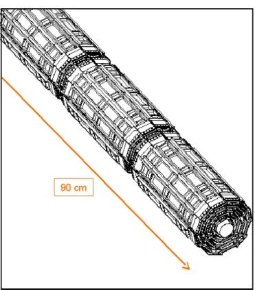
providing one axial measurement on one face of the silicon sensor and a 900 or small angle measurement on the other face. Figure 2.7 shows an isometric view of the SVX II. The SVX II is made of three mechanical barrels. Each mechanical barrel is made of two electrical barrels. In fact, within a mechanical barrel each detector element is built of two silicon sensors with independent readout paths. The two sensors are aligned longitudinally to achieve a total length of 29 cm, which is the length of each mechanical barrel. Hence, for each wedge and for each layer there are a total of 6 sensors belonging to 3 different mechanical barrels.

Figure 2.6: SVX Wedges - Each SVX barrel is made by five layers and on the r-φ plane is subdivided in 12 slices wide 30◦ φ called wedges

The L00 and ISL silicon detectors complete the silicon subsys-tems. The L00 detector, which is directly mounted on the beam pipe, provides best impact parameter resolution. The ISL detector provides up to two additional tracking layers, depending on track

(32)

Figure 2.7: SVX Barrels - SVX is made by three separate barrels (called mechanical barrels) of five layers detector in the z direction. Each barrel is made by two bonded barrels (called electrical barrels).

(33)

pseudo-rapidity, that allow standalone silicon tracking. In particu-lar, ISL allows to extend tracking beyond the COT limit (|η| < 1), and up to |η| < 2. The L00 and ISL detectors are not used by the SVT.

2.1.2.2 The CDF three-level trigger

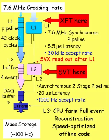
Figure 2.8: Three-level Trigger at CDF - The three levels of the CDF trigger and their bandwidth. In evidence the tracking processors: XFT (1st level) and SVT (2nd level).

In figure 2.8 is shown the three-level structure of the CDF trig-ger. The first level is a synchronous pipeline of dedicated hardware processors receiving data at the collision rate of 7.6 MHz and re-ducing the rate up to 30 kHz in 5.5 µs of latency. The second level

(34)

is asynchronous, made by dedicated processors and a final decision commercial CPU. It process the data selected by the first level and makes a decision with an average latency of 20 µs reducing the rate up to 1 kHz. There are only four event buffers at level 2 (L2), so it’s mandatory for all L2 processors to have not only the processing time with compatible average, but also short tails to avoid deadtime. The third level is a CPU farm that execute an optimized version of the offline reconstruction algorithms. The third level reduces the rate of events to 100 Hz for permanent storage.

2.2 Tracks in trigger: examples

It’s worth to notice that in CDF a tracking processor is present starting from the first level of trigger. In fact at level one there is the XFT processor (3) for reconstruction of transverse trajectories segments in the COT chamber. Moreover at the second level there is the SVT processor for offline quality reconstruction using SVX and XFT tracks. XFT is also used at level 2 for 3D confirmation of previously 2D reconstructed segments.

2.2.1 Electron and muons in CDF

In CDF the use of tracks at level 1 has been extremely important for lepton identification.

Figure 2.9 shows that 8 GeV electrons can be selected at CDF oc-cupying a very small part of the whole level 1 bandwidth (0.180 kHz of a total of 30 kHz). The rate is proportional to the instant luminosity, as happens for pure physics samples where the fakes

are negligible. CDF rates are determined by the coincidence of

(35)

2.2 Tracks in trigger: examples

only the ECAL does not distinguish between electrons and photons.

The large background of photons from the π0 decay would produce

large rates and would force the experiment to set much higher L1 thresholds. The L1 coincidence between the EM cluster and a track

segment distinguishes the electrons from the large π0 background

and reduce significantly the L1 thresholds.

Figure 2.9: CDF L1 Electrons - Level 1 rate for trigger selection of electrons with pT > 8 GeV. The occupied bandwidth is a very small fraction

(0.180 kHz) of the total available bandwidth (30 kHz).

Figure 2.10: CDF L1 Muons - Level 1 rate for trigger selection of muons with pT > 4 GeV. The occupied bandwidth is a very small fraction (0.180

(36)

Figure 2.10 shows that also soft muons (4 GeV) can be selected occupying a small trigger bandwidth. The L1 muon trigger is first of all based on the measurement in the outer muon chambers. How-ever the momentum resolution is lower compared to the capability of the tracking detector, being limited by multiple scattering, and the measurement of the impact parameter is very poor. Thus, a trigger mainly thought to select prompt muons from boson decays based only on muon chamber measurements suffers of many back-grounds: (a) promoted muons: real, low-momentum muons (mostly from b or c-decays), which are mis-measured and appear to have a

pT above threshold. (b) muons that are product decays of pions and

kaons, (c) fake muons due to noise correlated to beam not screened because the muon detector is external with respect the calorimeter. Early combination of the muon trigger chambers with precision mea-surements in the inner tracker drastically reduces the background rate.

2.2.2 High p

_T

lepton isolation in ATLAS

Another important area where track abilities should be recovered is high Pt lepton isolation. We observe in CDF the decreasing ef-ficiency of calorimeter-based isolation algorithms due to the pileup increase. The track ability to determine the high-PT primary vertex will help identify isolated electrons and muons. This would include the advantage at high luminosity of basing isolation on tracks above a PT threshold that point to the high-PT primary vertex. We have compared the calorimeter and track based isolations at LHC where the pile-up problem will be extremely more relevant.

Figure 2.11 shows that the isolation based on electromagnetic en-ergy (red points) measured at Atlas around the lepton causes strong inefficiency on the 20 GeV muon already with a little number of pile-up events. The black points show the efficiency of a selection that

(37)

does not apply any isolation criteria.

Figure 2.11: Muon trigger efficiency - The figure shows the efficiency versus the number of pile up events of two muon triggers, one with isolation (red) and one without (black), for the Atlas experiment at LHC. The trigger with isolation suffers from the increase of the number of pile-up events.

Figure 2.12 shows that applying a threshold over the Pt sum over all tracks above 1 GeV and inside a cone around the lepton (black points) produces a better result. Requiring the z0 of all tracks in the cone within 10mm of the muon track z0 (red points) produces a perfect result.

(38)

Figure 2.12: Muon trigger efficiency with tracking - The figure shows the efficiency versus the number of pile up events of two muon triggers plus isolation done with inner tracker for the Atlas experiment at LHC. The black points are a cone-based isolation, while the red points are obtained also re-quiring z0 match with muon track.

(39)

2.2.3 Two-Track Trigger

The most revolutionary use of tracks ever seen at an hadron collider, at both level 1 and level 2 is certainly the CDF Two-Track Trigger (TTT). It works on tracks above 1.5-2 GeV. Figure 2.13 shows the Two Track Trigger power.

Figure 2.13: CDF online D0 _{mass peak - Using data collected with Two}

Track Trigger (SVT) the D0 _{mass peak can be used online to monitor the}

trigger.

It shows the online invariant mass distribution of track pairs with large impact parameter. We monitor the SVT efficiency run by run

with the online reconstructed D0 signal. The 5 GeV/c2 region shows

a very low background level.

With 1 fb−1 of data CDF has reconstructed a striking B0 →

hh signal (figure 2.14) (18): an excellent example of the concrete possibility of reconstructing rare and ”background-looking” signals, when a high-performance trigger and a sophisticated offline analysis are combined.

The plot in figure 2.15 is very interesting and shows how much background would cover the Ks, D0 and B peaks if the CDF tracking detectors were not used for the trigger selection. The plot shows the

(40)

Figure 2.14: B0 _{→ hh - The figure shows the ππ invariant mass distribution}

with reconstructed B0 _{→ hh decays. Data was collected using SVT based}

(41)

background (blue, measured on data) and the B0 → hh signal (red)

cross section as a function of the applied selection criteria (17). The request of two XFT tracks at L1 and of two SVT tracks with large impact parameter at L2 reduces the level of background of several

orders of magnitude, while keeping the efficiency on the B0 → hh

signal at a few percent level. The purity of the selected sample is enormously increased. Since the B-physics has a limited rate budget, the better purity allows CDF to increase by several orders of magnitude its efficiency for the hadronic B decay modes.

Figure 2.15: Selections for B0 _{→ hh analysis - The effect of the various}

selection cuts applied for the B0 _{→ hh analysis on both signal (red) and}

background (blue).

Historically, B-physics events have been selected at hadron col-liders by triggers based on lepton identification. Trigger selections

(42)

based on the reconstruction of secondary decay vertices increase the b-quark identification efficiency and allow collecting otherwise inaccessible hadronic decay modes. The availability of the hadronic decay modes at CDF determined the different quality of the CDF and D0 (15) Bs mixing measurements (see Figure 2.16).

Figure 2.16: Bs oscillation in CDF and DZero - DZero and CDF, both

Tevatron experiments, have published an analysis on Bs oscillation. CDF

had the advantage of much more events collected by its trigger.

SVT had an extremely significant impact on the CDF physics

program. It has been essential for the Bs mixing frequency

measure-ment (1), and the first observation of the rare charmless decay modes

of the Bs (2) and Λb which complement the existing “Beauty

Fac-tories” information on Bd charmless decays (10). These extremely

challenging measurements and first observations would have been completely out of the CDF reach without the SVT. Severe con-straints on several extension of the SM already arise from the new CDF measurements and will become even more stringent when the precision of the theoretical calculations will reach the current level of experimental accuracy.

(43)

2.2.4 High p

_T

triggers in CDF

The SVT IP trigger has been used to collect a sample reach of b-jets

allowing the observation of an excess of Z → b¯b events (figure 2.17).

Figure 2.17: Z → b¯b at CDF - Preliminary analysis of Z → b¯b signal at CDF, data collected with SVT trigger.

The time made available to the final L2 CPU by the SVT up-grade allowed to reinforce the b-jet selection that initially was based, like for B-physics events, simply on the large IP requirement of one or two tracks. The b-jet trigger has been recently structured requir-ing:

• two towers with ET > 5 GeV and two XFT tracks with pT >

1.5 GeV at level1

• 2 central jets with ET > 15 GeV, 2 tracks (seen by both SVT

and XFT) matched to one jet, with Rb > 0.1 cm, d0 > 90 µm

for both tracks at level 2.

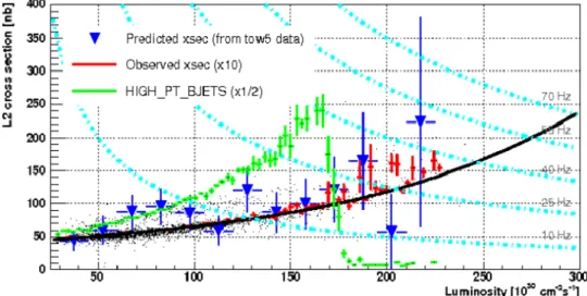
Figure 2.18 shows the trigger cross section before the improve-ment (green curve) and after (red-blue points) as a function of the instant luminosity. The green curve is stopped early because the

(44)

fakes increase too much with the detector occupancy. The new more complex algorithm increases the sample purity and allows the use of the trigger at all Tevatron instant luminosities, occupying only 70 Hz (see the light blue lines indicating the points at constant

L2 rate in the plot) at the maximum of 3 · 1032 instant luminosity.

Figure 2.18: B-jet trigger cross section - The trigger cross section for the new SVT based b-jet trigger at CDF is shown (red and blue) with respect to the old trigger (green).

(45)

3

Tracking in High

Energy Physics

Tracking algorithms reconstruct the trajectory of a charged particle going through a sub-detector of the experiment called tracker.

From the the trajectory it is possible to extract very useful in-formations for event selection. If the tracker is within a magnetic field, for example a solenoidal field oriented along the beam axis, it is possible to reconstruct the transverse momentum of the particle from the curvature of its trajectory. Reconstructing with great pre-cision the track allows the primary vertex identification and also to find secondary decay vertices and thus identify events with particles with long life (b-quark, taus), extremely useful to select physics of interest.

Charged particle tracking is a very rich source of information, in fact it’s a major technique in offline analysis where most sophisti-cated algorithms were developed.

(46)

performance suitable for trigger decision, but quality similar to of-fline tracking it’s a very challenging task. To analyze the problem we must start from how the information is recorded in the tracker sub-detector.

Usually the tracker is composed by several detecting layers with known geometry where the crossing of the charged particles is ob-served in one or two coordinates on the layer. SVX, the inner silicon tracker of CDF, it’s made of five cylinder layers of different radiuses, concentric with the beam axis. Each layer is equipped with double face microstrip detectors.

When a charged particle cross a tracking detector, for exam-ple the five-layer SVX detector, its passage is observed as five strip hits, one in each layer. The tracking algorithm must reconstruct the particle trajectory from the position of this five strips. This is not the only task of the tracking algorithm: if, for example, two particles cross the detector the signal will be ten strip hits, two in each layer, but there’s no additional information that suggests which hit was produced by which particle. The tracking algorithm must also solve the combinatorial problem associating hits to candidate tracks, selecting the ones that are real tracks and rejecting the fakes. The problem of associating hits to track candidates is as im-portant as reconstructing trajectory parameters from the candidate itself. This is a very time consuming task for the tracking algorithm, especially in modern experiments where hundreds if not thousands of charged particles are present at the same time, together with the remnant signal of the previous collisions (pile-up) and a certain amount of random noise.

(47)

3.1 The SVT Algorithm

The SVT (Silicon Vertex Trigger) algorithm was developed to re-construct the parameters curvature (c), impact parameter (d) and

azimuthal angle (φ)1 of the charged particles in the silicon detector

of CDF, SVX. SVT is designed to provide reconstructed informa-tion to the Level 2 trigger decision algorithm.

The algorithm exploits the information coming from five layers of the SVX detector (using only one face of the double face layers) plus the parameters c and φ reconstructed by the XFT processors. XFT is a tracking processor for the Level 1 trigger of CDF which recon-struct trajectories of particles crossing the multiwire drift chamber (COT) that surrounds SVX and described here (25).

The SVT algorithm is however a very general approach to the tracking problem. I will use the real SVT in CDF to describe the algorithm details, however the arguments described here are easily extended to any tracking problem.

The algorithm is subdivided in two distinct phases: the first phase finds trajectories using low spatial resolution information, as-sociating higher resolution strip hits to track candidates, the sec-ond phase does the combinatorics and finds high resolution track parameters fitting all the combinations inside each low resolution track candidate.

1_{Curvature is defined as} q

2R where q is the particle charge and R is the helix radius of the

trajectory. The impact parameter is the minimum distance of the trajectory from the z axis (oriented as the magnetic field), defined as d = |q| · (px2

0+ y20− R) where (x0, y0) is the nearest

point of the trajectory to the origin of axis on the transverse plane. The angle φ is the direction of the particle on the transverse plane in the point (x0, y0).

(48)

The association of hits to a track candidate is usually a huge combi-natorial problem, very time consuming, so an algorithm that want to solve it in time for trigger decision must find a clever and effective solution.

We start to look at this problem: how the combinations of hits coming from real charged particles differ with respect to the generic random combination?

If we look at the n-tuple of hits as a point in a n-dimensional space, where n is the number of detecting layers, and we eliminate every possible error of measurement or statistical physical effect we’ll see that the points in n-dimension that are coming from real particles belong to a well defined m-dimensional manifold where m is the number of free parameters in the trajectory equation.

This means we can write n − m equations of the hit coordinates ~

x, called constraint equations:

fi(~x) = 0

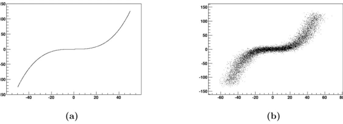
For example in SVT at CDF we have a 6 dimensional space (4 coordinates from SVX, 2 from XFT) while the trajectory equation being constrained in the transverse plane has 3 free parameters (c, d, φ). The resulting manifold is 3-dimensional and we have three constraint equations. The simpler case of a unidimensional

mani-fold in R2 easy to be represented as a plot is shown in figure 3.1 (a)

as a graphical example.

The trajectory parameters can also be a set of local coordinates on the manifold. We have to find a general method to identify n-tuples of coordinates produced by from real particles - they satisfy

(49)

(a) (b)

Figure 3.1: Unidimensional non-linear manifold in R2: (a) without mea-surement errors and (b) with Gaussian noise on the two coordinates.

fi(~x) = 0 - and a method to find track parameters - measuring the

position of the n-tuple in the local coordinates of the manifold. Up to now measurement errors or other physical effects of statis-tical nature like Bremsstrahlung, multiple scattering or delta rays were disregarded. If such effects are taken into account we’ll have not a simple m-dimensional manifold but a probability volume around it. An example is shown in 3.1 (b).

Computing the covariance matrix Fij of fi is a way to quantify

the characteristics of this volume. At first order is: Fij ' ∂fi ∂xk ∂fj ∂xl Mkl

Where Mkl is the covariance matrix of ~x.

With Fij it’s possible to build a χ2 function:

χ2 = X

ij

(50)

tions efi such as: e fi = Sijfj σi Sij is found diagonalizing F_ij−1: F_kl−1 = Sik δij σi Sil

From which we can rewrite the above in a more compact form:

χ2 = X

i

e fi 2

The χ2 function is used as a quality function: a decision based

on its value discriminates with the desired efficiency between ~x that

corresponds to a real trajectory and the ones who doesn’t.

In general it’s not easy to compute the efi and the charts for

the fit, but we can exploit the fact that a differentiable manifold admit locally to define a tangent hyperplane and thus linearize the problem. We can find a series of n-dimensional hypercubes where apply the linear approximation and obtain an atlas of linear charts for all the manifold. In CDF we’ll see that the geometry of the detector itself suggests how to find those regions. In figure 3.2 (a) is shown the procedure on the unidimensional manifold of figure 3.1. This way we’ll find for each one of those regions a set of constants ~vi, ci, ~wi and qj such as the constraint equations became:

˜

fi(~x) = ~vi·~x + ci

(51)

(a) (b)

Figure 3.2: Unidimensional non-linear manifold in R2: (a) areas where linear approximation is reasonable are defined and (b) principal axis are found using PCA. The parameter of interest is measured on the principal axis, while the orthogonal axis measure the probability that the point belong to the manifold.

From the knowledge of the equation of motion of the charged particle, of the detector geometry and of the statistical effects on measurements it is possible to find analytically an expression for such constants, but it’s more practical to use the principal compo-nent analysis on a data sample (simulated or real) and find directly the constants.

The principal component analysis (PCA) is a linear transforma-tion of the variables that define a new set of coordinates such as on the new first axis will lie the coordinate with the majority of vari-ance, on the second axis the coordinate with the second majority of variance and so on. The application on the example of figure 3.1 is shown in 3.2 (b).

This transformation is found computing eigenvectors and

eigen-values of the covariance matrix M of the data sample ~x: the

eigen-values quantify the variance of each axis found by the corresponding eigenvector.

(52)

It’s possible to demonstrate that the variance in a generic linear function f (~x) = ~x · ~v + c at the first order is:

σ ' ~v · M · ~v

In the ideal case without measurement errors a basis of the kernel

of matrix M define the ~vi of constraint equations efi. In the real

case the n − m eigenvectors corresponding to the n − m smallest eigenvalues will define the basis of the “kernel”, normalized such as v_i2 = _σ1

i in order to verify the definition of efi. The ci are easily found imposing D e fi E = 0: ci = P ~vi · ~x N

It’s worth to notice that this method is based only on analysis of a data sample of the response of the detector to a single charged particle: it’s possible to use real data and all the necessary informa-tion on detector geometry is automatically inserted in the constants of the constraint equations without need explicitly describe it and apply alignment corrections.

To find the constants ~wj and qj of parameters equation pi(~x) we

need again to use the matrix M coming from the data sample, but we also need to know the real parameters of the particle trajectory

˜

pi. It’s then mandatory to use a Montecarlo sample or to fit the

trajectory parameters on the real data by other means.

Minimizing the variance σ2(p − p) we find that ~_e wj and qj are:

~

wj = M−1 · ~γj

(53)

(a) (b)

Figure 3.3: Unidimensional non-linear manifold in R2: (a) coordinate axis are segmented and (b) a certain number of patters covering the manifold are found (in green).

Where ~γj = h ˜pj~xi − h ˜pji h~xi.

This method is described in detail in (24).

3.1.2 Pattern and associative memory

In 3.1.1 we have seen that the space has been subdivided in hyper-cubes covering the manifold to apply the linear approximation and to calculate the track parameters and the fit quality. This subdi-vision suggests us also a mean to solve the combinatorial problems on real events.

The hypercubes in the manifold identify the combinations that may be a particle trajectory. So it’s convenient to find a way to evaluate only those points in the hypercubes and discard the others. We define the concept of pattern: we segment the coordinate axis in a certain number of steps (in the real case of SVT the mi-crostrip of each detector layer are grouped in superstrip) and we call pattern a n-tuple of segments, one for each coordinate. The

(54)

Instead of computing the combinations of full resolution hits on each coordinate we’ll restrict the combinations only to the segments on layers. This way we’ll reduce greatly the number of combinations to try. In the current SVT each superstrip contains at maximum two non adjacent strips, so at maximum two hits, and the mean multiplicity of hits inside a superstrip is 1.2: the number of combi-nations is much less than combining all the hits in the detector.

If we have a collection of patterns (pattern bank) that cover at best the volume of all possible trajectories the tracking problem is to find which patterns are present in a given event, compute the combinations inside each pattern and perform the fit. In figure 3.3 is shown how the concept of pattern apply to the previous example of unidimensional manifold (figure 3.1).

How to perform the fit and compute parameters and fit quality for a given combination has been described, the remaining problem is how to compare a large number of patterns to the event. To solve this problem we use an associative memory.

A common random access memory, a RAM, when an address is supplied returns the data corresponding to the address. An associa-tive memory (in the computer science language is more often used the term content addressable memory or CAM) instead receives the content, look up if it’s present inside and returns eventually the ad-dress of the location where it is. Typical applications of associative memories outside of high energy physics are CPU caches or routing tables in switch and routers.

A kind of associative memory, able to receive the flux of hits coming from the detector and find all patterns for a given event,

(55)

has been completely developed by the CDF collaboration for SVT (16).

How an associative memory works can be explained with the fol-lowing example: each element of the associative memory is a pattern and is like a bingo player with his own scorecard, incoming data flux is distributed to each pattern like the numbers in bingo are read out loud. At each given number each player checks if it’s present in his own scorecard and when it makes bingo - when all superstrip in the pattern are present in the hits of a given event - it announces the win. All winning players, all pattern addresses, are collected and sent in output.

An important characteristic of the pattern bank is how well it cover the volume of all possible trajectories. As it’s usually com-puted from a finite data sample (real or Montecarlo) and the number of storable patterns is finite as well, it’s not always 100% of the vol-ume.

We define the coverage of the bank as the ratio of covered tra-jectories with respect to all possible ones. Given a fixed amount of storable pattern the biggest the volume of the pattern - in terms of the step size of the segmentation of each coordinate - the highest the coverage, but also the number of combinations of fits belonging to the pattern will be higher.

Optimization of the bank coverage is a difficult problem, the so-lution is strongly dependent from the detector characteristics. It’s anyhow true that regardless of the kind of optimization the largest the bank the highest the coverage and so the efficiency of the track-ing algorithm. In fact durtrack-ing the evolution of the associative mem-ory technology ((8, 19)) a great effort was put into pushing the density of the chips and the degree of parallelization in order to

(56)

latency. With this enhanced technology is possible also to think at applications for level 1 tracking (11, 20, 21).

(57)

4

Silicon Vertex Trigger

Figure 4.1: SVT Scheme - Input and major algorithm steps are drawn in this schematic view: input data come from SVX and XFT, SVX hits are clusterized, patterns are found in the associative memory and tracks are fitted with the high quality linear fit. The found tracks are sent to L2.

(58)

pro-scribed in detail in 3.1.

It receives SVX hits and XFT tracks for every event accepted by the level 1 trigger, performs the track reconstruction algorithm and sends the output tracks to level 2 decision processor in an average time of 20 µs (figure 4.1).

The system is made by over a hundred of 9U VME cards organized in ten 21-card crates (figure 4.2). The key elements used in building SVT were: (a) extensive use of FPGA, (b) flexible common moth-erboard for most of the functions, (c) common cabling and data format for all the cards and (d) for the most intensive computa-tional part of the algorithm (the pattern recognition in associative memory) a custom ASIC chip was developed. Another key element of design is the parallelization of all tasks and the highly symmetric structure of the whole processor.

4.1 Design and performances

The algorithm performs the following steps:

• SVX hits and XFT tracks (c and phi parameters) are received. Both are treated the same way so I’ll call them generically hits. • For each hit the corresponding superstrip is computed, and

hits are stored in a smart database ordered by superstrip • Superstrip are sent to the associative memory bank

• Patterns found in the event (roads) are received from the asso-ciative memory and patterns containing the same information (hits) are deleted (“ghost roads” removal)

(59)

4.1 Design and performances

Figure 4.2: The SVT racks - SVT is made by 104 9U VME boards in ten crates. The picture shows the four main racks containing all the system up to the Track Fitting and Final Merge and Corrections that are in other two crates in another rack.

(60)

• For each combination of hits inside each road the track fit is performed (full resolution tracks)

• All fits that under a certain χ2 _{value are collected, duplicated}

tracks characterized by different silicon hits associated with the same XFT track are deleted (“ghost tracks” removal) • Beam position is subtracted from impact parameter of each

track and a second order correction is applied on φ parameter • Finally the tracks are sent to the output

Each of these steps is handled by one or more cards that will be described in 4.1.1.

An important feature of SVT is that all of those steps, except the duplicate tracks removal and final corrections, can be executed independently in parallel on subregions of the detector. Since the

SVX detector is subdivided in twelve 30◦ φ sectors called wedges

(figure 2.6), 12 dedicated SVT pipelined processors process in par-allel data for each wedge up to the last steps.

This makes SVT a highly segmented system. This was a crucial feature during the upgrade program: the new hardware was tested on a single wedge in parasitic mode and once stable was ready for all wedges. This configuration also helps with the maintenance of the system.

4.1.1 Hardware structure

The SVT hardware is made by several different VME boards each one handling a different step of the algorithm described in 4.1. The

(61)

Figure 4.3: SVT Dataflow and Hardware scheme - The dataflow in one SVT wedge is shown up to the final stage of the Ghost Buster were all wedges are merged in a single data cable. The position of the GigaFitter in parasitic mode is highlighted.

(62)

figure 4.3, the hardware is the actual one after the 2006 upgrade. A uniform communication protocol is used for all data transfers throughout the SVT system. Data flow through unidirectional links connecting one source to one destination. The protocol is a simple pipeline transfer driven by an asynchronous Data Strobe (DS in the following text, it is an active-low signal). To maximize speed, no handshake is implemented on a word by word basis. An Hold signal is used instead as a loose handshake to prevent loss of data when the destination is busy (it is an active-low signal and will be called HOLD in the following text). Data words are sent on the cable by the source and are strobed in the destination at every positive going DS edge. The DS is driven asynchronously by the source. Correct DS timing must be guaranteed by the source. Input data are pushed into a FIFO buffer. The FIFO provides an Almost Full signal that is sent back to the source on the HOLD line. The source responds to the HOLD signal by suspending the data flow. Using Almost Full instead of Full gives the source plenty of time to stop. The source is not required to wait for an acknowledge from the des-tination device before sending the following data word, allowing the maximum data transfer rate compatible with the cable bandwidth even when transit times are long. Signals are sent over flat cable as differential TTL. The maximum DS frequency is roughly 40 MHz.

On each cable there are 21 data bits, End Packet (EP ), End Event (EE ), DS and HOLD . Data are sent as packets of words, the EP bit marks the last word of each packet: the End Packet word. The EE bit is used to mark the end of the data stream for the current event. End Event words are one-word packets so EP is also 1, the data field is used for Event Tag (8 bit), Parity (1 bit, computed on all data words of the event) and Error Flags (12 bits).

(63)

A first important VME board to describe is the Merger: it has four input and two outputs. The purpose of the board is to merge the data coming from the four inputs or any subset of them into one output. The two outputs of the board are identical copies of the merged data, but with separate hold signal handling: it has the possibility to consider or ignore one or both holds on the two out-puts. This board is used inside the SVT pipeline at various stages, but it’s also extremely useful for planning the upgrade tests and commissioning because the two outputs provide easily a copy of the data made at any stage of the SVT pipeline to a new processor to be tested.

A similar board with only the output copy feature is the Splitter: it has two inputs and four outputs. Each input is copied into two outputs with separate handling of hold signals like the Merger. This board is not used in the normal SVT pipeline but it’s used for the parasitic configuration in the GigaFitter upgrade (see 5.5).

The SVX hits coming from each wedge of each mechanical bar-rel (figure 2.7) of SVX are received by the Hit Finder (HF) boards from fiber optic links connected to the SVX readout hardware. For each wedge processor the data from three Hit Finder, one for each mechanical barrel, is merged in a Merger board along with the XFT tracks for that wedge.

Merged SVX hits and XFT tracks are sent to both the Associa-tive Memory Sequencer Road Warrior (AMSRW) board and the Hit Buffer (HB++) board. The AMSRW provides the superstrips out of the hits and sends them to the Associative Memory (AM++) boards. The AM++ boards send back to the AMSRW the roads found and the AMSRW, after a duplicate road elimination (Road Warrior function), sends them to the HB++.

The HB++ associates the received SVX and XFT information to each road found by the associative memory and sends this informa-tion to the Track Fitter (TF++) board. The TF++ computes all

(64)

tracks from all 12 wedges satisfying a certain quality cut are merged (using 4 Merger boards) and sent to the Ghost Buster (GB) board. The GB performs the duplicate tracks suppression: SVT tracks that share the same XFT segment are considered redundant and only the

one with the best χ2 is chosen, the other are suppressed.

Figure 4.4: SVT Impact parameter vs φ - The sinusoidal shape of the impact parameter vs φ plot is given by the beam position relative to the center of axis. From this plot is computed online the position and the impact parameter is corrected in the GB with this information.

The SVT is supposed to work with the beam in his nominal po-sition, for example parallel to the z-axis and with x = y = 0. In practice some misalignments and time variation of the beam posi-tion are possible thus correcposi-tions are needed. The beam posiposi-tion in the transverse plane can be calculated from the correlation be-tween impact parameter (d) and φ angle shown in figure 4.4. If the

(65)

beam position in the transverse plane is (x0, y0) the relationship

be-tween d and φ for primary vertex tracks is d = −x0sin φ + y0cos φ.

The impact parameter with respect to the position of the beam is d0 = d + x0sin φ − y0cos φ.

A beam-finding program monitors the tracks in input to the GB, fitting and reporting to the accelerator control network an updated Tevatron beamline fit every 30 seconds. The beam fit is also writ-ten to the DAQ event record and used by the GB board to correct in-situ every SVT track’s impact parameter for the sinusoidal bias vs φ resulting from the beamline’s offset from the detector origin, so that the trigger is immune to modest beam offsets. The GB also applies a tabulated second order correction to the φ parameter. The GB then sends the SVT tracks to the Level 2 processor for trigger decision.

4.1.2 Tracking resolution

The most striking SVT performance is the impact parameter resolu-tion. Figure 4.5 taken from the SVT TDR shows the comparison of SVT simulation on real RUN 1 data with the offline reconstruction. Figure 4.6 shows the real SVT resolution measured on CDF RUN II data. The expectations declared in the TDR were confirmed by the real SVT.

4.1.3 Efficiency

The tracking efficiency (very sensitive to many factors in the ex-periment), needed adjustments causing variations during time, es-pecially at the beginning of the data taking. Data taken by CDF

(66)

Figure 4.5: CDF beam profile: SVT and offline - The beam profile reconstructed with SVT tracks (red) and offline tracks (blue).

Figure 4.6: SVT impact parameter resolution - SVT resolution on impact parameter.

(67)

before June 2003 used only four silicon layers connected to the XFT segment for the pattern recognition, and requiring all of them to be fired (4/4). An important efficiency gain has been obtained imple-menting the use of the “majority logic” in the track match criteria. In fact SVT can require 4 fired layers among a total of 5 silicon layers (4/5). The gain is a “varying” number since it is a function of the detector status which, especially at the beginning, changed, even on short timescales.

Figure 4.7: SVT efficiency in 2003 - At the beginning of 2003 the SVT efficiency was limited from the status of SVX layers. The implementation of majority logic helped to overcome the non uniformity of SVX efficiency on all layers.

Figure 4.7 shows the SVT track efficiency as a function of day in 2003, when the majority was implemented. The plot shows a long data taking period, where the 0 corresponds to the first of January 2003. The track efficiency has a slow increment from 60% to 70% due to the SVX detector improvement (larger number of active strips/ladders). This 70% efficiency is the product of different concurrent contributions:

1. the single hit efficiency (95%) contributes as 954 = 81% to the

(68)

3. the χ2 cut efficiency after the track fitting (95%)

4. a geometrical acceptance due to the SVX ladder status (95%). This is the relevant part to explain the improvement from 60% to 70%

The 4/5 has been implemented in June 2003 and is shown in the plot as an additional track efficiency improvement up to 80%. Statistical errors are much larger in the last period since the track efficiency is calculated using a low-statistic sample. In fact the track

pT acceptance threshold has been increased in that period from 1.5

GeV to 2.0 GeV in order to reduce the L2 processing time, that increased a lot when the majority was implemented. Moreover, for the same goal, most of the events not used for the impact parameter selection have been forbidden to transit through SVT. Only few of them are allowed just to calculate the efficiency shown in figure 4.7. Any increment on track efficiency has an amplified effect as incre-ment on signal yields, since the searched particles are reconstructed combining multiple tracks, so the signal efficiency should be roughly a power law of the track efficiency. A simple example is shown in

figure 4.8 where the yield of the D0 is reported in the two cases of

majority activated (4/5) or turned off (4/4). An increment of 10% in track efficiency corresponds to an increment of 30% on the size

of the collected D0 sample. An even larger effect is expected on

samples that use more than 2 tracks to select the sample.

SVT, since the moment the majority was implemented, had im-pact on the level 2 dead time, because the processing time increased a lot causing large tails in the timing distribution. This effect, com-bined with a small number of level 2 buffers, caused dead time to the experiment. To reduce the dead time, the level 1 rate in input

(69)

Figure 4.8: D0 _{yield gain after 4/5 introduction - the number of D}0

(70)

tiality.

In 2003 the bandwidth was limited below 20 kHz, but it was clear that the Tevatron increasing instant luminosity would have reduced constantly the available bandwidth arriving to values below 10 kHz. The SVT upgrade solved the problem: the average SVT processing time was deacreased, but even more so the size of the tails, bringing back to CDF the full 30 kHz level1 bandwidth.

The effect of the upgrade can reliably be estimated by comparing SVT processing time before and after the upgrade at the same lu-minosity, with the same trigger path mixture. Figure 4.9 shows the improvement on the fraction of events with processing time above 50 µs as a function of luminosity, for different stages of the SVT up-grade. This fraction of events is interesting because over-threshold events directly contribute to trigger dead time.

The first improvement, installing the AMS/RW boards, reduced processing time by reducing the number of track fit candidates and reducing the pattern recognition time. The second upgrade, in-stalling the upgraded Track Fitter (TF++) board, significantly re-duces the fraction of over-threshold events by speeding up the track fitting process with faster clocks and a six-fold increase in the num-ber of fitting engines on the new board. Next, the use of 128K pat-terns reduces the number of fit combinations per recognized pattern. The upgraded Hit Buffer (HB++) further increased the processing speed by virtue of the faster clock speed on the upgraded board. Finally, the full power of the upgrade is visible after enabling all 512K patterns. The fraction of events over threshold is well below 5% at the highest luminosities available for these tests. Data tak-ing without an upgraded SVT system at these luminosities would clearly suffer huge rate penalties, as the corresponding fraction of events over threshold is roughly 25% at half the maximum tested luminosity, with a steeply rising tendency. The SVT upgrade has

(71)

Figure 4.9: SVT Timing tails and upgrades - The phased installation of new SVT hardware allowed to contain the tails of the SVT processing time along with the Tevatron peak luminosity increase.