A prediction of bone remodeling thanks to a mechanical signal on cells - Predizione del rimodellamento osseo a partire da un segnale meccanico sulle cellule

ALMA MATER STUDIORUM DI

BOLOGNA-SECONDA FACOLTÀ DI INGEGNERIA CON

SEDE A CESENA

A prediction of bone remodeling

thanks to a mechanical signal on

cells

Predizione del rimodellamento osseo a partire da un

segnale meccanico sulle cellule

Relatore: Candidato:

Luca Cristofolini Valeria Serchi

Correlatore:

Jean-Marie Crolet

(ISIFC Université de France-Comté)

SESSIONE DI LAUREA II

ANNO ACCADEMICO 2011-2012

iii

Index

2.Research background about bone remodeling……….……….13

3.The mechanical model ………..15

3.1 Longitudinal compression with vertical fibers: departing point ………17

3.1.1 Study at the macroscopic domain………..……...…….23

3.1.2 Study at the microscopic domain………...35

3.1.3 Study at the nanoscopic domain……….………47

3.1.4 Study of the piezo-electro effect …….……….…..61

3.2 Transversal compression with vertical fiber: start of the model development……… ……….63

3.2.1 Changes………..……….…..….…63

3.2.2 Study of the piezo-electro effect …….……….…..69

3.2.2 Comparison between longitudinal and transversal compression ………..………...…...69

3.3 Flexion ... 71

3.3.1 Potential difference coming from the nanoscopic domain in a flexion stress analysis……….………...…..75 3.4 Others architectures .. ………77 4. Matlab-Comsol implementation ... 93 5. Results ... 97 6. Conclusion ... 99 8.Future developments ... 101 Acknowledgements ... 103 Annex A ... 105 Annex B ... 115 Annex C ... 125

5

A prediction of bone remodeling

thanks to a mechanical signal on

cells

Abstract (English)

This text wants to explore the process of bone remodeling. The idea supported is that the signal, the cells acquire and which suggest them to change in their architectural conformation, is the potential difference on the free boundaries surfaces of collagen fibers. These ones represent the bone in the nanoscale.

This work has as subject a multiscale model. Lots of studies have been made to try to discover the relationship between a macroscopic external bone load and the cellular scale. The tree first simulations have been a longitudinal, a flexion and a transversal compression force on a full longitudinal fiber 0-0 sample.

The results showed first the great difference between a fully longitudinal stress and a flexion stress. Secondly a decrease in the potential difference has been observed in the transversal force configuration, suggesting that such a signal could be taken as the one, who leads the bone remodeling. To also exclude that the obtained results was not to attribute to a piezoelectric collagen effect and not to a mechanical load, different coupling analyses have been developed. Such analyses show this effect is really less important than the one the mechanical load is responsible of. At this point the work had to explore how bone remodeling could develop. The analyses involved different geometry and fibers percentage. Moreover at the beginning the model was to manually implement. The author, after an initial improvement of it, provided to implement a standalone version thanks to integration between Comsol Multiphysic, Matlab and Excel.

Abstract (Italiano)

Il testo vuole esplorare il processo del rimodellamento osseo.

lavoro è che il segnale, che le cellule acquisiscono e che suggerirebbe loro di cambiare la propria architettura, sia una differenza di potenziale ai capi delle fibre di collagene. Tali fibre costituiscono la struttura ossea da un punto di vista nanoscopico.

Questo lavoro ha come oggetto un modello multiscala. Molti studi sono stati fatti alfine di comprendere il legame fra un carico osseo macroscopico esterno e la scala cellulare. Le prime tre simulazioni svolte sono state una compressione longitudinale, una flessione ed una compressione trasversale di un campione composto unicamente da fibre verticali di tipo 0-0.

Per prima cosa i risultati mostravano una netta differenza fra una configurazione in completa compressione longitudinale ed una in flessione. Secondariamente, è stato osservato un decremento delle differenza di potenziale nella configurazione a compressione trasversa, suggerendo così che tale segnale sia proprio quello che guida il

6

rimodellamento. Per escludere, che il risultato di differenza di potenziale ottenuto fosse dovuto univocamente alle proprietà piezoelettriche delle fibre di collagene, e non al carico meccanico, sono state svolte analisi con accoppiamenti differenti. Un’analisi del genere ha effettivamente rivelato come questo contributo sia trascurabile rispetto alla differenza di potenziale, di cui il cui carico meccanico è responsabile. A questo punto il lavoro è consistito nell’esplorazione degli step del rimodellamento. L’analisi ha previsto sia lo studio di differenti geometrie sia di diverse percentuali fibrose. Inoltre, inizialmente, il modello era da implementare completamente manualmente. L’autore, dopo un suo iniziale sviluppo, ha implementato una versione stand-alone grazie all’interfaccia di Comsol Multiphysic, Matlab ed Excel.

7

Introduction

The goal of this text is to investigate the relationship between a macroscopic load applied on a bone sample and the signal received by the cells in the nanoscopic domain, which leads the phenomenon of bone remodeling. Collagen has, in fact, the particular characteristic of piezoelectricity. Since other studies such a signal, which pushes cells to change in their architecture, is the potential difference on the free boundaries surfaces of collagen fibers. This one would be simply called PD in the entire text. If a collagen fiber is deformed by a force, it develops a potential difference. Such a signal may be the one, which leads bone remodeling.

From a changing in PD, cells may understand that the existing configuration is not agreed with the external solicitation force. They are supposed to change in their architecture. This work is composed of several analysis steps. A mechanical model has been developed with the goal to investigate such an assumption. Lots of numeric studies have been performed to understand this phenomenon.

9

1. Bone Anatomy

Human body has his stability thanks to the skeleton. Without this one any movement would be possible, because muscles would have nothing to apply their driving force. Bone is a living tissue, which has a great complex structure. It is the connective tissue, which composes the skeleton. This one gives both support and protection to the body. A second important bone function is to store minerals. In particularly it stores Ca++, which is required to maintain a mineral homeostasis by the exchange of several ions, such as H+ and HPO4

+

.

Surly, bone is not like any other connective tissue, because his way to grow is different. In fact, while the other kinds of connective tissues grow interstitially, it grows on by addition of tissue on a cell-laden surface [8].

Several kinds of bones could be distinguished: longs, shorts and plates bones. They have different functions, depending on the place they are, and they work all together to allow body movement.

The most interesting thing is that bone tissue shows lot of structural levels. There exists a hierarchical scale, which is showed in figure 1. If this special tissue is charged with an external load, it grows up following the driving direction of the applied force.

There are a lot of hypothesis about bone remodeling. Any unified idea has been reached yet. Certainly bone is composed by subunits, which work in synergy.

As shown by the picture, several structural levels can be distinguished. In the macroscopic scale there is the bone, which has a cortical and a cancellous part. They differentiate themself for the percentage of marrow and soft tissue they contain.

Cortical bone represents the 80% of human skeletal. In long bones a soft tissue part

10

surrounded by a cortical one can been observed. The middle bone part usually is tubular and is called diaphysis. The part at the ends is bigger and is always constituted by soft tissue surrounded by cortical bone.

Simplifying, only cortical bone will be considered. In fact, considering also the soft part, would lead to an excessive difficulty for this contest. Going until the microscopic scale, structures, which have a dimension between 10 and 500 mm, as the Haversian system, the osteons and trabeculae can be founded.

In sub-microscopic domain there are the lamellae (3-7 µm) [4]. They are put all together side by side to form a lamellar structure. They are differently distributed to look like a piece of wood.

The space between them is filled with an amorfe substance rich in mucopolisaccarides (GAG). Inside this material there are lots of calcium salts, which precipitate in hydroxyapatite [3].

The nanoscopic scale includes collagen fibers, which are around 0, 5 µm, and minerals (from 100 nm to 1 mm). Finally there exists the sub-nanoscopic domain with his molecular structures under hundreds nanometers [2, 4].

Depending on the orientation of the collagen fibers, various kinds of osteons can be distinguished. The orientation is defined by the generating line.

1. 0-0: the osteon has all the lamellae composed by vertical fibers.

2. 0-90: the osteon has a lamella composed by vertical fibers and the following by concentric horizontal ones.

3. O: in the osteon there are two regions, an internal and an external one. This one is composed by only vertical fibers. The other one is composed by concentric horizontal fibers.

4. 90-90: the osteon has all the lamellae composed by concentric horizontal fibers.

The chosen names for each fibers derive from the convention of the SiNuPrOs

simulation program developed by mister Crolet and his team. The author has had to

take bone physical data from such an instrument and took care the same way of

calling different physiological parts [13, 14]. SiNuPrOs description will be exposed

in the following chapters.

By saying “bone is a living tissue”, the text indicates the presence of certain cellular types, which have the function to build and to destroy the structure in a continuous way.

11

There are three principal kinds of cells: osteoblasts, osteocytes and osteoclasts.

The first ones deal to form tissue, the seconds ones are probably osteoblasts trapped in the structure. Osteocytes are concerned with tissue maintenance and repair. Finally osteoclasts remove old tissue or damaged material [3].

The kind of cells described, work always according to a policy of energy saving. If bone is not solicited, it would be destroyed to use the energy, which is necessary to his maintain, for other corporal functions.

Even if bone remodeling phenomenon is not completely clear, sure it is at the base of bone fragility after a forced rest period.

Figure 2: picture representing the remodeling process step by step in a simplified scheme [2]

13

2. Research background about bone remodeling

The question the text wants to investigate about, and which lot of people have already tried to analyze, is which the force responsible of tissue remodeling is. In others words which signal represents the input, which pushes the cellular population to change in their architecture. From the “Integrin’s Theory” cells may have such sensors, which allow them to feel the change of external conditions. The term “integrins” indicates particular canal receptors. They allow the communication between the extracellular medium and the cells [10].

A relevant question is which is the signal, which cells feel thanks to the integrins. Several theories about that have been done. For example:

 Streaming potential: the extracellular fluid is forced to flow in the caniculae by a matrix deformation (Haversian and Volkmann). This causes ions charge induced on the surface. The osteocytes mediate this phenomenon.

 Mechanical solicitation of the osteocytes: the extracellular fluid is forced to flow in the caniculae by a matrix deformation. This flux mechanically stimulates the osteocytes.

 Damage accumulation: a bone, which is damaged for a fatigue stress, gets cracks. These ones usually end in cavities, where tension grows up relevantly. Osteocytes, which are in cavities, are greatly mechanically solicited.

 Collagen piezoelectricity: collagen is a piezoelectric material. If charged, a potential difference is generated. Such a PD is sensed by osteocytes [3].

The theory the text supports to implement a mechanical bone remodeling model is the last one: collagen piezoelectricity.

How and the way usually bone breaks and his mechanical properties are also important. Both cortical and cancellous bones would be described in these terms, even if the object of the study would be only the cortical one.

Bone is anisotropic. This characteristic is at the base of his great complexity. His form and his behavior are greatly connected to the applied loads. Since the viscous-elasticity is usually not relevant, bone is described as an elastic-linear material. Long bones are the ones, which are regularly charged by axial and bending loads. Flexion usually causes tensions bigger than these caused by axial stress. Usually cortical bone is brittle. That means that such bone part easily arrives to a break point instead of a yield point. Cortical bone breaks in preference under a traction force, because the anisotropy in less evident in compression. In traction the cemented lines open themselves and cause the break. Finally, cortical bone in long bones usually yields for normal stress rather than a tangential one. The other kinds of bones are not regularly charged. Usually only impulsive loads charge shorts and plates bones. Theirs structures are different. They have a sandwich form: two cortical bone layers and a cancellous bone layer in the middle. It is difficult to establish single point’s properties. For that the entire structure is characterized [3].

14

The cancellous bone is less resistant than the cortical one. It minor contributes to the complex rigidity. In any case his role is not to under valuate. For example, this part maintains together the cortical bone and distributes the load [3].

In the following paragraphs the model and the taken decisions during the study would be exposed.

15

3. The mechanical model

This work is based on a model developed during a doctoral research period at the ISIFC institute, Biomedical Engineering of Besançon (France) [1]. Such a model has been corrected and modified to obtain a standalone Matlab program to use in following analyses.

The original idea consisted in a force applied in the macroscopic domain to a bone specimen, coming from a femoral diaphysis. The main goal, the work had, was to analyze the effects this compression force had until the nanoscopic scale.

The model was composed by three structural levels: the macroscopic, the microscopic and the nanoscopic parts. The firsts two also had a correlate spreadsheet, which allowed calculating specific boundary conditions. These could be used in the following files in order to respect the hierarchical scale.

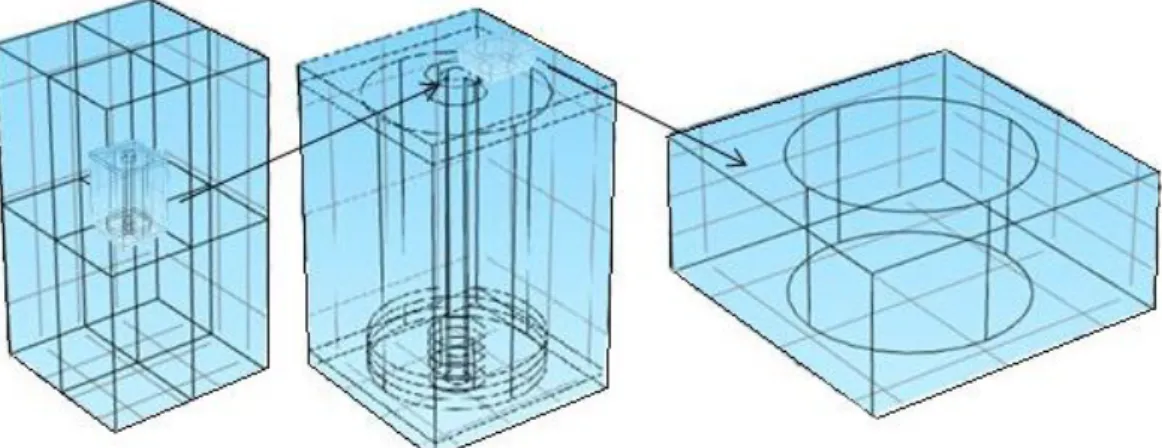
To briefly show how the original model was built and which the relationship between the three structural scales was, the text gives to the reader a simplified image, which does not respect the real size.

Figure 3: hierarchical model structure. The proportions do not respect the reality

The real novelty of this work is represented by the boundary conditions. In various examples, found in the scientific literature, such conditions are established by the operator depending on the analysis situation. On the contrary, in this case, the idea is to exploit the relationship between the macroscopic compression and the nanoscopic signal, which pushes cells to change in their architecture. With this goal the study starts at the macroscopic domain descending until the nanoscopic through the microscopic one. The mechanical model study is composed by several steps that will be exposed in the following paragraphs.

17

3.1 Longitudinal compression with vertical fibers: departing point

First the original model was analyzed to deep understand how it had been implemented. During the analysis and the plan to develop the study, several mistakes have been founded. Therefore the model has been corrected and completely remade.

First of all the analysis concentrates herself on a full vertical fiber specimen. Thanks to SiNuPrOs, physical characteristics have been obtained [12, 13 and 14]. The choice of a full vertical fibers specimen was not a random one. This direction is, in fact, the one in which fibers can at the best resist to a longitudinal compression stress. Such a stress is the most common simplified solicitation, a femur can be subjected to, during a usually activity as walking.

The size and the geometry adopted are briefly shown in the following scheme.

Figure 1[e]

Figure 4: this pictures shows how bone macroscopically is composed [5]

18

Figure 5: pictures (-i-), (-iii-) and (-v-) represent the various analysis physiologic steps, which have been modeled by the geometry in pictures (-ii-), (-iv-) and (-vi-). [1, 4, 5, 6, 7]

(-i-) (-ii-)

(-iii-) (-iv-)

19

SiNuPrOs™ is a computational system, which shows a graphic interface to the user, who can implement bone geometry characteristics and obtain tissue properties as elasticity matrix. In the back of that simple user interface, lots of hidden spreadsheets have been implemented.

By filling in information about geometry and percentage composition, data, as tensor matrix and compliance, can be obtained. These data would be used in an elaboration sheet of the macroscopic domain.

SiNuPrOs™ Fast allows evolution of cortical physical properties at macroscopic scale. The macroscopic domain, exploits the following data coming from SiNuPrOs™ (SiNuPrOs™ screenshot [13, 14]):

20

Two other dimensional scales are implemented: the microscopic and the nanoscopic ones. In the microscopic domain an osteonal structure is described. Data are filled in the relative spreadsheet to get the information, which are needed to implement the nanoscopic model part. In this one, an analysis of vertical collagen fibers can be found.

SiNuPrOs™ Fast Osteon allows evolution of osteonal physical properties at microscopic and nanoscopic scale. Since the analysis in this case is concerned with vertical fibers, the percentage of 100% of osteons 0-0 is inserted. The following data can be found (SiNuPrOs™ Fast Osteon screenshot [13, 14]):

23

3.1.1 Study at the macroscopic domain

The macroscopic domain contains five osteonal structures in each direction for a total of 125. In this case the osteons are not geometrically detailed. In any case the size takes in consideration their presence. In fact, four blocks of 390 µm x 390 µm x 715 µm (2 and ½ osteons) have been used to form a total cube composing the final block of 780 µm x 780 µm x 1430 µm.

Two physics are supposed to govern the medium behavior. The first one is the physic “Solids Mechanics”, which describes the solid part of bone.

Figure 6: screen capture from Comsol desk

The second one is the physic “Darcy’s law”, which describes the fluid part of bone. This one is related to the poro-elastic property of the analyzed material, which has two kinds of couplings. The fluid acts on the solid part by imposing a pressure contribute to the internal load of the solid. This one also acts on the fluid, because if the solid is compressed the holes dimension decreases and the fluid is ejected.The properties of the medium sample are anisotropic. These properties have been estimated thanks to the SiNuPrOs model [15, 16]. The Darcy’s law equation is the following:

Figure 7: screen capture from Comsol desk

24

In the solid mechanics physic the following conditions are imposed: o Body Load:

o Material properties: The elastic matrix is filled in thank to SiNuPrOs data [13,

25

14].

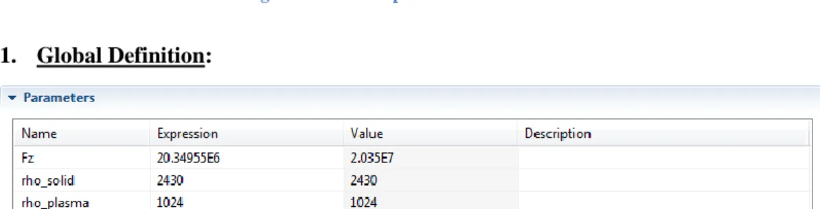
o Imposed charge: This part is obtained by imposing a load force Fz on the high

and low face. Fz has been chosen in order to respect a Von Mises stress of

20.35

MPa.

The applied load consists in a symmetric compression. In order to obtain it, the force has a sign minus in the case of the high face, and a plus for the low face.

x

z

y

26

o Prescribed displacements:

 First of all a null z-axe displacement for the median plane is imposed. Such a condition is coherent with the applied compression force. Logically this plane does not move, because in it the equilibrium between the two opposite forces is got.

Figure 10: displacement imposed to the middle plane

(-ii-) (-i-)

27

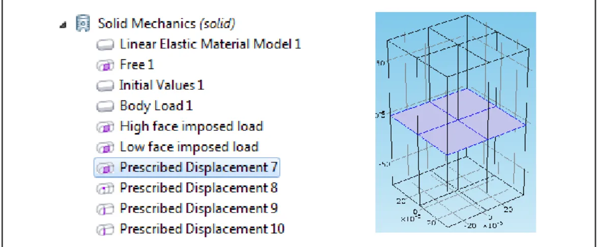
 Middle point displacement: The middle point is the only one that is not allowed to move at all.

28

 X- Horizontal line displacement: The horizontal line cannot move in z- and y-axe.

29

 Y- Horizontal line displacement: This line cannot move in z- and x-axe.

3. Darcy’s Law:

30

o Fluid and Matrix Properties:

o Initial Values:

31

o High Face Hydraulic Head: The pressure value occurring in the last picture has been determined in other study concerning the physical behavior of a complete femur (Rizzoli Institute, Bologna).

o Low Face Hydraulic Head:

32

o North-South Inflow Boundary: Figure 16: Low Face Hydraulic Head

33

o East-West Inflow Boundary:

35

3.1.2 Study at the microscopic domain

The macroscopic file is analyzed in specific points to insert such data in a following file, the microscopic one. The coordinates of the considered points are the ones shown in the table below.

P0 P1 P2 P3 P4 P5 P6 P7 P8 P9 P10 P11 P12 P13 x 0 -200 -200 -200 -200 0 -356 -356 -356 -356 -200 -200 --356 -356

y 0 -78 78 78 -78 0 -78 78 78 -78 -78 78 78 -78

z 143 143 143 143 143 -143 -143 -143 -143 -143 0 0 0 0

Table 1: coordinates of the points taken in the macroscopic model to obtain the boundary condition for the following model, the microscopic domain. The values are expressed in nanometers.

The displacements to impose in the microscopic domain are obtained thanks the elabora-tion sheet and the data, which had filled in.

In this context several equations have been built in order to find the adequate boundary conditions to impose in the following step. The equations have been built in accordance with a very simple principle (Annex A). Starting from the initial coordinates a general dis-placement equation is calculated thanks to disdis-placement information coming from the mac-roscopic computation. Generally speaking a face is schematized in (A, B) coordinates. In the figure below a scheme showing a development in terms of faces is shown.

36

In this case the coordinates, which are involved, have to consider the microscopic domain. Each face is observed by an external point of view and points are counted in the positive orientated sense, starting from the one in the up-right corner, in anticlockwise sense. In the table below each face and the corresponding points with their order can be observed.

Face

Points

North-High

4 − 3 − 11 − 12

North-Low

12 − 11 − 7 − 8

South-High

2 − 1 − 9 − 10

South-Low

10 − 9 − 5 − 6

West-High

1 − 4 − 12 − 9

West-Low

9 − 12 − 8 − 5

East-High

3 − 2 − 10 − 11

East-Low

11 − 10 − 6 − 7

High

1 − 2 − 3 − 4

Low

6 − 5 − 8 − 7

Table 2: order number to build the condition limit equations for a longitudinal compression case.

To simplify the notation, in accordance with the reference system, each face has been called with a cardinal name (N, S, E and W). With “high” and “low” the author wants to indicate the specific face part, in which the geometry has been cut.

P1

P2

P3

P4

P5

P6

P7

P8

P10

P9

P11

P12

37

An equation system has been built.

{

∝

𝑥𝑦 + ∝

𝑥 +∝

𝑦 +∝

= 𝑑

∝

𝑥𝑦 + ∝

𝑥 +∝

𝑦 +∝

= 𝑑

∝

𝑥𝑦 + ∝

𝑥 +∝

𝑦 +∝

= 𝑑

∝

𝑥𝑦 + ∝

𝑥 +∝

𝑦 +∝

= 𝑑

Where d1,.., 4 and α1,., 4 are the displacements coming from the macroscopic domain

compu-tation and α1,., 4 the coefficients the author was interested to estimate. (x, y) coordinates are

represented by the (A, B) combination points shown in the previous picture.

The operation has been made for each direction x, y and z and for each high or low face. The equations may present a great simplification in the case of z-coordinate, because the corresponding central point’s displacements are null. In this case, in fact, two α coefficients would be null. In any way, also in the others cases, simplified equations would be found, because of the null central point’s coordinates.

The general equations of a face defined by the points P1,.,P4 are shown in Annex A.

The obtained displacement equations are imposed as boundary conditions in the micro-scopic file model.

The physics, which are involved in the microscopic domain, are three: solid mechanics, Darcy’s law and Brinkman equation. Depending on the kind of the analysis, different kinds of equations combinations have been used. To describe the interstitial system and the oste-on, the physics solid mechanics and Darcy’s law are adopted. To model the fluid part in the Havers channel, Brinkman equation is used. The blood vessel in Havers channel is not modeled. Simply, a blood pressure defined as boundary condition, which is applied on a cylinder localized in the Havers channel, is considered.

1. Global definitions:

C_x, C_y and C_z coefficients have been introduced as multiplication factors of the displacements equations for the microscopic and the nanoscopic domain to uniform the stress in the different domain for each analyzed point.

38

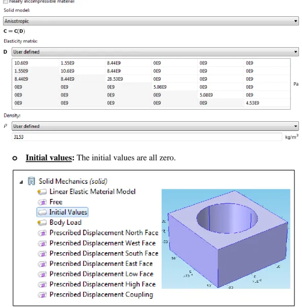
o Material properties: The matrix below has been built thanks to the SiNuPrOs™ Fast Osteon [13, 14] simulation program.

o Initial values: The initial values are all null.

39

o Volume charge: This charge shows the pressure contribution caused by Darcy’s law. The gravity effect is considered in the macroscopic domain.

o Imposed displacement: Since the appropriate spreadsheet, displacements are imposed to each face. For example, how a displacement can be imposed to the high face is shown.

The dimension is shown in order to be coherent.

3. Darcy’s law: The Darcy’s law physic involves several mass fluxes to apply to each

40

face and a coupling with the Brinkman physic, which would be describe in the following points.

o

o

o

41

The pressure value, occurring in the last picture, has been determined in others studies concerning the physical behavior of a complete femur (Rizzoli Institute, Bologna).

o

macroscopic data had been filled in, flux are imposed in the microscopic model.

For example, a displacement imposed to the high face is shown in the

picture below.

When data would be inserted in the microscopic model, the signs convention is important to observe.

42

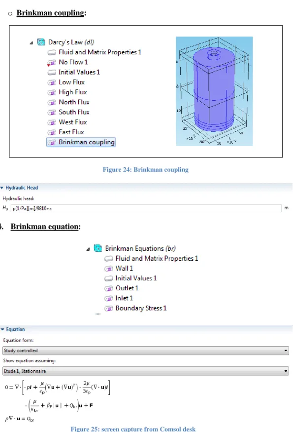
o Brinkman coupling:

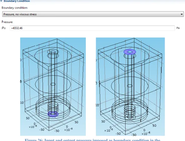
4. Brinkman equation:

Figure 25: screen capture from Comsol desk Figure 24: Brinkman coupling

43

o Fluid and matrix properties: The following properties are user defined as variables or as values.

o Initial values: The initial values are all zero.

o Entry and outgoing conditions: The pressure value given by the points 𝑃𝑖𝑛𝑝𝑢𝑡 and 𝑃𝑜𝑢𝑡𝑝𝑢𝑡 is taken. The points are the central points of the high and the low face.

44

o

Comsol found a problem with this coupling but, even if the author has look for it, any solution has been found. The physic has not been deleted, because the program

Figure 26: Input and output pressure imposed as boundary condition in the Darcy's law physic (microscopic domain)

45

converges.

47

3.1.3 Study at the nanoscopic domain

To obtain the conditions to impose to the model in the nanoscopic domain, some data are searched in some specific points between microscopic results. The coordinates in meter are the ones shown in the table below:

Table 3: coordinates of the points taken in the microscopic domain to obtain the boundary conditions to impose to the following model, the nanoscopic one. The values are expressed in meters.

Generally speaking, the nanoscopic domain is the analysis of a collagen fiber. The analyses can be either a vertical or a horizontal fiber. In the case of only 0-0 orientated fibers, the horizontal nano analysis does not have reason to exist.

Data about pressure, displacements and velocity field are the interesting ones. The boundary conditions to impose in the nanoscopic domain have been computed by applying the equation obtained in the same way described in paragraph 3.1.2. In this case the order points change as shown in the picture below.

Face

Points

4 − 3 − 7 − 8

2 − 1 − 5 − 6

1 − 4 − 8 − 5

3 − 2 − 6 − 7

1 − 2 − 3 − 4

6 − 5 − 8 − 7

Table 4: order number to build the condition limit equations for a longitudinal compression case.

To simplify the notation, in accordance with the reference system, each face has been called with a cardinal name (N, S, E and W).

The nanoscopic domain has five physics: solids mechanics, Darcy’s law, piezoelectric ef-fect and electrostatic. The two firsts have been introduced to schematized porous-elastic re-gions. A piezoelectric effect is to attribute to the collagen fibers and the electrostatic part is arose to model ions presence.

48

1.

C_x, C_y and C_z coefficients have been introduced as multiplication factors of the equations displacements for the microscopic and the nanoscopic domain to uniform the stress in the different domain for each analyzed point.

2. Solid mechanics:

49

o

50

o

coupling).

o

spreadsheet and filled in the nanoscopic file, as done in the preceding domain.

Figure 29: Body Load imposed to a vertical fiber

51

o

imposed.

Where u2, v2 and w2 are displacements, which would be obtained in the piezoelectric physics.

52

3.

o

53

o

o

version of Comsol, because it is neglectable.

o

The data imposed is expressed by a normalized x-axe velocity. In order to provide such entry flux, an x-axe velocity in the points defining the north face (

𝑃3 −

𝑃4 − 𝑃8 − 𝑃9

𝑣_0

o

are acquired from the osteonal study.

54

4.

The equations implemented are the following:

Figure 34: pressure imposition for the case of a vertical collagen fiber

Figure 35: piezoelectric physic for the case of a vertical collagen fiber

Figure 36: comsol screenshot. Piezoelectric equations.

55

o

reference [9].

o

56

o

.

o

coupling between the piezoelectric and the elastic problem is imposed.

𝑢

𝑣

𝑤

57

o

elastic-piezoelectric coupling, the same potential of the electrostatic problem is also imposed.

5.

nature.

The equations, that have been exploited, are the following.

58

Figure 40: screen capture from Comsol desk. Electrostatic equations.

o

o

o

59

o

Figure 43: external electric potential imposition for the case of a vertical collagen fiber Figure 42: null surface charge density for a vertical collagen fiber

61

3.1.4 Study of the piezo-electro effect

The analysis has been done in two coupling situations. In the first, all physic (solid, piezo, Darcy and electrostatic) are considered. In the second only the piezo- and electro- physics are simulated. The simulation proves the importance of the loading aspect. The piezoelectric represents the piezoelectric effect contribution, which is a characteristic of a collagen fiber.

Figure 44: nanoscopic results concerning the difference potential at the end of collagen fibers.

This one is important, because the text wants to investigate about the effect of a mechanical stress on the potential difference. Therefore, to demonstrate, that the found potential difference is not only coming from a resultant coupling with the solid and an electrostatic one, is important to show. By observing the previous pictures the author observed, that the piezoelectric effect is less than the other one. Therefore there is an evident mechanical effect.

Activated physic Solid-Piezo-Darcy-Electrostatic:

Max: 0.39007 µV

Min: -0.23671 µV

Activated physic Piezo-Electro:

Max: 0.0029287 µV

63

3.2 Transversal compression with vertical fiber: start of the model

development

The same work has been developed in the case of a transversal compression.

This phase consists in an analysis similar to the work already described. The boundary conditions, the direction of applied forces and the architectural conformation have been modified. A transversal compression has been implemented in the macroscopic domain.

The analysis goal is, as before, to explore the potential difference on the free boundaries surfaces of collagen fibers in the nanoscopic domain.

The data implemented as model input have been the same of [1] (paragraph 3.1). The changes will be analyzed in detail in the following paragraphs.

3.2.1 Changes

The original model has been modified by imposing a force compression along x-axe. In practice, in Comsol, the following steps have been followed to change the original configuration.

(-ii-)

Figure 45: pictures showing the way the compression forces act on the specimen in the two kinds of analyses the text talks about. Figure (-i-) shows a longitudinal compression and figure (-ii-) a transversal one.

64

Figure 46: north face to which a force Fz is applied.

65

In these pictures the charge of north and south parts is shown. The north part is outlined by 3 − 4 − 9 − 8 points and the south one by 4 − 5 − 6 − 7 ones.

The pictures below show the four changed prescribed displacement conditions.

66

Figure 49: middle point to which a prescribed displacement is applied

67

The physics “Darcy’s law” has not been changed compared with the macroscopic analysis in a longitudinal compression.

Another important change to remark is the one led to the condition limits equations to impose to the microscopic model. The microscopic geometry has been split in a vertical direction in spite of a horizontal one. The same choice has been made for a flexion stress. Such analysis will be described in the following paragraphs.

68

The new split configuration is shown in the picture below.

The macro-micro spreadsheet has been changed in accordance with the equations shown in Annex 2. The points, where data had been acquired, in the macro domain are the following:

P0 P1 P2 P3 P4 P5 P6 P7 P8 P9 P10 P11 P12 P13 x 0 -200 -200 -200 -200 0 -356 -356 -356 -356 -278 -278 -278 -278

y 0 -78 78 78 -78 0 -78 78 78 -78 -78 78 78 -78

z 143 143 143 143 143 -143 -143 -143 -143 -143 143 143 -143 -143

Table 5: coordinates of the points taken in the macroscopic domain to obtain the boundary conditions to impose to the following model, the microscopic one. The values are expressed in meters.

The nanoscopic domain did not require any change from the geometry point of view. The input information about pressure and displacement field coming from the preceding files have had the necessity to be modified. The author proceeded in the same way as in the case of a longitudinal loading.

69

3.2.2 Study of the piezo-electro effect

The potential difference coming from the nanoscopic domain is shown in the picture below for a transversal compression in two difference coupling situations.

Figure 52: nanoscopic results for a transversal compression in two different coupling situations.

The piezoelectric effect is less than the mechanical one for the first two analysis cases. The resulting potential difference derives only from the piezoelectric effect induced by the solid

.

3.2.2 Comparison between longitudinal and transversal compression

From a preliminary analysis a difference in terms of PD has been observed. For a longitudinal compression a PD of 6.2678E-7 V has been obtained and for the transversal one about 3.21784E-8 V.

Between the longitudinal and transversal compression of fibers 0-0 there is difference of a factor 20. It is coherent with the fact that the PD is a possible signal to start the remodeling phenomenon.

The next step of the analysis has been the implementation of various architectures (depending on osteon nature) analyses both for the longitudinal both for the transversal compression. Data will be discuss in detail for all kind of implemented architectures in

paragraph 3.4.

The results coming from the computation are shown in the following tables.

Activated physic Solid-Piezo-Darcy-Electrostatic:

Min: 0.0

Max: 0.00

Activated physic Piezo-Electro:

Max: 0.0029287 µV

70

Vertical [V]

Horizontal [V]

(min, max)

PD

(min, max)

PD

Longitudinal

compression

0-0

6.2678E-7

0-90

3.3073E-7

4.0198E-7

6.315E-7

-1.1446E-7

-2.2055E-7

O

1.23696E-7

4.231E-7

-1.0193E-7 -3.2567E-7

90-90

2.455E-7

-8.3078E-7

Table 6: results in terms of potential difference for transversal compression

Vertical [V]

Horizontal [V]

(min, max)

PD

(min, max)

PD

Transversal

compression

3.2178E-8

0-90

3.4274E-8

4.865E-6

1.1305E-9 -2.4024E-6

O

3.0966E-8

5.335E-6

1.1598E-9 -2.1457E-6

90-90

3.865E-6

-1.9059E-6

Table 7: results in terms of potential difference for longitudinal compression

By comparing all the results coming from an analysis of different kinds of fibers for a longitudinal and transversal stress, an incoherence came out. The longitudinal compression does not show any relevant difference between the different kinds of fibers. In the case of a transversal compression, the horizontal fibers show the PD about 1µV versus a 0.01µV for the vertical fibers.

Probably a full longitudinal stress is not a good physiological representative one. Probably, an human femur does not allow a completely vertical applied stress. The suggested idea has been that such a stress is a too much big simplification of the biological loading applied on a bone specimen. In fact, a femur is not subjected to a completely vertical compression, but also to a horizontal force. The analysis has been, then, modified to simulate a flexion stress.

71

3.3 Flexion

This kind of analysis has required a modification in the imposed displacements and in the kind of force to apply in the macroscopic domain. Moreover, as consequence of the modification of the imposed displacements, also the boundary condition equations to fill in the microscopic model spreadsheet have been necessary to modify.

The changings in the macroscopic domain have consisted in an imposition force (0.1 of the longitudinal force) in the horizontal direction (x-axe).

Figure 53: high face load for a flexion case

72

In order to respect the physic of a flexion stress a null z- and y-displacement to the middle (xy)-plan and a total null displacement to the middle point have been imposed. Moreover a y null-displacement to the middle (xz)-plane has been imposed.

Figure 55: imposed displacement to the median plane for a flexion case

73

After the macroscopic computation, the author, by observing the stress distribution on the specimen, has detected a parabolic distribution of stress. That is why an analysis in 14 points for the microscopic domain, as the one lead in the case of a longitudinal stress, has been necessary. The same kind of equations of the longitudinal case have been taken, but since the imposed displacements have been changed, also the equation had to. The limit condition equations are shown in Annex C.

The microscopic and nanoscopic domains did not have any change compared to the others implemented cases.

75

3.3.1 Potential difference coming from the nanoscopic domain in a

flexion stress analysis

The results obtained, by imposing a flexion, stress may be resumed by the picture below:

In this case the analysis is satisfactory. The PD relevant increases than the one in a longitudinal stress applied on 0-0 full fibers specimen. The author tried, then, to look for others kinds of architecture. The next analyses have been described in the paragraphs below. The author implemented also a standalone program to simplify the multiscale model implementation. This one would be described at as the last one.

Activated physic Solid-Piezo-Darcy-Electrostatic:

Max:

Min:

77

3.4 Others architectures

Starting from these preliminary results, others kinds of architectures have been analyzed in order to confirm what said. The different kinds of analyses are shown, with the name of each file they are composed of, in the list below.

78

In the macroscopic, microscopic, and nanoscopic domain, data have been changed in order to respect the new architectures. The following pictures show the data adopted in each analyses case. Each table represents a SiNuPrOs screenshot. The geometry is the same shown in paragraph 3.1.

79

Macroscopic general geometry:

80

Case of the presence of 100% O orientated fibers:

81

82

83

The reader could ask himself why there exist so many osteons. That is why the

microscopic model consists in the analysis of a single osteon. The analysis split in different parts is necessary. A part for each osteon, which composes the architecture. Moreover each osteon file has one or two corresponding nanoscopic files. In fact, even if the geometry and the data are the same, there exist two different files to describe horizontal and vertical fibers. Depending on the fiber type contained inside the osteon, the analysis may require a vertical or a horizontal or both studies. The relationships between the microscopic and the nanoscopic domains to consider are briefly shown below

:





 Osteon 0-90: both vertical and horizontal fibers  Osteon O: both vertical and horizontal fibers

In the case of a horizontal fiber, the analysis in the nanoscopic scale is as the one already seen for the case of a vertical fiber. Since now a different fiber is implemented, also a different geometry must be considered.

84

The physics impositions are very similar to these already explained in paragraph 3.1 and 3.2, but these have been changed in order to respect the new geometry configuration.

Figure 61: initial values to impose to a horizontal fiber

85

Figure 63: example of imposed displacement for a horizontal fiber (north imposed displacement)

86

Figure 65: physic Darcy's law

87

Figure 67: pressure imposition for the case of a horizontal fiber

Figure 68: velocity imposition for the case of a horizontal fiber

88

Figure 70: null charge for the case of a horizontal fiber

Figure 71: initial values for the case of a horizontal fiber

89

90

Figure 74: electrostatic physic for the case of a horizontal fiber

91

Figure 77: external electric potential imposition for the case of a horizontal fiber Figure 76: charge density imposition for the case of a horizontal fiber

93

4. Matlab-Comsol implementation

ModelImplementation.m

User



Configuration ?



Analysis type ?

macro_model.m

saves data in file.dat)

SiNuPrOs

02 Excel spreadsheet

1 writes the percentage configuration in the SiNuPrOs file. Then it reads the resulting elastic matrix and call the macro_model.m file by giving him the information about the chosen architecture and the analysis case.

1 loads macro data and writes such information in the 02 Excel spreadsheet, whose name depends on the analysis case.

END

1 implements a “for cycle” to compute the micro and the nano model scales. Four elastic matrices are defined. In the “for cycle” the initial architecture vector, chosen by the user, is analyzed. For each osteon kind the micro_model and the nano_model are called by specifying the elastic matrix

and the case of analysis.

04 Excel

Spreadsheet

micro_model.m

saves data in file.dat)

Transcription.m

nano_model_vert.m

nano_model_horiz.

m

This phase concerns both the loading of the limit conditions equation both the computation of the nano

94

Once the multiscale model, the text talked about, has been verified, the author implemented a Matlab program in order to simplify the used model.

The programming environment has been Comsol Multiphysic 4.2 linked with Matlab. The author adopted both a technique of reverse engineering by exporting Comsol file and by implementing them in Matlab code, both loading Comsol file from Matlab function and by modifying them. This kind of approach is due to the complexity of the program, it has been necessary to implement.

The program is composed by:

1) SiNuPrOs file: file which allows the user to choose a fiber architecture configuration. It is a standalone program, to which the user can access thanks to the

ModelImplementation.m file. The instructions given during the computation have to be

followed. The user can access to the fiber configuration only in this step study. The dimension is fixed and cannot be changed, because the access to the micro and nano architectural data is not previewed. For that reason the advice is to not change anything in the data filled in SiNuPrOs datasheet. In the contrary case, to change data in the others Matlab files would be necessary, but most of all changing the defined geometry of the Comsol model file.

2) ModelImplementation.m: m-file interacting with the user by video string messages. It is the responsible of the interaction between the several parts, the program is composed of. In this phase the user can choose the kind of architecture to analyze and the type of stress to apply to the specimen.

An important remark is, that this program has been implemented mainly for the following case:

2. a) longitudinal stress 2. b) transversal stress 2. c) flexion stress

The user has not to change the files, because the program will give an error message and will stop. Previous developments for such a program would be the extension to all possible analysis cases. How to properly implement them is really important, because the limit conditions and the micro file depend from the stress the user decides to apply to the specimen.

95

arguments an elastic matrix and a variable n indicating the case 1), 2) or 3) of the stress configuration.

4) micro_model.m: matlab function developing the micro analysis. This function has as arguments an elastic matrix and a variable n indicating the case 1), 2) or 3) of the stress configuration. This file contains a code, which accesses to a Comsol 03 file, and modifies it. After the modification a message would be displayed. Such a message invites the user to compute the micro file opening Comsol environment. This kind of choice has been taken, because this file takes too much time to turn in Matlab.

In Comsol 300-600 seconds would be necessary the program to turn. After that, the user has to save the 03 Comsol file and to close it. Then, he has to push Enter and the Matlab analysis will prosecute.

5) Transcription.m: matlab function loading the micro data and writing them in the 04 excel datasheet for the following nanoscopic analysis.

6) nano_model_vert.m: matlab function developing the nano vertical analysis. This function has as argument an elastic matrix built in the ModelImplementation.m.

After the computation, the program returns. If the user would like to make previous analyses, he has to consider that the obtained data will be subscribed. Then, he has to copy them in another folder to save the work.

7) nano_model_horiz.m: matlab function developing the nano horizontal analysis. This function has as argument an elastic matrix built in the ModelImplementation.m.

After the computation, the program returns. If the user would like to make previous analyses, he has to consider that the obtained data will be subscribed. Then, he has to copy them in another folder to save the work.

For a more detailed description of the Matlab-Comsol implementation, the reader has to read the code of the described program.

97

5. Results

The analysis results coming from the Matlab-Comsol model computation are

shown in the tables below:

Vertical [V]

Horizontal [V]

(min, max)

PD

(min, max)

PD

Longitudinal

compression

0-0

6.2678E-7

0-90

3.3073E-7

4.0198E-7

6.315E-7

-1.1446E-7

-2.2055E-7

O

1.23696E-7

4.231E-7

-1.0193E-7 -3.2567E-7

90-90

2.455E-7

-8.3078E-7

Vertical [V]

Horizontal [V]

(min, max)

PD

(min, max)

PD

Transversal

compression

3.2178E-8

0-90

3.4274E-8

4.865E-6

1.1305E-9 -2.4024E-6

O

3.0966E-8

5.335E-6

1.1598E-9 -2.1457E-6

90-90

3.865E-6

-1.9059E-6

Vertical [V]

Horizontal [V]

(min, max)

PD

(min, max)

PD

Flexion

0-0

3.2997E-5

-2.5743E-5

0-90

7.5341E-7

4.493E-6

-4.0143E-7 -2.3288E-6

O

2.9579E-5

9.167E-5

-1.4001E-5 -4.5231E-5

90-90

5.768E-6

99

6. Conclusion

By comparing the data obtained in the analyses we can conclude that:

1. The piezoelectric effect is less than the mechanical one for the longitudinal and

transversal analysis cases. That is really important, because the analysis wants to investigate about a mechanical effect. The resulting potential difference derives only from the piezoelectric effect induced by the solid.

2. Between the longitudinal and the transversal compression of fibers 0-0 there is

difference of a factor 20. This result is consistent with the fact that the PD is a possible signal to start the remodeling phenomenon.

3. By comparing all results coming from an analysis of different kinds of fibers for a

longitudinal and a transversal stress an incoherence came out. The longitudinal compression does not show any relevant difference between the different kinds of fibers. In the case of a transversal compression, the horizontal fibers show the PD about 1µV versus a 0.01µV for the vertical fibers. The incoherence is in the longitudinal compression.

4. Probably a full longitudinal stress is not a good physiological representative one.

Probably an human femur does not allow a completely vertical applied stress. In fact, there is not a so relevant difference between the PD coming from different kinds of fibers loaded with a longitudinal compression. The conclusion is that a femur does not allow a completely vertical applied stress.

5. In the case of a flexion stress the situation gets more complicated. In the case of

uncoupled fibers, the vertical ones are the preferred with a PD about 10µV. This result confirms the point 3. Such a PD value, in fact, is bigger than the corresponding in a transversal compression. It is another proof of the role of the PD signal as the leader of the remodeling phenomenon.

6. The flexion stress is different from the other kind of stress. In such a bone load, also

the horizontal fibers would be solicited. In this case, in fact, the 90-90 fibers show a relevant PD of the same order of a transversal compression. Moreover a flexion stress shows the greatest results in terms of PD with the coupled fibers. In particular, the case of O fibers is to remark. This one shows a 10µV value for each orientated fiber. This indicates that the preferred case is the coupled one. There is any preference for vertical or horizontal one in this case, but they both are of the same order of magnitude.

101

7. Future developments

Certainly the model, exposed in this text, needs a magnification in terms of the implemented code to integrate more analysis cases. After that, an experimental validation both of SiNuPrOs simulation program both of the bone remodeling model would be necessary. In fact, choices, as the one to uniform the stress in different domains by multiplying the displacement equations, would be disputable.

The described model is only a mechanical one. The biological integration would be make it complete and useful in the bone application domain.

103

Acknowledgements

The development of this work has been possible thanks to of lot of factors. First of

all I want to thank the Professor Jean-Marie Crolet, my French supervisor, who has

led my project and organized my foreign experience.

Moreover I would like to thank Mihaela Racila, University of Cracovia, for her

disponibility during all the exchange period. She has made possible the

computation of all the files thanks to her opétron. Without her help any results

would be obtained and the project would not finish.

I thank also my Italian supervisor, Luca Cristofolini, Massimiliano Baleani, the

Erasmus LLP organization and the ISIFC Institute (Institut Supérieur d’Ingénieurs

de France-Comté) for the performing experience they gave me the possibility to

make.

Finally, I thank also all people who sustained and encouraged me during this

experience.