Performance of a new set of Micro-windows for the retrieval of Pressure, Temperature, Water and Ozone from MIPAS observations

(1)

University of Bologna

Faculty of industrial Chemistry

Atmospheric Physical Chemistry group of the

Department of Inorganic chemistry and physics

Master Thesis

Advanced Spectroscopy in Chemistry

Performance of a new set of Micro-windows

for the retrieval of Pressure, Temperature, Water

and Ozone from MIPAS observations

NAVE ANDY

Tutor: Co-Tutor: Prof. Dr. MASSIMO CARLOTTI ENZO PAPANDREA

(2)

Summary:

The framework of this thesis is the study of the atmosphere thanks to the MIPAS instrument (Michelson Interferometer for Passive Atmospheric Sounding) on board of ENVISAT (Environmental satellite). MIPAS is a spectrometer designed by the European Space Agency to measure broad-band spectra of the atmosphere from space in the mid-infrared range. However, small spectral intervals are used to retrieve the altitude distribution (profile) of several targets (level 2 product). These spectral intervals, called Micro-Windows (MWs), are selected in order to maximize the information content and minimize the total error of the level 2 products at all the retrieval altitudes.

The first objective of this thesis was to compare the performance of two sets of MWs; one provided by the University of Bologna (8 MWs) and the other by the Oxford University (10 MWs) for the simultaneous retrieval of Temperature, Pressure, Water and Ozone. For this purpose I retrieved altitude profiles on simulated observation from the two sets of MWs for the above geophysical targets and for the other main targets (Nitric Acid, Methane, Nitrous Oxide and Nitrogen Dioxide) that are determined downstream in the retrieval chain making use of the previously retrieved profiles. The retrieval has been performed with the analysis code, called GMTR, that is based on the Geo-fit approach (tomographic retrieval) along with the Multi-Target Retrieval (MTR) functionality (interfering species retrieved simultaneously).

The strategy of simulated retrievals permits to know the reference atmosphere so that it becomes possible to compare the retrieved profiles with the reference profiles. Thanks to specific quantifiers, that I defined for the purpose, I plotted and compared easily the performance of the two sets of MWs. The result was that the Oxford set of MWs has a better overall performance.

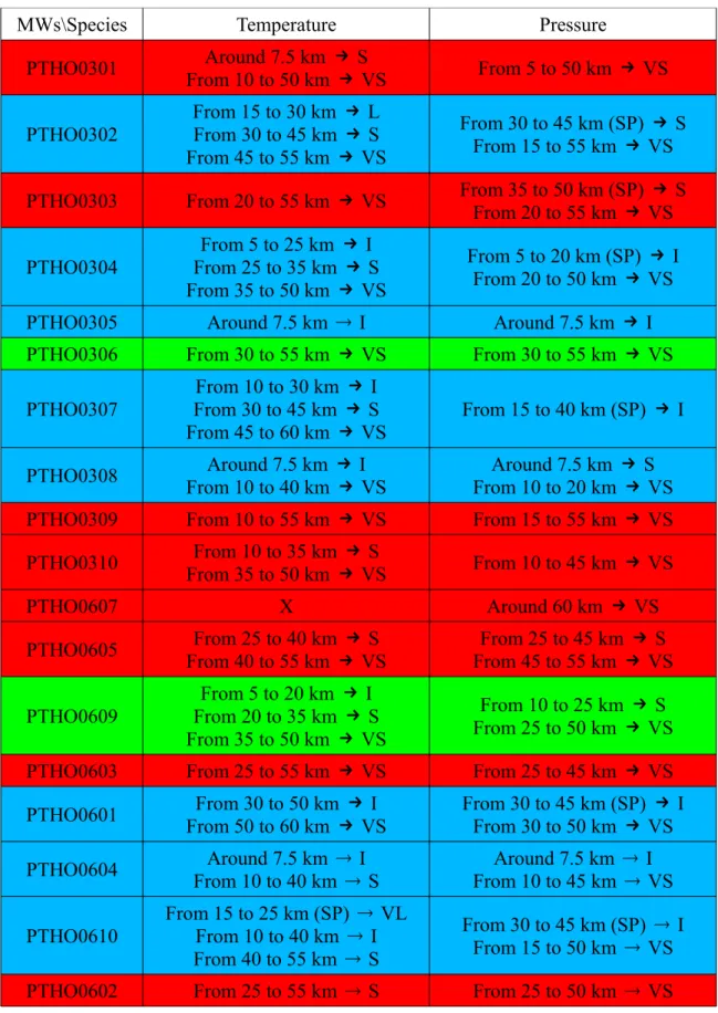
The two sets of MWs were then compared using a recently developed diagnostic tool called Information Load (IL). I computed and compared the IL values of the two sets of MWs for the four main targets (Temperature, Pressure, Ozone and Water). The IL distributions miss a full coverage of the atmosphere for both sets of MWs; therefore I decided to merge the best elements of each set with the aim of obtaining a more uniform IL coverage. In order to select an optimal set I computed the IL values for each individual MW. A combined set of MWs was then created trying to cover all the atmosphere with the highest possible amount of IL. After several attempts I selected a set of 10 MWs (combined set). The IL distributions of the combined set are better than those of the original sets for all targets excepted for Pressure around 50 km of altitude.

I tested the performance of the combined set of MWs with the strategy of retrievals on simulated observations: by comparing the performance of the profiles obtained using the combined set with the performance of the corresponding profiles obtained from the Bologna and Oxford sets, I verified an overall better efficiency of the combined set with respect to both the other two at low altitudes and equal or worst efficiency at high altitudes.

I compared the performance of the three sets of MWs by retrieving the eight MIPAS main targets from a statistically meaningful set of real observations. In this case the estimated standard deviation (ESD) of the retrieved values (calculated by the retrieval algorithm) provides the comparison criterion: I found lower ESDs for the combined set of MWs excepted for Pressure above 40 km.

Finally I considered the systematic error components (that are provided for each set of MWs by the selection algorithm) and I calculated an estimate of the total error for the three sets: the combined set of MWs has slightly lower total error at low altitudes and generally higher error at high altitudes.

(3)

A further meaningful element to be kept in consideration is the computing time: the Oxford set of MWs (that was a generally better efficiency than the Bologna set) requires between 13 and 15 hours of CPU time to analyse on orbit of MIPAS measurements, the Bologna set requires between 3 and 5 hours while the CPU time for the combined set is between 9 and 11 hours.

(4)

Introduction:

The framework of this thesis is the study of the atmosphere. In this scope spectroscopic instrument placed on board of artificial satellites are recording spectra of the atmosphere. These spectra are mainly used to retrieve altitude distribution of several targets (Temperature, Pressure and the main chemical components of the atmosphere). To avoid the redundancy of information and to save computer time, the retrieval process extracts narrow spectral intervals from the spectra. The retrieval process is currently using a set of spectral intervals selected by the University of Bologna. A new set of spectral intervals has been provided by Oxford University. The objectives of this thesis are the assessment of benefits and drawbacks of these two sets of spectral intervals and the merging of these two sets to create a “combined” set which should combine the benefits and discards the drawbacks.

Outline:

In Chapter 1, I describe the Environment Satellite and the inboard spectroscopic instrument, the Michelson Interferometer for Passive Atmospheric Sounding. This Spectroscopic instrument has the main assignment to extend our knowledge of atmospheric chemistry.

In Chapter 2, I introduce the so called Inverse Problem that is the problem of finding the best representation of the required parameters from measurements that are a complicated function of the parameters.

In Chapter 3, I briefly describe the retrieval process which retrieves from the MIPAS recorded spectra, the altitude profiles of Temperature, Pressure, and the main chemical components of the atmosphere.

In Chapter 4, I describe the diagnostics tools which are needed and will be used in the subsequent chapters to complete the analysis of the spectral intervals of the two provided sets, i.e. the retrieving of altitude profiles on simulated observations, the Information Load and the Systematic and Random errors.

In Chapter 5, I describe and use the quantifiers which are employed to compare the retrievals on simulated observations for Temperature, Pressure, Ozone, Water, Nitric Acid, Methane, Nitrous Oxide and Nitrogen Dioxide of the two sets of spectral intervals.

In Chapter 6, I compare the Information Load values retrieved thanks to the two sets of spectral intervals. Then I retrieve the Information Load for each individual spectral interval to select the most efficient and so create a more efficient, combined set of MWs.

In Chapter 7, I compare the combined set of spectral intervals in front of the two primary sets using retrievals on simulated and real observations. Then I finish the comparison looking at the systematic and total errors.

(7)

1 The MIPAS experiment

1.1 ENVISAT

The Michelson Interferometer for Passive Atmospheric Sounding (MIPAS) is on board of the ENVIronmental SATellite (ENVISAT), it is an advanced polar-orbiting Earth observation satellite developed by the European Space Agency (ESA) that was successfully launched on a nearly polar orbit on 1 March 2002. The ENVISAT payload consists of a set of ten instruments (whose MIPAS) that operate over a wide range of the electromagnetic spectrum, from centimetre waves to the ultraviolet. This satellite provides measurements of atmosphere, oceans, lands, and ice and contributes significantly to extend our knowledge of climate and morphology of our planet. [1]

1.2 The MIPAS instrument

The MIPAS instrument is based on a Fourier Transform spectrometer that performs limb sounding observations of atmospheric emission in the middle and upper atmosphere. MIPAS observes the Earth's horizon measuring a wide spectral interval in the infrared region where many of the atmospheric trace-gases have important emission features. MIPAS observations are independent from sun position, then allowing continuous measurements, also during night or polar winter. The combination of high spectral resolution, full coverage of the mid-infrared region, high sensitivity, and full global and seasonal coverage, provide unprecedented insights into chemistry and dynamics of the atmosphere. [2], [3]

1.2.1 The characteristic of the MIPAS instrument

The MIPAS instrument is similar to an ordinary Michelson Interferometer, except some modifications that were made to adapt it to operate on board of a satellite with a high sensibility. Some of these modifications are:

• The use of two movables mirrors, instead of one, to reduce the dimension of the instrument.

• These mirrors are moving in opposite direction in two parallel pathway, rather than perpendicular, to not confer to the orbital station a rotational moment when occurs the reversal of movement of the two reflective elements (see Figure 1.1).

• The use of a laser beam to obtain a high precision in the displacements of the moving elements

• Maintain all the optical elements at a temperature of 200 Kelvins, to reduce their thermal emission

• The use of a series of eight detectors Hg:Cd:Te, cooled at 70 Kelvins.

• The use of the radiation emission by a black body to a known temperature, for the radiometric calibration.

(8)

1.2.2 Measurement description

The main purpose of MIPAS is the measurement of the distribution in altitude (profile)

of Temperature and Pressure, as well as the volume mixing ratio (VMR)1_{of numerous}

species like water, ozone, nitric acid, methane, nitrous oxide, and nitrogen dioxide.

To obtain these results, MIPAS measures the emission of the atmosphere using the technique of “limb scanning”, which consist in repeated measurement with different geometry of observation which not encounter the Earth's surface. Figure 1.2 shows a scheme describing the technique of limb scanning for a satellite. In this example, the orbital station flies at a altitude Hf, and performs with different angle ϑi, various measurements, which of them is characterise by the tangent altitude Hi, which is the minimum altitude reached by the line of sight.

1_{The VMR (volume mixing ratio) is define as the ratio between the number of molecules of}

a tested species and the total number of molecules present in the same volume.

(9)

A, B, C Line of sight Hf = Flight Altitude Hi = Tangent Altitude

Li = Stratification of the atmosphere ϑi = Zenith Angle

1.2.3 The characteristic of the original MIPAS experiment

MIPAS provides series of spectra at different tangent altitude, the system operating the instrument MIPAS allows to scan between the altitude 5 to 150 km. Normally, a sequence of limb-scanning provides 16 spectra, takes 75 seconds (corresponding to a movement of the satellite of about 530 km), varying the tangent altitude from 6 to 68 km, where the studied species have the most important abundance.

Depending on the scientific objective, the “special” observation modes may differ from the “nominal” mode (see table 1.1) as these parameters: the adopted spectral resolution, the altitude coverage, the vertical/horizontal sampling steps, or the azimuth direction of the line of sight.

For one scan, the field of view is only of 3 km in altitude, to obtain a good vertical resolution, and is large of 30 km, to receive enough energy.

The usual measurements are in the opposite direction of the satellite movement. In special cases, it is possible to carry out the measurements in the perpendicular direction of the satellite flight, in the opposite direction of the sun. This mode is very useful to observe particular phenomena, as volcanic eruption, control of the pollution on the major air routes, or support eventual campaign of regional measurements.

The distance between the instrument and the tangent altitude is of about 3300 km. To obtain measurements on the desired line of view is necessary to effectuate an accurate calibration of the pointing system, which will takes the stars position as reference. The

spectral interval of this instrument covers the mid-infrared: from 685 cm-1_{to 2430 cm}-1_.

One complete spectrum is obtained in 4.5 seconds, with a resolution of 0.035 cm-1_{. Of}

course, it is also possible to effectuate measurements with a reduce spectral resolution, in a reduce time of acquisition. In Figure 1.3 are reported the mains parameters of the MIPAS observation.

(10)

Observation

Mode Scientific Objective

Pointing Direction Coverage Altitude Range (km) Height Resolution (km) Horizontal Spacing (km) Nominal chemistry and Stratospheric

dynamics

rear Global 6-68 3-5-8 530

Polar Winter Chemistry

Polar Chemistry and

Dynamics rear Global 7-55 2-10 420

Tropospheric Stratospheric Exchange Exchange between Stratosphere and Troposphere, Troposphere Chemistry rear Global 5-40 1.5-10 420 Impact of Aircraft Emission

Study of major air

traffic corridor side

Primarily North of 25° latitude 6-40 1.5-10 330 Stratospheric Dynamics Small scale structures in the middle Atmosphere rear Global 8-53 3 390 Diurnal Changes Diurnal changes

near the terminator side

Near the

terminator 15-60 3 480

UTLS Troposphere / Upper

Lower Stratosphere

rear Global 6-35 2-7 120

Upper

Atmosphere Upper atmosphere rear Global 20-160 3-8 800

Table 1.1: MIPAS nominal and special observation modes (before March 24, 2004)

(11)

1.2.4 Data Processing

MIPAS Interferometric measurements are transformed into calibrated spectra of atmospheric radiance. The spectra are fed to an inversion model to compute vertical profiles of atmospheric geo-physical parameters. From the most raw interferograms to the final atmospheric profiles, there is series of necessary processing steps. The processing chain is separated in two major parts: a “space segment” and a “ground segment”. The flowchart in Figure 1.4 illustrates the flow of MIPAS processing.

Data acquired in orbit by the instrument are transmitted to ESA ground stations where undergo further stages of processing, resulting in higher level data products. The ground processing is divided into two major processing phases: Level 1B and Level 2 processing. The goal of the Level 1B processing is to decode the instrument source packets and transform the interferograms into calibrated spectra of atmospheric radiance, with correction of the Doppler effect due to the movement of the orbital station . This process has also for purpose to obtain the tangent altitude and the geolocation of the data. In the subsequent Level 2 processing phase, the calibrated spectra are processed by ESA to retrieve atmospheric pressure at tangent altitudes and vertical distribution of temperature and VMR of relevant atmospheric constituents. All the resulting data products are delivered in a format specific for the ENVISAT Ground Segment (Payload Data Segment – PDS) and are identified by labels indicating the step in the processing chain.

(12)

MIPAS Level 0 data correspond to the data stream received directly from the

instrument without any further processing.

MIPAS Level 1A data are intermediary data, not archived or distributed, used as

starting point for the subsequent processing stage.

MIPAS Level 1B data consist of formatted, geolocated, radiometrically and spectrally

calibrated radiance spectra, also annotated with quality indicators.

MIPAS Level 2 data comprise retrieved profiles of Pressure, Temperature and VMR of

H2O, O3, HNO3, CH4, N2O and NO2.

1.2.5 Current status of the MIPAS instrument

MIPAS started working successfully since April 2002. The measurement campaign proceeded with only few interruptions due to various types of anomalies experienced by the interferometer unit. All these anomalies pointed to a degradation of the interferometer subsystem, but MIPAS scientific return was not affected: the generated products were still meeting the engineering and scientific requirements.

On March 26th_{, 2004 MIPAS regular operations were suspended for a serious anomaly}

related to an unexpected behavior of the interferometric mirror slides. An exhaustive series of tests was carried out in order to identify the cause. The analyses highlighted a combination of different effects, the most important being a mechanical degradation of the interferometer slides. This anomaly did not allow to operate the instrument in its original configuration.

During the unavailability period, MIPAS was tested in different operational modes in order to assess the safer one with respect to the instrument health and to continue in the production of data with the best quality, i.e. “2RR” double-slide moving mirrors with a reduced resolution of 0.0625 cm-1_{, and the “1RR” single-slide moving mirror with a}

resolution of 0.05 cm-1_{. Amongst the possible configurations, the MIPAS Science Team}

decided to operate the instrument for the future in the more stable double-slide mode in

which the spectral resolution is to be kept at 0.0625 cm-1_{, that is 41% of the full spectral}

resolution used in the original nominal configuration. The instrument was operated in discontinuous way and the data quality was marginally affected. In Table 1.2, is described the new parameters associated to the observation mode, modified to match the reduced resolution.

Although it was evident that the anomaly was caused by a mechanical problem, the precise cause is still not fully understood. An empirical understanding is that the interferometer performance improves after a long period of interruption.

From January 2005 to December 2007, MIPAS was back in operation working with the measurement scenario of 3 days-on and 4 days-off. This scenario allows a global coverage to be obtained in the three days of operations, while the four days switch-off of the instrument is request for relaxing the interferometer slides system.

Between January 2005 and December 2007, the instrument operated on a 35% duty cycle but since December 2007 has been operating full-time with a standard 10 day sequence of 8 days nominal mode, 1 day MA, 1 day UA. [4], [5]

(13)

Observation

Mode Acronym Description Coverage

Altitude Range (km) Scans Numbers Horizontal Spacing (km)

Nominal NOM chemistry and Stratospheric

dynamics Global 5-77 27 410 Upper Troposphere / Lower Stratosphere

UTLS-1 Primary UTLS _mode Global 5.5-55 19 290

Upper Troposphere /

Lower Stratosphere

UTLS-2 Test mode for 2-_{D retrieval}

Global (limited numbers of orbits) 12-42 11 180 Middle Atmosphere MA Exchange between Upper Atmosphere and stratosphere Global 18-102 29 430 Middle/Upper atmosphere in summer NLC Detection of Noctilucent clouds in the Polar Summer North and South pole during polar summer 39-102 25 375 Upper Atmosphere UA Measurement high altitude NO and temperature Global 42-172 35 515 Aircraft Emission AE Study of major air traffic corridor Primarily North of 25° latitude 7-38 12 n.a.

Table 1.2: MIPAS nominal and special observation modes (after December 1, 2007)

The 8 April 2012, the contact with ENVISAT has been lost and all attempt to re-establish the communication has been unsuccessful. The ENVISAT satellite has already doubled its expected operations lifetime.

(14)

2 The Retrieval Problem

As I explained in chapter 1, the main objective of the MIPAS experiment is to obtain the altitude profiles of several targets relevant to the study of the atmosphere. The problem of retrieving the altitude profiles from the measured spectra is known as the Inverse Problem [3]. There exists a large amount of literature on this subject, both from the mathematical point of view and applied to specific scientific problems. A very good textbook for Remote Sensing retrievals is [6]. The notation and concepts introduced in this chapter are inspired to those described there.

2.1 The problem

In accordance with convention, the collection of values to be retrieved is referred to as the state of the atmosphere that we usually denote with x. The forward problem is the mapping from the state of the atmosphere to the quantities that we are able to measure. The details of the forward problem is in our case given by the physical theory of the atmosphere. The forward mapping may be linear or non-linear and is denoted by F. In practice we are never able to make exact measurements and the data that we actually measure are a corrupted version of the error-free data obtained through the forward process from the state of the atmosphere. The difference between error-free data and the measured data, denoted by y, is called the measurement noise and is denoted by ε. Thus the mapping from the state of the atmosphere to actual data is given by the relation: “y = F(x) + ε”. The inverse problem is then the problem of finding the original state (or the quantities to be retrieved) x of the atmosphere given the measured data y and the knowledge of the forward problem F.

2.1.1 Ill-posed problems

There are several classifications of the forward problem depending on whether the state of the atmosphere and measured data are functions of a continuous or discrete variable, i.e. have infinite-dimensions or finite-dimensions. In most inverse problems the quantities to be retrieved are often functions of continuous variables such as time or (physical) space, so that the dimension of the state space is infinite. On the other hand, only a limited number of data can be measured, so that data space has finite dimensions. Thus most inverse problems are formally “ill-posed”. The inverse problem of solving F(x) = y for x given y is called ill-posed if it meets one or more of the following three conditions:

i. the inverse of the forward operator F does not exist;

ii. the inverse is not unique;

iii. an arbitrary small change in the measured data can cause an arbitrary large change in the retrieved quantities.

(15)

to the solution is controlled by the “conditional number”:

where Δy is the variation of the measurements y and Δx the corresponding variation of the parameters x. Since the fraction error in the retrieved parameters depends on the conditional number multiplied by the fractional error in the measurements, small values of the conditional number are desirable. If “cond(F)” is not too much greater than unity, the problem is said to be “well-conditioned” and the solution is stable with respect to small variations of the measurements. Otherwise the problem is said to be “ill-conditioned”. The separation between well-conditioned and ill-conditioned problems is not very sharp and the concept of “well-conditioned” problem is more vague than the concept of “well-posed”.

2.2 Inverse problems

As discussed previously, there are problems in which the dimension of the state space is infinite and in this case the parameters can not be determined by the measurements because there exists an infinite number of solutions which satisfy the measurements. At this point, it is convenient to express the continuous function with a representation in terms of a finite number of parameters. Thus the mapping from the state vector x (with n elements) to the “measurement vector” y (with m elements) may be written as:

y = F(x) + ε, (2.1)

where we indicate with bold characters the vector quantities. After discretisation, the problem may either be over-constrained (m > n) or under-constrained (m < n). It is usually important to appreciate the degree of linearity of any given inverse problem (as discussed in Section 2.2.2). The near linear nature of any inverse problems has allowed the development of appropriate inverse methods based on linear theory.

If the non linearities are significant, a liberalization of the forward model about some reference state x0 is often an adequate approximation, and we obtain the following

expression:

which defines the m×n “weighting function matrix” K, not necessarily square, in which each element is the partial derivative of a forward model element with respect to a state vector element, i.e. Kij = ∂Fi(x)/∂xj. The term “weighting function” is peculiar to the

atmospheric remote sounding literature, but it may also be called the Jacobian (it is a matrix of derivatives) or the kernel (hence K).

(16)

2.2.1 Linear inverse problems

Let us consider first a linear problem in the absence of measurement errors. In this case the problem reduces itself to the solution of linear simultaneous equations:

y = K x

and can have no solutions, one solution or an infinite number of solutions. The m

weighting function vectors Kj will span some subspace of state space which will be of

dimension not greater than m and may be less than m if the vectors are not linearly independent. The dimension of this subspace is known as the rank of the matrix K, denoted by p, and is equal to the number of linearly independent rows (or columns). If m < n the problem is under-constrained (and ill-posed) because the number of unknowns exceeds the number of simultaneous equations and the parameters can not be determined from the measurements. We can make the problem well determined by reducing the number of unknowns. If m = n = p, then K is square and in this case a unique solution can be found and is called the exact solution:

xe = K−1 y, (2.2)

However, in the presence of noise, if the problem is “ill-conditioned” this solution may be unsatisfactory.

If m > n the problem is described as over-constrained. In this case, the rank of K can be equal to or less than the number of unknowns, n. If p < n, this means that the measurements are “blind” to certain aspects of the unknowns: those components of x along the first p orthogonal base vectors of the state space are determined by the measured data, while the data tell nothing about all the components of x along the remaining n-p base vectors. This under-determined part of state space is called “null space” of K.

For m > p = n there is not a solution that can fit all the measurements and we have to use some criterion, such as least squares, to select one acceptable solution. In the least square method we look for a solution that minimizes the sum of the squares of the differences between the measurements and the forward model calculations made using the solution; these differences are called residuals, the sum of the squares is called the residual

norm or χ2_{. That is, we minimize:}

(2.3) Equating to zero the derivative with respect to x:

These are known as the “normal equations” of the least squares problem. Since KT_{K is}

an n × n matrix, it is invertible if p = n. If the matrix is invertible, then we obtain a unique solution and find the best fit parameters x?:

(17)

(2.4)

The matrix (KT_{K )}−1_KT_{ŷ is also known as the Moore-Penrose inverse of K. If the rank p}

of K is less than n, there are an infinite number of solutions, all of which minimize the square of the residual norm.

All real measurements are subject to experimental error or noise, so that any practical retrieval must allow for this. For a proper treatment of experimental error we need a formalism in which to express uncertainty in measurements and the resulting uncertainty in retrievals, and with which to ensure that the latter is as small as possible. A good approximation for experimental error is to describe our knowledge of the true value of the measured parameter by a Gaussian or “normal” distribution P(y) with a mean ӯ and

variance σ2_{. When the measured quantity is a vector, as in our case, different elements of}

the vector may be correlated, in the sense that:

where Sij is called covariance of yi and yj, and ε is the expected value operator. These

covariances can be assembled in a matrix, which we will denote by Sy for the covariance

matrix of y. Its diagonal elements are the variances of the individual elements of y. A covariance matrix is symmetric and non-negative definite. The Gaussian distribution for a vector is of the form:

(2.5)

where Sy must be non singular.

In presence of Gaussian distributed noise with zero mean and covariance matrix Sε , the

weighted least squares are used and the quantity to be minimized is, instead of expression (2.3):

(2.6) and equating to 0 the derivative of (2.6) with respect to x?, gives:

The expectation value of the expression (2.6) is m − n. Therefore a quantity called χ2

-test, or simply χ-test, can be defined as:

(2.7) and has an expectation value of 1. Therefore the deviation of χ-test from unity provides a good estimate of the agreement between the model and the observations.

Since ill-conditioned nature of the inverse problems, the mathematical solution often gives results that are unacceptable in the sense that they do not agree with our understanding and preliminary knowledge of the measured quantity. If this is the case,

(18)

rather than looking for a measurement of the true state we must look instead for an estimate of the true state which is acceptably accurate or the best estimate in some statistical sense. In literature there are many statistical methods or probability techniques that tell how to combine the measurements with other information in order to select from the all possible solutions the best one.

A very powerful tool in probability theory is the Bayesian approach [7] in which we may have some prior understanding or expectation about some quantity and we want to update the understanding in the light of the new information.

2.2.2 Non-linear inverse problems

A non-linear problem may be thought simply as a problem in which the forward model is non-linear, but there may be non-quadratic terms due to a priori constraint that would lead to a non-linear problem even if the forward model were linear. Any non-Gaussian probability density function PDF as a priori information will lead to a non-linear problem. We can make a qualitative classification of the linearity of inverse problems as follows:

• Linear: when the forward model can be put in the form y = Kx and any a priori is

Gaussian; very few practical problems are truly linear.

• Nearly linear: problems which are non-linear, but for which a linearisation about

some a priori state is adequate to find a solution.

• Moderately non-linear: problems where linearisation is adequate for the error

analysis, but not for finding a solution. Many problems are of this kind.

• Grossly non-linear: problem which are non-linear even within the range of the

errors.

Much of what has been described so far for linear problems applies directly to moderately non-linear problems when they are appropriately linearised. The main difference is that there is no general explicit expression for optimal solutions in the moderately non-linear case, as there is from linear and nearly linear problems, so that it must be found numerically or iteratively.

The forward model is now a non-linear mapping from the state space into measurement space. The inverse mapping from measurement space into state space will map the PDF of the measurement error into a PDF in state space. If the problem is not worse than moderately non-linear, and the measurement error is Gaussian, then the retrieval error will be Gaussian. In the non-linear case it may no longer be possible to write down an explicit solution that must be found numerically or iteratively. For non-linear problems we can consider either the maximum a posteriori approach or the equivalent least squares method. The Bayesian solution for the linear problem [7], with or without the a priori information respectively, can be modified for an inverse problem in which the forward model is a general function of the state and the measurement error is Gaussian:

(19)

2.3 Newton and Gauss-Newton methods

The degree of difficulty in solving a non-linear problem depends on the degree of linearity of the forward model F(x). Newtonian iteration is a straightforward numerical method for finding the zero of the gradient of a given cost function, such as Eq. (2.8). For the general vector equation g(x) = y − F(x) = 0, the Newton’s iteration can be written:

(2.9) where x_iis the initial guess of x and the inverse is the inverse of the matrix:

(2.10)

The function ∇x g is the second derivative of the cost function, Eq. (2.8), known as the

Hessian. The Hessian involves both the Jacobian K, the first derivative of the forward model, and ∇xKT , the second derivative of the forward model. The latter term is a complicated object and problems for which this term can be ignored are called small residual in the numerical methods literature. Ignoring this term, one obtains the Gauss-Newton method:

(2.11)

where Ki = K(x)|xi and Eq. (2.11) represents the iterative solution in a non-linear problem with and without the a priori information.

2.3.1 Levenberg-Marquardt method

Both Newton’s method and Gauss-Newton will find the minimum in one step for a cost function that is exactly quadratic in x (linear problem) and will get close if the cost function is nearly quadratic. However, these methods can give bad results far from the true minimum if the true solution is sufficiently far from the currently assumed solution. In these cases, the residual may even increase rather than decrease. For the non-linear least squares problem, Levenberg [8] proposed the iteration:

(2.12)

where γi is chosen at each step as the value that minimises the cost function. Marquardt

[9] simplified the choice of γi, by not searching for the best γi at each iteration, but by

(20)

reduced. An initially arbitrary value of γ is updated at each iteration. A simplified version of Marquardt’s method is given by Press and al. [10]:

• if χ2 _{increases as a result of a step, increase γ, do not update xi and try again,} • if χ2 _{decreases as a result of a step, update xi and decrease γ for the next step.} The factor by which γ is increased or decreased is usually empirically determined.

(21)

3 MIPAS Retrieval Algorithm

3.1 Retrieval Scheme

The problem of retrieving the vertical distribution of a physical or chemical quantity from a limb scanning observation is a typical inverse non-linear problem (see Chapter 2). Figure 3.1 illustrates the MIPAS retrieval algorithm scheme. Starting from some first-guess values of the unknown parameters and using data on observation geometry and instrumental characteristics, the forward model program computes the simulated spectra which are compared with the measured spectra provided by the MIPAS Level 1b processor. The MIPAS Level 1b processor converts the scene interferograms into fully calibrated radiance spectra, using pre-processed radiometric offset, gain calibration data and spectral axis correction parameters. The quadratic summation of the differences between the simulated and measured spectra provides the value of the chi-square that has to be minimized. A new profile is generated by modifying the first-guess with the correction provided by Eq. (2.12). Convergence criteria are applied in order to establish if the minimum of the chi-square function has been reached. If the convergence criteria are fulfilled the procedure stops. If the convergence is not reached the improved profile is used as a new guess for generating simulated spectra that are again compared with the measured ones [3].

(22)

3.1.1 Main Components of the Retrieval System

● Initial guess atmosphere

The initial guess of the target profiles and the profiles of the non-target species are taken from a climatological database specifically developed for MIPAS data analysis. However, if atmospheric fields retrieved by the ESA ground processor are available, it can be preferable to use them to define the initial guess atmosphere because they represent an atmospheric status that is closer to the reality than the one provided by the climatological database. Alternatively, the user can choose to start from a different set of atmospheric profiles (e.g., those retrieved from an adjacent orbit) by addressing the software to the specific location where it can be read. Retrievals are sensitive to the tangent altitudes that define the line of sight of the observations; good knowledge of these quantities is therefore crucial. Engineering estimates of the tangent altitudes are reported in the Level-1b data. However, if the tangent altitude estimates derived by the ESA Level-2 processor are available, these can be used in place of the Level-1b engineering estimates [11].

● The Forward Model

The Forward model simulates the spectra measured by the instrument in the case of known atmospheric composition. The forward model is capable of both simulating observations along a full orbit and accounting for the horizontal inhomogeneity of the atmosphere. This model, when it is calculating the signal that reaches the spectrometer, must be able to evaluate all the physical and chemical conditions that are encountered along the line of sight of a given observation. The signal measured by the spectrometer is equal to the atmospheric radiance which reaches the spectrometer modified by the instrumental effects, due to the finite spectral resolution and the finite field of view of the instrument. These instrumental effects are taken into account by convolving the atmospheric limb radiance with respectively the Apodized Instrument Line Shape (AILS) and the MIPAS Field Of View (FOV) function [3].

● Jacobian Calculation

Another important part of the retrieval code is the fast determination of the derivatives of the radiance with respect to the retrieval parameters. In most cases the computation of the forward model and its derivatives will take far longer than the linear algebra. In most circumstances it is preferable to evaluate the algebraic derivative of the forward model code rather than perturb the forward model for each element of the state vector and recompute the forward model several times. In the retrieval process, whenever possible (this is the case of tangent pressure, volume mixing ratio, atmospheric continuum and instrumental offset), derivatives are computed analytically in the sense that analytical formulae of the derivatives are implemented in the program. When the calculation of sufficiently precise analytical derivatives requires computations as time consuming as the calculation of spectra (this is the case of temperature), an optimised numerical procedure is implemented. The temperature derivatives are determined in a “fast numerical” way, i.e. the derivatives are computed in parallel with the spectra in order to exploit the common calculations [3].

(23)

● Convergence Criteria

Convergence criteria are needed to establish when the minimum of the chi-square function has been reached. The convergence criteria adopted in the software are a compromise between the required accuracy of the parameters and the computing speed of the algorithm. The adopted convergence criteria are based on the conditions:

• Condition on attained accuracy: the relative correction that has to be applied to the parameters for the subsequent iteration is below a fixed threshold. Different thresholds are used for the different types of parameters depending on their required accuracy. Furthermore, whenever an absolute accuracy requirement is present for a parameter, the absolute variation of the parameter is checked instead of the relative variation. The non-target parameters of the retrieval, such as continuum and instrumental offset parameters are not included in this check.

• Condition on computing time: the maximum number of iterations must be less than a given threshold.

The convergence is reached if one of the conditions is satisfied. If only the condition on computing time is satisfied, the retrieval is considered unsuccessful [3].

3.2 Retrieval Characteristics

3.2.1 Use of Micro-Windows (MWs)

The redundancy of information coming from MIPAS measurements makes it possible

to select a set of narrow (less than 3 cm-1_{wide) spectral intervals containing the best}

information on the target quantities, while the spectral regions containing little or no information can be ignored [13]. The use of narrow spectral intervals, called "micro-windows" (MWs), allows one to limit the number of analysed spectral elements and to avoid the analysis of spectral regions that are characterized by uncertain spectroscopic data, interference by non-target species, or are influenced by unmodeled effects, such as non-local thermodynamic equilibrium (NLTE) or line mixing. The use of MWs instead of broad spectral intervals also allows one to keep the inversion problem within acceptable dimensions from the computational point of view.

The MWs selected for a given retrieval target can be used at all the measured limb views within a scan or only at a subset of them. The optimal set of MWs is arranged in the so-called Occupation Matrix (OM), which is a logical matrix with as many rows as the limb views of the analysed observations and as many columns as the MWs used in the inversion. The entry (i, j) of the OM defines whether the MW j at altitude i is used in the retrieval.

The algorithm used for the MW selection is described in [13]; it operates the selection of the spectral elements with the aim of maximizing the information content [14] of the used measurements with respect to the target parameters [11].

(24)

3.2.2 The Geofit Multi-Target Retrieval

The Geofit Multi-Target Retrieval (GMTR) is a new retrieval model implements the geo-fit two-dimensional inversion for the simultaneous retrieval of several targets including a set of atmospheric constituents that are not considered by the ground processor of the MIPAS experiment. The detailed descriptions of the GMTR can be found in [16,17]. This retrieval model is implemented in an optimized computer code that is distributed by the European Space Agency as “open source” in a package that includes a full set of auxiliary data for the retrieval of 28 atmospheric targets. The GMTR have the following characteristics [11]:

● Multi-target Retrieval

In the task of determining the altitude distribution of atmospheric constituents, the knowledge of pressure and temperature distributions is necessary for the determination of all VMRs. In the data-analysis process, the usual approach is the preliminary retrieval

of pressure and temperature (exploiting the assumption of known CO2 VMR) followed

by the sequential retrieval of the target VMRs. A drawback of this approach is that the retrieval errors affecting pressure and temperature profiles do propagate into the retrieved VMR values. Moreover, molecular species with a "rich" spectrum (such as water and ozone) may also propagate their measurement error in the other products because their spectral features often "contaminate" the frequency intervals analysed for the retrieval of other species. The error propagation process can be minimized with a careful choice [13] of both the analysed spectral intervals and the sequence of the retrievals. Nevertheless, the error propagation cannot be completely avoided and its assessment requires some post-processing operations. A strategy that minimizes this source of systematic errors is represented by the simultaneous retrieval of all the quantities whose correlation in the observed spectra is the cause of the error propagation. This strategy is referred to as multi-target retrieval (MTR). The main advan tages of MTR are the following:

i. No systematic error propagation due to "interfering" species.

ii. The error due to the cross-talk between different target quantities is properly represented in the covariance matrix of the retrieved parameters.

iii. The selection of the spectral intervals to be analysed is no longer driven by the necessity to reduce the interferences among the target species.

iv. The information on pressure and temperature can be gathered from the spectral features of all target species and not only from CO2 lines [11].

● Geofit Rationale

In the analysis of data from a limb-scanning experiment, the assumption of horizontal homogeneity of the atmosphere can be avoided if each limb observation contributes to determining the unknown quantity at a number of different "locations" among those spanned by its line of sight. However, the attempts to derive, from a single limb scan, atmospheric parameters at different locations along the lines of sight, usually fail because of an ill-conditioned problem, see chapter 2, (the retrieval of a horizontal

(25)

gradient can be attempted in these cases). In the MIPAS experiment a solution to the problem regarding the analysis of observations taken along the orbit track can be found by exploiting the fact that limb-scanning measurements are continuously repeated along the plane of the orbit. Indeed, this repetition makes it possible to gather information about a given location of the atmosphere from all the lines of sight that cross that location regardless of which sequence they belong to. Since the loop of cross-talk between nearby sequences closes when the starting sequence is reached again at the end of the orbit, in a retrieval analysis the full gathering of information can be obtained by merging in a simultaneous fit the observations of a complete orbit. One of the Earth's poles is the optimal choice as a starting and ending point of the analysed orbit because, in this case, the cross-talk loop is closed when the same air mass is observed. The use of any other latitude as a starting and ending point would face the problem that, because of the Earth's motion, a different longitude is observed at the beginning and at the end of the orbit. Since MIPAS Level-1b files correspond to orbits that do not originate at the North Pole, a geo-fit analysis requires the preliminary construction of a full orbit of measurements by combining the measurements stored in two Level-1b files.

An important feature of the geo-fit is that the retrieval grid is independent from the measurement grid, [15] which is the grid identified by the tangent altitudes of the measurements. Therefore the atmospheric profiles can be retrieved with horizontal separations different from those of the measured limb scans [11].

● Sequence of Retrievals: Cascade Mode

The execution of the retrieval can be reiterated on different target species within a sequence controlled by an external shell script. This functionality (denoted as "cascade mode") permits one to operate retrievals by using the results of the previous analyses. For this purpose the analysis program stores the atmospheric field of the retrieved target(s) (that is, the value that the quantity assumes at all the nodes of the atmospheric discretization) in temporary files. When a step of the retrieval sequence is run in "cascade mode," the program checks for the existence of these files and (if any) it reads and uses the previously retrieved atmospheric fields. Any combination of MTR and sequential retrievals can be implemented; however, in the typical retrieval sequence considered in my work, the MTR of pressure, temperature, water, and ozone is followed by one or more "cascade" retrievals of "minor" atmospheric species. In the retrieval chain each step may have its own retrieval grid, independent of the previous steps [11].

3.3 Computing Details

The new analysis system is organized into two separated modules: a preprocessor and a retrieval module. The preprocessor sets up a suitable environment for the retrieval module; its main functionalities consist of:

i. Combining (if available) two Level-1b files to compose a full pole-to-pole orbit and extracting the subset of spectral data points to be analysed.

ii. Mapping the geometrical coordinates from the three-dimensional reference frame into the two-dimensional reference frame in the orbit plane.

iii. Selecting the auxiliary information from the targets database. iv. Building the initial atmospheric model.

(26)

The characteristics of the input data and the evolution of the retrieval analysis is controlled through a “settings file” (common to the two modules) whose entries are defined by the user. In the “settings file” each entry follows a key-word that is associated to that entry. This strategy makes irrelevant the order in which the entries appear within the file so that the user can organize the file at his convenience.

Since the retrieval module is independent from the preprocessing module, the user is allowed to run the retrieval with different settings on a fixed set of input files generated by a run of the preprocessor module.

Theses different modules consists of many blocks which are written mainly in standard FORTRAN 77. The only exceptions are some functions required to read Level 1b and Level 2 products that are written in C and called by FORTRAN routines [11,18].

(27)

4 Diagnostics Tools

In this chapter, I describe the diagnostics tools used in the experimental part to perform the analysis of the two sets of MWs.

4.1 Simulation of data

The GMTR software can be used to generate simulated retrievals (retrieval analyses operated on simulated observations). This option may be useful to test and select the most efficient initial parameters, e.g. the selection of an optimised set of MWs. The steps to generate the simulated retrievals are:

1. The creation of synthetic spectra for the whole orbit using the 2-D forward model which uses a set of reference profiles that describe the horizontal structures of the atmosphere. A special option is used to run only the forward model and then directly stop the GMTR software.

2. Random perturbations are introduced into the synthetic spectra, in order to start from an initial guess atmosphere different from the reference atmosphere and so avoid the convergence in only one iteration.

3. The software is operated normally using the spectra created by the forward model as if they were recorded by the MIPAS experiment.

This strategy provides the reference profiles which correspond to the initial atmosphere. The initial atmosphere corresponds to the atmosphere that the retrieval process should retrieve if the retrieval process were perfect. The comparison of the retrievals of the two sets of MWs is considerably facilitated since we can compare the results of each of them with the reference profiles. Indeed, the use of simulated retrievals is suitable to assess the real errors that are introduced when, for example, using different sets of MWs [11].

4.2 Information Load

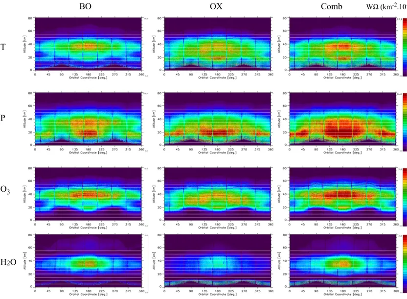
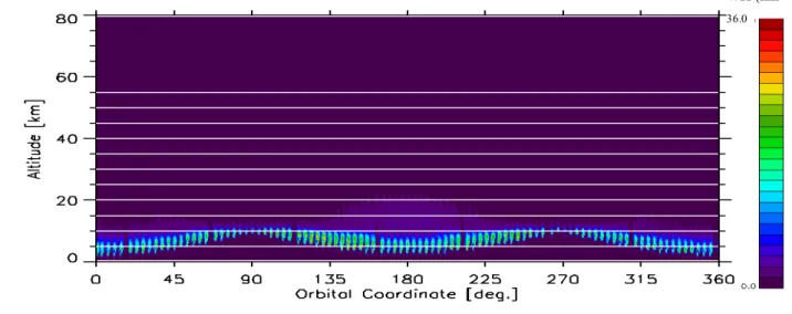
For the analysis of limb-scanning observations with the 2-D approach the atmosphere is partitioned on both the vertical and the horizontal domains [19], [16]. This discretization leads to a web-like picture in which consecutive altitude levels and vertical radii define plane figures denoted as “cloves” (see Fig. 4.1). If the simultaneous analysis of several observation geometries is considered, we can assign to each clove the Information Load (IL) scalar quantifier (Ω) defined as [20]:

(Eq. 4.1) Ω (q,h) = IL of clove h with respect to atmospheric parameter q.

(28)

l = number of observation geometries that go through clove h, m = number of MWs in observation geometry i,

n = number of spectral points in MW j.

Eq. (4.1) can be written as:

(Eq. 4.2) where k is a vector containing the derivatives of all the observations that depend on the value of q in clove h. If the observations are affected by different noise levels (e.g. occur in different spectral bands) it is suitable to use the weighted IL (WΩ) defined as:

(Eq. 4.3) where S is the variance-covariance matrix of the observations relative to all the spectral points that contribute to the information load in clove h.

The uncertainty on the value of the target quantity q in clove h is connected with the quantity 1/WΩ (see [20]).

A map of the WΩ quantifier, calculated for each clove of the 2-D atmospheric discretization permits to evaluate the distribution of the information load with respect to the geophysical parameter q. In these maps:

● The values of WΩ measure the amount of information contained in the corresponding cloves.

● The spatial distribution of WΩ indicates the regions of the atmosphere where the information is gathered from when operating a retrieval analysis.

The IL analysis provides a tool to compare the performance of different observation strategies and/or of different sets of spectral intervals. The WΩ maps also indicate the optimal strategy to select the geo-location of the retrieval grid.

In the 2-D context the observation geometries that look at clove h may come from different limb-scans while in the 1-D context they are a subset of the observation geometries of the analysed limb-scan.

The IL will be computed thanks to the software called “GMTR_INFO”, derived from the GMTR software (Chap. 3)

(29)

4.3 Systematic and Random errors

The measurement are affected by errors that can be divided into two types of errors, indeed the total error is the square summation of the random and systematic errors. The random error is due to the propagation of instrument noise through the retrieval. Random errors are inconsistent with the repetition of measurement, they are scattered about the true value and tend to lack arithmetic meaning. Random errors are caused by unpredictable fluctuations due to interference of the environment with the measurement process.

The MW selection algorithm provide an estimate of the systematic error, which is the root sum square of individual systematic error sources:

• Non Local Thermodynamic Equilibrium (NLTE) error is due to assumption of local thermodynamic equilibrium when modelling emission in the MIPAS forward model. Based on calculations using vibrational temperatures supplied by M.Lopez-Puertas, IAA, Granada.

• Spectroscopic Database Errors (SPECDB formerly referred to as HITRAN) is due to uncertainties in the strength, position and width of infrared emission lines. Based on estimates supplied for each molecule/band by J.M.Flaud, LPM, Paris.

• Radiometric Gain Uncertainty (GAIN) is due mostly to non-linearity correction in bands of the recorded spectra.

• The SPREAD is the uncertainty in width of apodised instrument line shape (AILS). A value of 0.2% has been assumed based on likely variations in apodised instrument line shape from modelled.

• The SHIFT is the uncertainty in the spectral calibration. The design specification of

±0.001cm-1 has been used, and is consistent with the 1st derivatives signatures in the

residual spectra.

• CO2 line-mixing (CO2MIX) is due to neglecting line-mixing effects in the retrieval forward model (only affects strong CO2 Q branches in the MIPAS spectral bands).

• The CTMERR is the uncertainty in gaseous continua. Assumes an uncertainty of ±25% in the modelling of continuum features of H2O (mostly), CO2, O2 and N2.

• Horizontal gradient effects (GRA) is due to the assumption in the retrieval process of a horizontally homogeneous atmosphere for each profile. Error is calculated assuming a ± 1K/100km horizontal temperature gradient.

• Uncertainty in high-altitude column (HIALT) is due to the assumption in the Retrieval process of a fixed-shape of atmospheric profile above the top retrieval level. Effect is calculated assuming `true' profile can deviate by climatological variability.

• The propagation of Pressure and Temperature (PT) random covariance into VMR retrieval.

(30)

• The uncertainties in assumed profiles (profiles supplied by J.Remedios, U.Leicester) of contaminant species (i.e. CH4, H2O, HNO3, N2O, NO2, O3) [species]. For most species this is the climatological 1-σ variability.

The definition of 'systematic error' here includes everything which is not propagation of the random instrument noise through the retrieval. However, to use these errors in a statistically correct manner for comparisons with other measurements is not straightforward. Each systematic error has its own length/time scale: on shorter scales it contributes to the Bias and on longer scales contributes to the Standard Deviation (SD) of the comparison.

Fortunately, two of the larger systematic errors (PT and SPECDB) can be treated properly:

• The propagation error (PT) is uncorrelated between any two MIPAS profiles (since it is just the propagation of the random component of the PT retrieval error through the VMR retrieval) so contributes to the SD of any profile comparison.

• Spectroscopic database errors (SPECDB) are constant but of unknown sign, so will always contribute to the Bias of any comparison, but note that the magnitude of these errors is very uncertain.

Of the other significant errors, the calibration-related errors (GAIN, SHIFT, SPREAD) should, in principle, be uncorrelated between calibration cycles however analysis of the residuals suggests that these errors are almost constant so could be included in the Bias.

The high altitude column (HIALT) and contaminant gas errors ([species]) are likely to be correlated over small areas (1000km) or times (weeks), hence contribute to the Bias for localised comparisons, but as the comparison datasets are extended these errors will contribute more to the SD.

Line mixing errors (CO2MIX) are also contribute towards the Bias but in principle the sign of these errors is known (unlike spectroscopic errors) so this bias could be removed. NLTE errors should also, in principle, contribute a known Bias but these are highly variable (especially diurnally) so care has to be taken to make sure that representative conditions for the comparison are used. [21]

(31)

Performance

of the

(32)

5 Comparison of the two sets of Micro-Windows

using retrievals on simulated observations

The MIPAS instrument is recording spectra which are then used to retrieve the altitude distribution of different targets (Chap 1). This duty is achieved thanks to the GMTR software (Geofit Multi-Target Retrieval), described in Chap. 3. To avoid the redundancy of information and the interference between species the GMTR software extracts, from the spectra, narrow spectral intervals, called Micro-Windows (MWs) (see Sub-Sect. 3.2.1). The Oxford University and the University of Bologna have provided different sets of MWs. The aim of this chapter is to compare the efficiency of these two sets of MWs. I am comparing the two sets of MWs using retrieval on simulated observations, in order to compare the retrieved profiles w.r.t. the reference profiles (Sect. 4.1).

The orbits 31277 and 31278 of February, 23th 2008 are used to calculate the simulated observations in chapters 5 and 7 and to compute the IL values in chapter 6.

5.1 Comparison of the simulated retrievals

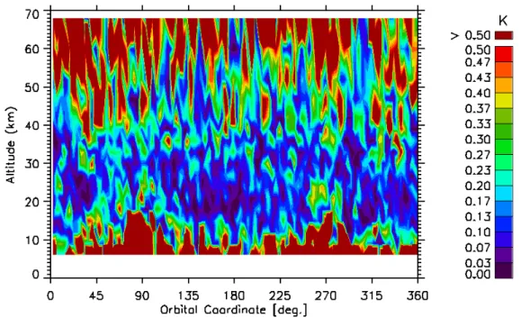
As described in Sub-Sect. 3.3.3 the GMTR software can be use to generate simulated retrievals. In order to compare the retrieved profiles from Oxford University (OX) and Bologna University (BO) sets of MWs, I used the MAPPA tool to convert the profiles over the full orbit into maps. MAPPA is a graphical software written in IDL language which plots all the retrieved profiles corresponding to one species into a single map, as a function of altitude and Orbital Coordinate (OC), that is the angular coordinate θ originating at the North pole and spanning the orbit plane over its 360° extension.

The values plotted on the maps are calculated using three equations:

(5.1)

(5.2)

(5.3)

where “ret” corresponds to the profiles retrieved from the OX and the Bo sets of MWs, “ref” corresponds to the reference profiles and “esd” corresponds to the values of the Estimated Standard Deviation (ESD), as provided by GMTR. The purpose of these quantifiers will be described in Sect. 5.2.1. In Figs. 5.1 and 5.2 are plotted DIFF values for Temperature as a function of altitude and OC for OX and Bo sets of MWs respectively. In Figs. 5.1 and 5.2 I can localise very precisely where the divergence occurs between the retrievals from BO and OX sets of MWs. But to compare the performance of the two sets of MWs it is preferable to have an overall picture of the divergence between the retrievals. In Sect. 5.2, I describe the employed strategy.

DIFF =∣ret −ref ∣

Ratio_ref=∣ret−ref ∣/ref

(33)

Figure 5.1: DIFF values for Temperature as a function of altitude and OC for the OX set of MWs

(34)

5.2 Comparison of the simulated retrievals using

Quantifiers

To facilitate the comparison of the retrievals, I will introduce in sub-section 5.2.1, several quantifiers which refer to a single profile obtained with a full coverage orbit average.

5.2.1 Quantifiers Descriptions

a) AVE[DIFF] is the average value over the full orbit, at each altitude, of the absolute difference between retrieved and reference profile :

(Eq. 5.4)

where N represents the number of values over the full orbit at one given altitude. AVE[DIFF] represents the average difference (without sign) between the retrieved values and the reference values. As explained in Sub-Sect. 3.3.3, the reference profiles represent what would be the retrieved profiles in the case of a perfect retrieval process, so AVE[DIFF] represents the “real” error of the retrieval process. On the other hand, the performance of the retrieval process is linked to the selection of the MWs, i.e. a better choice of MWs will lead to a better efficiency of the retrieval process. Therefore comparing the AVE[DIFF] values arising from the two sets of MWs, I can state which of the two sets of MWs is the most efficient.

For each target, the AVE[DIFF] values of the OX and BO sets of MWs will be plotted as a function of altitude, in black and in blue respectively. To abridge the description of these graphs, a divergence between the two curves will be directly connected to a better or a worse retrieval process which is caused by one of the two sets of MWs.

b) AVE[Ratioref] is the percentage of AVE[DIFF] w.r.t. the retrieved profile:

(Eq. 5.5)

AVE[Ratioref] indicates the magnitude of the average difference w.r.t. the magnitude of

the reference profiles (e.g. if the average difference is high w.r.t. the magnitude of the reference values, the result of this equation will be significantly high). Plotted values on the AVE[DIFF] graphs will be respectively revealed or hidden depending on their

AVE [ Ratio_ref]=

∑

i=1 N

∣reti−refi∣/refi

N ×100 AVE [ DIFF ]=

∑

i=1 N ∣ret_i−ref_i∣ N

(35)

relevance.

For each target, the AVE[Ratioref] values of the OX and BO sets of MWs will be plotted

as a function of altitude, in black and in blue respectively. This quantifier will help us to judge the improvement or worsening magnitude (slight, intermediate or large).

c) AVE[Ratioesd] is the average of DIFF divided by the values of the ESD:

(Eq. 5.6)

AVE[Ratioesd] indicates the magnitude of the average difference w.r.t. the magnitude of

the ESD. The ESD represents the estimated random error of the retrieved values. If this ratio is lower than three, i.e. the average difference is not three times greater than the ESD, then ESD and AVE[DIFF] are considered consistent. Moreover, the difference represent the real error therefore the closer the average value of the oscillations of this quantifier is to one, the better the ESD is reliable.

For each target, the AVE[Ratioesd] values of the OX and BO sets of MWs will be plotted

as a function of altitude, in black and in blue respectively. To abridge the description of these graphs, I will directly link an average value of the AVE[Ratioesd] oscillations nearer to

one to a better consistency between the real and estimated error of one of the two sets of MWs.

d) AVE[ESD] is the average of ESD:

AVE [ ESD ]=

∑

i=1 N esd_i N (Eq. 5.7)

AVE[ESD] indicates the estimation of the software on the value of the error.

For each target, the AVE[ESD] values of the OX and BO sets of MWs will be plotted as a function of altitude, in black and in blue respectively.

As described in Sub-Sects. 3.3.1 and 3.2.2, I used the “cascade” mode to retrieve first the four mains targets simultaneously: Temperature, Pressure, Ozone and Water and then Nitric Acid, Methane, Nitrous Oxide and Nitrogen Dioxide. The magnitude of the peaks on the recorded spectrum will depend of the excitation of the molecules, therefore the results of the four last targets is dependant of the result of the mains targets (mainly temperature). Although the tested MWs only concern the retrieval of the four mains targets, I will also report the plotted quantifiers of the four others species in order to identify some eventual side-effects.

In order to compare the efficiency of the two sets of MWs, I present from Sub-Sects 5.2.2 to 5.2.9 the plotted quantifiers of the set of MW provided by Oxford University (OX) and the set of MWs provided by the University of Bologna (BO) as a function of altitude on the same Figure.

AVE [ Ratio_esd]=

∑