Scuola di Dottorato in Ingegneria "Leonardo da Vinci"
Corso di Dottorato di Ricerca in
TELERILEVAMENTO
Tesi di Dottorato di Ricerca
Adaptive waveform algorithms for HF-OTH skywave radar
Autore:
Relatore:
Anna Lisa Saverino
Prof. Enzo Dalle Mese
__________
__________
Ing. Marco Martorella
__________
Prof. Fabrizio Berizzi
__________
2008 - 2010 SSD ING-INF/03
Abstract
Since 1960, Over the Horizon radars have been studied; they fall into two types: Sky-wave and Surface-wave radar systems, classified as a function of electromagnetic waves propaga-tion mode. The HF-OTH skywave performance strongly depends on several space-time variant factors such as, propagation channel, external noise (environment and man-made noise) and fre-quencies national plan usage. This implies that a HF system must have a high level of adaptively in order to fit the external constrains. This thesis is concerned with a software-defined frequency management system whose main task is to select the transmitted frequencies and elevation an-gles to be used in transmission according to the ionosphere channel, external noise intensity and available channels; special attention was paid to the study of waveforms and specifically to development of a technique for set the waveform parameters in an adaptive way depending on the operating modes.
Contents
Abstract iii
1 Introduction 1
2 HF-OTH Radar 3
2.1 HF-OTH Skywave overview . . . 3
2.1.1 Relocatable Over-the-Horizon Radar (ROTHR) . . . 3
2.1.2 Jindalee Operational Radar Network (JORN) . . . 5
2.1.3 NOSTRADAMUS Radar (New Transhorizon Decametric System Ap-plying Studio Methods) . . . 7
2.2 Differences between HF and Microwave radar . . . 7
3 Ionosphere Channel Characterization 12 3.1 The Ionosphere . . . 12
3.2 Ionosphere propagation channel parameters . . . 16
3.3 Propagation Models . . . 21
4 Frequency Management 24 4.1 Radar System Architecture . . . 25
4.2 FMS Architecture . . . 27
4.3 Available Channels Analysis . . . 29
4.4 Ionosphere Data Analysis . . . 32
4.5 The Parameters Selection System . . . 36
4.5.1 The Antenna Elevation Angle System . . . 37
5 Adaptive Waveform Algorithms 46
5.1 Transmitted Waveform Model . . . 47
5.1.1 Pulsed Waveform Instantaneous Multifrequency (IM) . . . 47
5.1.2 Pulsed Waveform SeQuential Multifrequency (SQM) . . . 49
5.2 Pulse Compression by Encoding . . . 50
5.3 Waveform Parameters Setting . . . 57
5.3.1 Signal Bandwidth selection . . . 59
5.3.2 Duration and Pulse Repetition Time: First Level Adaptivity . . . 60
5.3.3 Duration and Pulse Repetition Time: Second Level Adaptivity . . . 65
6 Numerical Results 66 6.1 R1 - Full Area Surveillance . . . 67
6.1.1 First Radar Scenario . . . 67
6.1.2 Frequency Management System . . . 68
6.1.2.1 Available Channels Identification . . . 68
6.1.2.2 IPC System - Ionosphere Data Analysis . . . 72
6.1.2.3 Elevation Antenna Angle System . . . 74
6.1.2.4 Scanning Frequency System and Transmitted Frequency Se-lection . . . 76
6.1.3 Second Radar Scenario . . . 77
6.1.4 Waveform Selection System . . . 79
6.2 R3 - Small Area Surveillance . . . 81
7 Conclusions 84
List of Tables
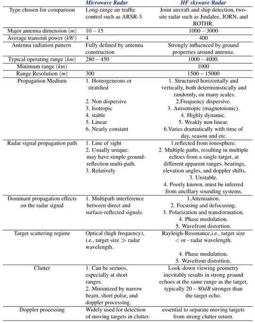
2.1 Key differences between OTH Skywave radar and microwave radar (part 1) . . 10
2.2 Key differences between OTH Skywave radar and microwave radar (part 2) . . 11
4.1 c and d values . . . 31
4.2 Output Table Template for a given azimuth ϑ . . . 45
5.1 Characteristic Parameters of the Waveforms in Radar Systems in use . . . 47
6.1 Numerical Data of Radar Scenario . . . 68
6.2 Table of the Available Frequencies according to NFAP . . . 69
6.3 Removed Frequencies according to Available Band . . . 70
6.4 Removed Frequencies according to Noisy Channels . . . 71
6.5 Available Channels . . . 71
6.6 FMS output table template for a given azimuth ϑ = 135◦ . . . 77
6.7 Reduced OFT - second scenario . . . 79
List of Figures
2.1 ROTHR Transmitter . . . 4
2.2 ROTHR Receiver . . . 4
2.3 ROTHRs Coverage Area . . . 5
2.4 JORNs Coverage Area . . . 6
2.5 Transmitting and Receiving antenna array of Laverton . . . 6
2.6 Nostradamus System . . . 8
3.1 Layers of Earth surface . . . 13
3.2 Free electron production . . . 13
3.3 Loss of Free electron in the Ionosphere . . . 14
3.4 Morphology of Ionosphere . . . 15
3.5 Ionospheric Layers (Day and Night) . . . 16
3.6 Refraction in a stratiform medium . . . 17
3.7 Range of usable frequencies . . . 19
3.8 Propagation paths for fixed elevation angle . . . 20
3.9 Propagation paths for fixed frequency . . . 20
3.10 Simplified geometry representing actual (solid line) and virtual (dashed line) path . . . 21
3.11 Example of ionogram [15] . . . 22
4.1 System Architecture . . . 25
4.2 Waveform Generation System . . . 26
4.3 FMS Architecture . . . 28
4.4 Artificial Noise Power per Hertz . . . 31
4.7 Example of a single ray path . . . 33
4.8 Theoretical Example of a single IPC in ground range . . . 34
4.9 Theoretical Example of IPC in ground range and MTF value for a given eleva-tion angle . . . 35
4.10 Theoretical Example of set of antenna elevation angle and related curves of Rmgr, RMgr 39 4.11 Example of a single footprint . . . 39
4.12 Example of iso-MTF cells . . . 41
4.13 Example of Scanning Frequency Computation . . . 41
4.14 Example of frequency - elevation pairs for each iso-MTF cell . . . 42
4.15 NRCS for horizontal polarization . . . 44
4.16 NRCS for vertical polarization . . . 44
4.17 Sea NRCS plot . . . 45
5.1 Waveform Generation System . . . 46
5.2 Pulse-Code Instantaneous Waveform . . . 49
5.3 Pulse-Code Sequential Waveform . . . 50
5.4 Normalized Ambiguity Function of L-FM pulse with D = 15 . . . 52
5.5 Normalized Ambiguity Function of C-FM pulse with D = 15 . . . 53
5.6 Normalized Ambiguity Function of V-FM pulse with D = 15 . . . 53
5.7 Normalized Ambiguity Function of QUAD-FM pulse with D = 15 . . . 54
5.8 Normalized Ambiguity Function of Frank code of length 16 . . . 55
5.9 Normalized Ambiguity Function of P4 code of length 16 . . . 55
5.10 Mismatch Losses due to linear distortion of amplitude and phase, with β = 0.1 as a function of ∆Φrmsfor quadratic (blu lines) and cubic (red lines) ∆Φ( f ), for L-FM, C-FM, QUAD-FM e V-FM modulations . . . 56
5.11 Surveillance Area . . . 61
5.12 Antenna Footprint for the frequency and elevation pairs related to OFT . . . 61
5.13 Technique of Calculation of both Ground Range and Group Delay . . . 61
5.14 Unambiguous Condition . . . 62
6.1 Radar Scenario . . . 67
6.2 FMS Architecture . . . 69
6.3 Simulated Electron Density Profile . . . 72
6.4 IPC in ground range {SSN = 150, Month = April, Hour = 18} . . . 73
6.5 IPC in ground range {SSN = 50, Month = January, Hour = 2} . . . 74
6.6 Set of antenna elevation angles and related curves of Rgr,m(βj, fi), RgrM(βj, fi) (ref. Figure 6.4) . . . 75
6.7 Set of antenna elevation angles and related curves of Rgr,m(βj, fi), RgrM(βj, fi) (ref. Figure 6.5) . . . 75
6.8 iso-MTF cells (ref. Figure 6.4) . . . 76
6.9 IPC system output - second scenario . . . 78
6.10 Elevation Antenna Angle system output - second scenario . . . 78
6.11 iso-MTF cells - second scenario . . . 78
6.12 Minimum Group Delay (ref. Table 6.7 . . . 80
6.13 Maximum Group Delay (ref. Table 6.7 . . . 80
6.14 PRF as function of elevation angle . . . 81
6.15 Minimum Group Delay versus ionospheric conditions . . . 82
6.16 Maximum Group Delay versus ionospheric conditions . . . 83
Chapter 1
Introduction
Radar ( radio detection and ranging), is a sensor that uses radio waves to detect targets such as aircraft, ships and so on. The radio waves propagation’s mode depends on the used frequencies range; specifically at microwaves employed by conventional radars, the radio waves travel in a straight line and this generally limits their horizon due to the curvature of the Earth.
This restriction was surpassed by means of radars operating in the HF (3 to 30MHz) band thanks to ability of the ionosphere to reflect radar transmitted signals (skywave radars).
In the HF band, there is another wave propagation mode that exploits the ability of signals to propagate by means diffraction over the sea, independently of the atmosphere and ionosphere above it (surface wave radars) [1]. These two radars’ categories are different not only in the way the electromagnetic wave travels beyond the optical horizon but also for their maximum ranges, which are up to not more than 400km in the surface wave radar. This thesis focuses on skywave radar, namely Over The Horizon (OTH) radar, for the reasons mentioned above.
The concept of Over The Horizon (OTH) radar was introduced in the 1950s and 60s by ex-URSS for military purposes in order to detect targets at very long distances, typically up to thousands of kilometers away from the radar. The technological progress (computational ability of modern computers and remarkable development in the digital progressing) has enabled the design of sophisticated systems both in terms of maximum range and in terms of the resolution and accuracy achieved. Nowadays, these radars continue to be used not only for military reasons but also for air traffic control, monitoring of climate change, forecast of hurricanes and so on. Moreover, these systems, which are certainly of strong environmental impact because of their
big size, are installed in several countries (USA, Russia, Australia, France and China) and are managed mainly by military authorities.
Though the OTH radar functioning is very simply, its implementation presents some draw-backs due principally to space-time variations of ionospheric channel, strong presence of exter-nal noise (atmospheric, cosmic and man-made) as well as the congestion of HF bandwidth, that restricts the set of available frequencies. This implies that an HF system must have a high level of adaptively in order to fit the external constrains.
To this purpose, a suitable Frequency Management System (FMS) is needed, able to provide the real time frequency allocation map relative to the surveillance area, according to the ionosphere propagation conditions as well as the background noise scenario.
Chapter 2
HF-OTH Radar
2.1
HF-OTH Skywave overview
Before analyzing the functionalities of HF-OTH skywave systems, a their overview is following summarized; for each system the main features will be highlighted in order to make a compar-ison with results related to our studies. The systems described below are the U.S. ROTHR, the Australian JORN and the French Nostradamus.
2.1.1
Relocatable Over-the-Horizon Radar (ROTHR)
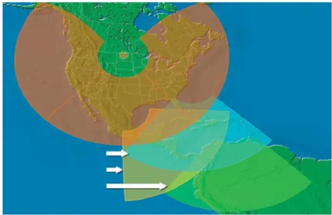
The Relocatable Over-the-Horizon Radar (ROTHR) [2]-[3] designed for Fleet Surveillance Sup-port Command (FSSC) U.S. Navy, is a quasi-monostatic radar that reliably detects aircrafts and ships within a surveillance area of up 300miles inland and 2000miles off the U.S. coast line. The main missions of this system are of homeland security and of counter drug in the Caribbean sea and South America.
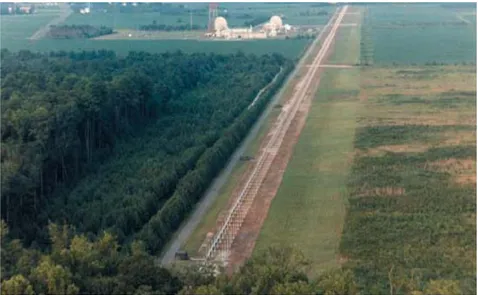
It is based on three sites: Transmitter (Figure 2.1), Receiver (Figure 2.2) and Operational Con-trol Center (OCC) which may be co-located with the receiving Site. The Receive and Transmit sites are separated by a distance of at least 40miles to ensure non interference of radar oper-ations while processing and analysis occurs at the OCC in order to extract target information. The operational head office are in Virginia, Texas and Puerto Rico (Figure 2.3).
The system is supplemented with a network of ionosondes that measures the ionosphere height at mid-range of the designed coverage area and collected data are employed to build an
Figure 2.1: ROTHR Transmitter
Figure 2.2: ROTHR Receiver
area grid. This system makes use of 16 log-Periodic antennas to transmit the Linear FM/CW and 372 receiver channels to pick up energy portion backscattered by target; the azimuth and elevation angle are selected by the management of a phased array, while the frequency and ionosphere height determine the reached range within the coverage area. To select the waveform, the ROTHR must choose properly the following characteristic parameters:
Figure 2.3: ROTHRs Coverage Area
1. Repetition Rate Waveform (WRF) values between 5Hz and 60Hz; 2. Operating frequency between 5MHZ and 28MHz;
3. Bandwidth per sweep, typically between 4.17 and 100 kHz.
2.1.2
Jindalee Operational Radar Network (JORN)
For several years the Australian Defense Science and Technology Organization (DSTO) had invested in the study of HF-OTH skywave radar systems, finally between 1972 and 1974 a pro-totype was developed under so-called Jindalee project [4]-[5]. In the initial stage of the project, the system conceived as bistatic radar consisted of a transmitter located at Harts Range and a receiver located 160km away from Alice Springs. After several stages of improvements brought to Alice Springs site, two new sites became operational, specifically the Laverton (Western Aus-tralia) and Longreach (Queensland) sites. Nowadays, the Alice Springs site is only used for scientific purposes while the other two systems form the so-called Jindalee Operational Radar Network (JORN). More precisely, the Laverton site consists of two bistatic radar systems and provides coverage over a sector angle of about 180degrees, while a third system still bistatic, is located in Longreach with coverage of 90degrees (Figure 2.4).
Figure 2.4: JORNs Coverage Area
The Longreach and Laverton sites are composed by 28 solid-state amplifiers for a maximum transmitted power of 300kW . The transmitted antenna of Laverton showed in Figure 2.5
Figure 2.5: Transmitting and Receiving antenna array of Laverton
is a linear array which 8-16 vertical log-periodic elements, each of which drove by a FM/CW synthesizer [6]. The carrier ranges between 5 − 32MHz while the bandwidth varies from 4-40KHz. The receiving antennas array which extends over an area of 3km for 300km, consists of
480 radiating elements. the functionalities of whole system are supported by eleven cooperating ionosondes.
The innovative concept linked to this project is the integration between sensors in order to form a network of radar: the function of transmission, reception and synchronization will be performed by the three units mentioned above and the signal processing will be carried out remotely from the JORN Control Centre, located in Adelaide in South Australia [7].
2.1.3
NOSTRADAMUS Radar (New Transhorizon Decametric System
Applying Studio Methods)
The Nostradamus radar, located about 160km off Paris, was designed in the 1984 by ONERA with the support of the French Ministry of Defense [8]-[9]. It is a monostatic pulses radar which consists of a planar array with 800m diameter and having a star structure with 288 biconical an-tenna elements subdivided into 19 sub-array randomly distributed over three arms (Figure 2.6); the elements biconical design allows beam elevation control while their random distribution was studied in order to reduce the mutual coupling and the grating lobes.
This innovative configuration allows a 360◦coverage in azimuth.
2.2
Differences between HF and Microwave radar
From above remarks radar operating in the HF band (3MHz − 30MHz) can be classified accord-ing to propagation mechanism of electromagnetic (e.m.) waves, which may be or via skywave as ROTHR [2]-[3], Jindalee [4]-[5] and Nostradamus [8]-[9] system, or via surface wave as SECAR [10] and the others. Specifically Over The Horizon (OTH) skywave radar [1] allows covering wide area surveillance from about 500 − 600km up to 3000 − 3500km, thanks to iono-sphere electromagnetic reflection.
Below the operating principle is summarized; the transmitted signal is reflected by the ionospheric layers and hits targets over the horizon; the same path is followed by target echo travelling toward the radar from which it is then exploited in Doppler domain to distinguish the moving targets from land and/or sea Clutter.
Figure 2.6: Nostradamus System
To understand the benefits and at the same time the problems related to design of HF-OTH skywave radar, are highlighted below its main features with respect to classical microwave radar [1]:
1. Transmitted frequencies must belong to band between 3MHz and 30MHz according with ionospheric propagation channel;
2. Long radar coverage is allowed up to 4000km corresponding to a zero antenna elevation angle. In practical applications it is convenient to limit the maximum distance to about 3000km to avoid low antenna elevation angle as well as layer ionosphere internal multi-path;
3. Blind area for distances less than about 400 − 600km exists; indeed when the e.m. wave strikes the ionosphere with an incidence angle greater than a critical value, the transmitted signal is not reflected and no returns occur;
4. The ionospheric channel is space-time variant. The propagation behaviour is dependent on the transmitted frequency, date, solar activity identified by Sun Spot Number (SSN) and radar geographical coordinates (TxLat, TxLon);
5. In the HF band, radar performances are heavily affected by background noise, which is mainly due to atmospheric, cosmic and man-made noise.
Internal noise caused by thermal effect is almost negligible;
6. We must deal with heavy propagation losses due to very long travelling distances as well as strong absorption losses caused by ionospheric dispersion. The whole loss contribution can be up to 100 − 150dB;
7. The HF spectrum is heavy crowded by communications and broadcasting traffic, which often restricts the bandwidth available for radar operation. Therefore, free channels are limited and often available within a limited time interval;
8. The antenna system requirements are particularly demanding because of wide operating band;
9. High values of peak power are necessary in such systems to contrast the strong losses; 10. HF radar cross section (RCS) of targets is regulated by different mechanism than in
mi-crowave regions;
11. The principle of operation for an HF-OTH skywave radar shows a spatial resolution cell that is range dependent;
12. HF-OTH radar is strongly multifunction; it can operate in different modes aiming to dif-ferent tasks. Typical missions are target detection on a limited surveillance area, detection of specific type of targets (e.g.: ships), coordinate registration, sea surface monitoring, others (Table 2.1)-(Table 2.2).
So the factors which influencing skywave radar performance are:
1. The environmental impact produced from the greater dimension of antennas array which is proportional to employed wavelength;
Microwave Radar HF skywave Radar
Frequency Constraints Can be serious 1. Bounded above by the statistical because of the needed for availability of skywave propagation wideband radar systems to ranges of interest. and by competition 2. Bounded below by spectrum for the microwave availability, antenna size, and the frequency spectrum by rapid fall-off in target RCS communications and other 3. Must not interfere with other users electromagnetic services in the crowded HF spectrum,thus
limiting choice of frequency and bandwidth.
4. Must adapt continually to the changing ionosphere so as to maintain illumination of current
target region. Noise floor dominated by Internal receiver noise sources (atmospheric, galactic,
(thermal, etc) anthropogenic, etc.) Siting Constraints Unobstructed, elevated 1. receive array site must be EM
sites preferred quiet, generally rural, to avoid city and industrial noise at HF
frequencies. 2. Huge arrays require flat,open spaces to minimize topographic
effect on beam patterns. 3. If a bistatic or two-site
quasi-monostatic design is adopted, it needs (two sites with adequate separation (˜100km) and the correct geographical relationship
relative to the coverage area. 4. Location on the Earth must be such
that auroral and equatorial spread doppler echoes don’t mask targets.
Table 2.1: Key differences between OTH Skywave radar and microwave radar (part 1)
2. High clutter return because of wide illuminated area; 3. HF band occupancy;
4. Strong space-time variations of propagation channel.
All these factors are dependent on transmitted frequency, hence the frequency choose is one of the main critical aspects of whole system design, furthermore under certain conditions it allows to reach a given point rather than another. Therefore it is evident that an HF radar must be an adaptive system where transmitted waveforms, antenna system as well as signal processing, must be tuned according to external constrains; dedicated sub-systems are needed in order to collect environmental information.
Microwave Radar HF skywave Radar
Type chosen for comparison Long-range air traffic Joint aircraft and ship detection, two-control such as ARSR-3 site radar such as Jindalee, JORN, and
ROTHR. Major antenna dimension (m) 10 − 15 1000 − 3000 Average transmit power (kW ) 4 400
Antenna radiation pattern Fully defined by antenna Strongly influenced by ground construction properties around antenna. Typical operating range (km) 280 − 450 1000 − 4000.
Minimum range (km) 1000 Range Resolution (m) 300 1500 − 15000
Propagation Medium 1. Homogeneous or 1. Structured horizontally and stratified vertically, both deterministically and
randomly, on many scales. 2. Non dispersive 2.Frequency dispersive. 3. Isotropic 3. Anisotropic (magnetoionic). 4. stable 4. Highly dynamic. 5. Linear 5. Weakly non linear. 6. Nearly constant 6.Varies dramatically with time of
day, season and etc. Radar signal propagation path 1. Line of sight 1.reflected from ionosphere.
2. Usually unique; 2. Multiple paths, resulting in multiple may have simple ground- echoes from a single target, at reflection multi-path. different apparent ranges, bearings, 3. Relatively elevation angles, and doppler shifts.
3. Unstable.
4. Poorly known, must be inferred from ancillary sounding systems. Dominant propagation effects 1. Multipath interference 1.Attenuation.
on the radar signal between direct and 2. Focusing and defocusing. surface-reflected signals. 3. Polarization and transformation.
4. Phase modulation. 5. Wavefront distortion. Target scattering regime Optical (high frequency), Rayleigh-Resonance,i.e., target size
i.e., target size radar < or - radar wavelength. wavelength.
4. Phase modulation. 5. Wavefront distortion. Clutter 1. Can be seriuos, Look-down viewing geometry
especially at short inevitably results in strong ground ranges. echoes at the same range as the target, 2. Minimized by narrow typically 20 − 80dB stronger than beam, short pulse, and the target echo. doppler processing.
Doppler processing Widely used for detection essential to separate moving targets of moving targets in clutter. from strong clutter return.
Chapter 3
Ionosphere Channel Characterization
HF-OTH radar using skywave propagation via ionospheric refraction is capable of detect targets at distances greater than conventional microwave radar limited by the line of sight. Nevertheless there are some drawbacks operating at these frequencies indeed in certain conditions the signals propagation suffers from many adverse effects such as [11]:
1. Radio energy absorption due to electron-neutral collisions;
2. Multipath caused by presence of more than one propagation path between the transmitter and receiver;
3. Wide fluctuations due to dynamic behaviour of ionosphere.
Therefore a basic study of ionosphere properties is paramount to understanding HF radio propagation over distance. This section is devoted to providing a simplified overview for some of important ionosphere propagation mechanisms as well as discussing limitations due to its complex dynamics.
3.1
The Ionosphere
The ionosphere located in the region at 50 − 500km in altitude above the Earth surface (Fig-ure 3.1) is a broad layer of ionized gas called plasma where charges, either positive or negative, are present in required amount to influence the trajectory of radio waves [11]- [12]. The exis-tence of them results from the components ionization of the neutral atmosphere by means solar
rays and therefore from a photoelectric effect. This phenomenon was experimentally demon-strate around 1925 by different physicists like Aplleton, Barret, Breit, Tuve and Marconi.
Figure 3.1: Layers of Earth surface
Experiments conducted on propagation of radio waves have led us to understand that ioniza-tion is the physical process in which electrons, that are negatively charged, are removed from neutral atoms or molecules to leave positively charged ions and free electrons that have a sensi-tive influence on HF radio waves propagation (Figure 3.2).
Figure 3.2: Free electron production
Loss of free-electrons in the ionosphere occurs when a free electron combines with a charged ion to form a neutral particle (Figure 3.3). Loss of electrons occurs continually, both day and night.
Figure 3.3: Loss of Free electron in the Ionosphere
Therefore the propagation mechanism depends on the free electrons amount in the iono-sphere that changes with seasons, daily-night cycles and with solar radiation. With increasing of the altitude, the intensity of ionizing UV radiation increases while the density of neutral gas available for ionization decreases; this phenomenon causes an augmentation of electron density and the formation of horizontal layers of ionization generally three sometimes four (Figure 3.4):
1. D region: The D region is the lowest part of ionosphere extending from about 50 − 90km. During quiet conditions this region is present only during daylight hours and it is the main responsible of the absorption of high frequency radio waves.
2. E region: The E region extending from about 90 − 140km, is mainly a diurnal region indeed its free electron density is strongly dependent on solar zenith angle with a daily maximum in correspondence of the maximum elevation and a seasonal maximum in sum-mer. During quiet conditions the E layer may have a residual of ionization at nighttime contrary to what happens with the D layer.
Occasionally within this region an unpredictable natural phenomenon called sporadic E occurs; given its unpredictable nature, numerous correlations and observations have been made. This layer is known to have a diurnal pattern, peak near the solstices and occurs more frequently in latitudes closer to equator; moreover it can have a comparable electron density to the F region. Sometimes a sporadic E layer is transparent and allows most of radio wave to reach the F region and receiver also, however at other times it obscures the F region totally (sporadic E blanketing).
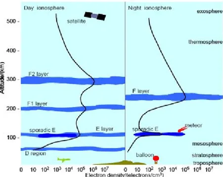
3. F region: The F region, extending from about 140 − 500km above the Earth, is the most prominent layer for HF communications. During the day it split into F1 (140 to 210km)
and F2 (over 210km) sub-layers whereas at night these two layers combine to form a single F layer, usually called F2 layer.
Figure 3.4: Morphology of Ionosphere
It is evident that from a point of view of radio waves propagation between 3MHz and 30MHz, certainly the F2 region has the most significant because:
1. it is present 24 hours of the day;
2. its high altitude allows the longest communication paths; 3. it reflects the highest frequencies in the HF band.
In Figure 3.5 are reported the layers during the day and night.
As it is clear from the above shown, the formation of ionospheric layers is closely related with solar activity that has a periodicity of about eleven years and it is generally evaluated by esti-mating of the average monthly number of sunspots (Sunspot Number - SSN). Other phenomena that influence the refraction mechanism are:
1. Sudden Ionosphere disturbances (SIDs): The SIDs are caused in large part by UV and X-ray generating solar flares. Solar flares occur when sunspots with very complex magnetic fields become unstable and explode. The X-ray and UV energy released by these solar flares makes its way to Earth and interacts with the upper atmosphere to create a SID;
Figure 3.5: Ionospheric Layers (Day and Night)
2. Traveling Ionospheric Disturbances (TIDs).
3.2
Ionosphere propagation channel parameters
The reflective capacity of these layers depends on the gradient of their refractive index (n). Its generic form related to a radio wave which propagates in the ionosphere is very complex [13] and it is known as the Appleton-Hartree equation, however at frequencies above a few MHz it can be simplified to equation 3.1
n= s 1 − f 2 p f2 (3.1) where:
1. n: is the index of refraction; 2. fp: is the plasma frequency;
3. f : is the frequency of radio wave.
When the value in the square root is negative (f ≤ fp) the wave cannot propagate; therefore the
guarantee to be reflected by the ionosphere to earth.
It is correlated to electron density (N) by following expression:
fp= s e2N 4π2m eε0 ≈ 9√N (3.2)
where e is the electron charge, me is its mass and finally the ε0 is the vacuum dielectric
constant. By combining two equations, it follows that the refractive index decreases with raising plasma frequency and thus raising the altitude, so the wave is progressively bended until it is completely deflected towards the ground (Figure 3.6).
Figure 3.6: Refraction in a stratiform medium
The way in which this happens is modeled mathematically by Snell’s law (3.3) :
sin(φ0n0) = sin(φ1n1) = sin(φ2n2) = ... = sin(φmnm) (3.3)
Using the equation 3.3 and applying the secant law we obtain an important relationship between wave frequency and plasma frequency ( 3.4):
f = fpsec φi (3.4)
with φi incident angle; in order to satisfy this equation, it is necessary to select the proper
set of ( f , φi). By looking at the equation (3.4) it is evident that not all frequencies will be
pass straight through the ionosphere whereas if it is too low, the signal energy will be very low due to absorption in the D region. For these reasons when we look at ionospheric propagation, there are several frequencies to be determined to maximize the HF-OTH radar performance. The frequencies include Critical Frequency, Lowest Usable Frequency (LUF), and Maximum Usable Frequency (MUF) [14]:
1. Critical Frequency of the layer-fo: The critical frequency is highest frequency which can
be reflected for normal incidence;
2. Maximum Usable Frequency (MUF): The MUF is defined as highest frequency that guarantees signal propagation over an oblique ionospheric path. Normally we refer to MUF50%, that is the median maximum usable frequency for a given ionospheric path,
month, SSN and hour. In other words it is the frequency for which ionospheric support is predicted on 50% of the days. That means also that sometimes you will only have 1% of chance to work up to this frequency whereas other times 100% of chance but it is im-possible to forecast in what days this will happen. Consequently, the MUF is a random variable and, as such, using the programs of long-term prediction can be estimated mo-ments of various order. Therefore the success of radio link between two points with a frequency of transmission, is characterized by the probability that it is greater than trans-mitted frequency. For these reasons the operating frequency is chosen below the predicted MUF;
3. Lowest Usable Frequency (LUF): The Lowest Usable Frequency is defined as the fre-quency below which the signal falls below minimum strength required for satisfactory reception. It depends on signal-to-noise ratio, power and transmission mode and can also be approximated by 0.65∗MU F.
Therefore from an ionospheric point of view, the LUF and MUF (Figura 3.7) define the max-imum usable spectrum range in which the propagation is open, allowing HF communications and it will vary:
• during the day; • with the seasons;
• with the solar activity, quantified by the Sunspot Number (SSN) index, which represents a monthly average of sunspot numbers;
• from site to site.
Figure 3.7: Range of usable frequencies
Specifically the upper limit of frequencies varies especially with the above factors while the lower limit also depends on receiver site, noise, antenna efficiency, transmitted power and so on. From an operational point of view, starting from physical observations above, it is possible draw the following considerations:
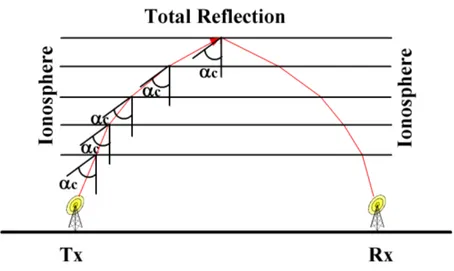
• Fixed Elevation Angle: Greater distances are reached with greater frequencies for a fixed elevation angle (Figure 3.8).
This phenomenon is due to the fact that increasing the frequency value towards the max-imum usable frequency (ray 3 - Figure 3.8), the electromagnetic wave is deflected by the upper layers (ray 1 and ray 2 - Figure 3.8); specifically the maximum reached range is tied to MUF (ray 3 - Figure 3.8) value, beyond which the wave penetrates the ionosphere (ray 4 - Figure 3.8);
Figure 3.8: Propagation paths for fixed elevation angle
• Fixed Frequency: Greater distances are reached with a smaller elevation angle for a fixed frequency, specifically the maximum range is tied to the smaller elevation angle (Figure 3.9).
Figure 3.9: Propagation paths for fixed frequency
It is worth noting that:
1. Increasing the angle, the rays are refracted in layers that are highest in the ionosphere by allowing the reaching of the ground distances that are closer to the radar.
2. The smallest achievable distance is defined as the "Skip Zone" (Figure 3.9); when the ground range distance is equal to the skip zone, the critical angle for that frequency is reached.
To sum up, the ray’s reflection is tied up to the MUF, which depends in turn on both ionospheric conditions and elevation angle. Therefore, elevation angle, frequency and electromagnetic ray
path are strictly correlated variables. In fact, if the frequency is too high the wave will pass through the ionosphere, whether it is too low, the signal energy will be reduced because of D layer absorption.
In particular, it is possible to establish a relationship between a beam that returns to the Earth after being gradually bent by the ionosphere and a ray that propagates in free space and is totally reflected at a given height, known as the "equivalent height" and defined by Breit and Tuve theorem (Figure 3.10).
Figure 3.10: Simplified geometry representing actual (solid line) and virtual (dashed line) path
Summarizing ionospheric features can be described by a set of characteristic parameters so-called "raysets" and identified by:
• Day, month and SSN; • Electron density; • Plasma frequency;
• Virtual height of reflection.
3.3
Propagation Models
The channel modeling is very important to understand how signal path changes with solar ac-tivity; in this regard it is recalled that the most incisive effects on signal propagation are the
amplitude fluctuation (Fading) and phase shift on received echo. These effects are strongly dependent on solar energy, which exhibits significant variability in space and during the day, the season and year. Specifically relevant spatial variations occur across mid-latitude, equato-rial and polar region whereas temporal variations occur diurnally, seasonally and over 11 year solar cycle. Therefore in order to calculate the features of a received radio signal through the ionosphere, such as its amplitude, polarisation, relative phase, time of flight, dispersive spread, it is necessary to know how the variation of electron density influences radio signal path from transmitter to receiver; therefore a monitoring of ionosphere is needed. The most important technique for ionospheric monitoring, makes use of a network of ionosondes which provides all observable parameters for a discrete number of heights and frequencies. An ionospheric sounder is a very simple device that using basic radar techniques, measures the length of time it takes for one reflection, the strength of the reflection, and how high of a frequency can be reflected; from these three data, the ionization density, altitude of ionization and MUF are determined and organized in an ionogram (Figura 3.11).
Figure 3.11: Example of ionogram [15]
Over the years, several models [16] have been developed in order to extract from iono-grams, information about ionospheric behaviour; specifically long term (SWILM [17], SIRM [18], PASHA [19]), short term (IFELMOR [20], ap(t) model [21]) and real time (SIRMUP [22], ISWILM [22]) models have been proposed. Between long-term models the most widely used
is the IRI model which provides a monthly averaged electron density profile, ionospheric tem-perature and ionospheric composition in the altitude range within 50km and 2000km based on reliably measured data with ionosondes. With these parameters, the real position of target can be obtained by using a ray-tracing technique whose main task is to reconstruct, under certain conditions, the real path of electromagnetic wave.
Chapter 4
Frequency Management
The HF-OTH skywave performance strongly depends on several space-time variant factors such as:
• Signal loss due to the dispersion of the propagation medium;
• Formation of multiple beams because of the refraction from different ionospheric layers (the phenomenon of multipath);
• Fluctuation amplitude and phase of the received signal due to the dynamic character of the ionosphere;
• Strong presence of external noise(atmospheric, cosmic and man-made); • Congestion of HF band .
All these factors are highly dependent on the operational frequency, for this reason it is essential to develop a Frequency Management System (FMS) to be used in transmission. The aim is that of providing, the frequency allocation map related to surveillance area from which to derive the waveform parameters, in real time and for each antenna’s azimuth direction. This implies that a HF system must have a high level of adaptively in order to fit the external constrains.
Here we propose a new Frequency Management System [23], whose main task is to provide the operative tables containing the operational elevation angles (β ) with the respective transmission frequencies ( f ) and the waveform parameters:
1. Using the knowledge acquire on: • Ionosphere Channel;
• External noise levels and its spectral distribution;
2. Respecting the restrictions imposed by the National Frequency Allocation Plan (NFAP), that identifies the distribution of spectrum between stake holders, government and non government, as well as providing an indication of the manner in which the radio frequency spectrum is utilized in Italy [24];
3. Taking into account the constraints of the system (eg, antenna, RF amplifier and so on).
4.1
Radar System Architecture
Before analyzing the functionalities developed by the FMS, it is worth introducing briefly,a bigger picture (Figure 4.1). This will help understand what the FMS depends on and what it affords.
The main functionalities are assigned by the Radar Management and Control (RMC), which
Figure 4.1: System Architecture
manages and coordinates each radar sub-system. The Radar Console specifies the radar site, operative mode and surveillance area. These parameters must be set before any other radar functionality. The other main functional blocks are:
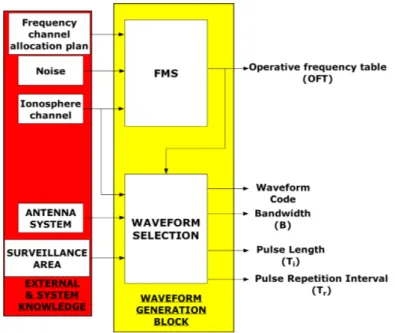
1. The Waveform Generation (WG) block (Figure 4.2), which is composed of the Frequency Management System (FMS) and Waveform Selection System (WSS);
Figure 4.2: Waveform Generation System
the FMS selects the transmitted frequency and antenna elevation angle as a function of the ionospheric channel, external noise level and available clear channels; the WSS selects the other waveform parameters starting from the Operative Frequency Table (OFT), which is an output of FMS containing the transmission frequency map on the surveillance area [5]-[6]. It is worth noting that both FMS and WGS contribute to the real time waveform parameters setting;
2. The Phased antenna array should be controlled in amplitude and phase for each radiating element adaptively as a function of radar operative mode and of the surveillance area; 3. Transceivers are integrated into each single antenna of the array.
Thanks to the low operating frequency (HF band) fully digital architecture can be realized; 4. The Signal Processing, is devoted to targets detection considering the space-time vari-ability of the external scenario (i.e.: external noise and surveillance area) and propagation channel (ionosphere);
5. Data processing is in charge of target tracking.
This is really a complex task in the OTH radar and it needs of suitable algorithms to update the target kinematic parameters and to recalculate the target location;
6. Several modes of data visualization are available for the user, for example the range-Doppler and frequency-angle domain and the synthetic representation.
The definition of the radar parameters (transmitted frequencies and waveform parameters) depends on the radar site, the surveillance area and the available frequencies; all these elements depend on several factors such as antenna system, propagation channel (Ionospheric channel), external noise (environmental and man-made) and National Frequency Allocation Plan (NFAP). Therefore dedicated sub-systems are needed in order to collect environmental information, which will be processed by the frequency selection system for defining the radar parameters. The mentioned sub-systems can be external (Figure 4.1) or integrated into the radar. Specif-ically, a network of ionosondes is used to characterize the ionospheric channel in terms of signal propagation, whereas the external noise level is measured by a HF spectrum analyzer able of providing real time band occupancy; in any case the National Frequency Allocation Plan (NFAP) must be taken into account for every frequency change [24].
All these tasks are performed via software, through suitable algorithms.
The next sections of this chapter will devote to describe the FMS functioning and the algo-rithms that manage it, while the waveform parameters setting with analysis of the same will be argument of next chapter.
4.2
FMS Architecture
Figure 4.3: FMS Architecture
The configuration is composed by: 1. Ionosphere IPC system;
2. Elevation antenna angle system; 3. Scanning frequency system; 4. Transmitted frequencies selection.
The general operation of FMS system, can be subdivided as follows: • Study of available channels;
• Analysis of ionosphere data;
• Finally, selection of radar parameters (azimuth, elevation angle and frequency).
These main functionalities are implemented via software through suitable dedicated algorithms. From a technological point of view, the practical realization of the FMS system can be carried
out by making use of ad hoc computer equipped with DSP or FPGA boards to be easily pro-grammed and reconfigured.
Next sections are devoted to the description of such sub-systems.
4.3
Available Channels Analysis
Before select the frequencies that can be propagate, it is necessary analyze the NFAP and the external noise in order to determine the frequencies set that can be used for the functioning of the skywave radar.
For this purpose the two following blocks are used: • The NFAP Block, this provide the frequencies that:
1. Belong to the HF band;
2. Are reserved to Ministry of Defense;
3. Have the bandwidth that guarantees the required range resolution.
• The External Noise Block, this block determine the noisy channels in order to eliminate them from available frequencies (previous block) and in order to provide the interference - free channels.
In this regard a characterization of the noise must be made.
From above remarks, the external noise is essentially composed by atmospheric, galactic and man-made noise [25] [26].
Atmospheric Noise is radio noise caused by natural atmospheric process, primary light-ing discharges in thunderstorm. It can be observed with a radio receiver in the form of combination of white noise (coming from distant thunderstorms) and impulse noise (coming from a near thunderstorm). The power-sum varies with seasons and nearness of thunderstorm centers.
Although lightning has a broad-spectrum emission, its noise power increases with de-creasing frequency so usually is of a problem in coincidence of a solar minimum and at
night when lower frequencies are needed.
Galactic Noisearises from our galaxy and it will have effects only at the high frequencies.
Man-Made Noise arises from human technologies implanted for power transmission and communications.
The man-made noise that is mainly due to the communication and broadcasting systems, electric energy transport system, automotive ignition, industrial thermal processes and instruments for scientific/medical appliances, is distributed, albeit not uniformly, in all bands.
It are mainly located in business, industrial and residential areas, hence according to degree of industrialization and to population following characterization is used [27]:
1. city: business area with a citizens number more than 200.000 and heavily industrial-ized;
2. residential: residential area with a population is less than 50.000 and little industri-alized;
3. rural: areas characterized by residences that are distributed in an average of over one mile apart and are more than one mile far away from high-voltage power lines; 4. quiet rural: locations that are several kilometers far from any man-made sources.
Equation 4.1 shows the medium noise factor for the artificial noise, according to the data on the external noise provided by Recommendation ITU-R P.372 [26].
Fim= c − d log( f );
Fim= median noise f actor in dB; f = f requency;
(4.1)
c d City 76.8 27.7 Residential 72.5 27.7 Rural 67.2 27.7 Quiet Rural 53.6 28.6
Table 4.1: c and d values
A graphical representation of both artificial and cosmic power noise, is reported respec-tively in Figure 4.4 and Figure 4.5.
Figure 4.5: Cosmic Noise Power per Hertz
4.4
Ionosphere Data Analysis
During this phase, a characterization of ionospheric channel from a radar point of view, it is made. The aim is to determine all the frequencies that can be propagate for a fixed radar sce-nario (radar geographical coordinates, area surveillance and operative mode) and for a fixed ionospheric condition identified by the Sun Spot Numbers (SSN), date and time in order to take full adavantage of the radar. To accomplish this, it is defined a new method in order to synthesize the ionospheric propagation’s conditions from radar point of view.
This method is relied on the ionospheric sounding system and ray-tracing algorithm (Figura 4.6) and it is performed through following steps:
• Ionosphere Data Collection through a network of ionosondes:
During this phase a ionosphere sounding system measures the electron density profiles that are given to Ray-tracing block (Figure 4.6) for the reconstruction of electromagnetic path (Figura 4.7) through the ray-tracing algorithm;
Figure 4.6: Functional Block of ray-tracing algorithm
Figure 4.7: Example of a single ray path
• Ionosphere Data Management and Radar Parameters evaluation by ray-tracing algorithm: Once radar site, date and sun activity (SSN) are known, the Ray-tracing algorithm is ap-plied to the estimated ionosphere electron density spatial distribution (previous step), for radar parameters (group delay, ray-path, ground range distances, Rgr, one way
prop-agation and absorption losses, equivalent height and finally incident angle) evaluation. Specifically for any radar azimuth direction (ϑ ), the ground range point (Rgr) of ray path
intersection on Earth surface is estimated, for a transmitted frequency ( f ) changes within 6 − 30MHz and a fixed elevation angle (β )-(Figure 4.8);
Figure 4.8: Theoretical Example of a single IPC in ground range
• Radar Parameters Collection and Display (IPC System):
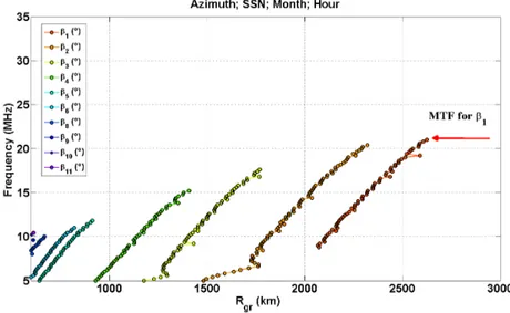
At this point, the above operation is repeated for elevation angles ranges between 6.5◦ and 55◦in order to form an Ionosphere Prediction Chart (Figure 4.9) for a given antenna azimuth angle and for a fixed solar activity.
Therefore the IPC is a family of curves parameterized as a function of elevation angle that provides for any frequency in the HF band, the ground range point of the e.m. ray path of intersection to Earth surface.
The choice of graphics the IPC as a set of iso-elevation curves was dictated mainly by scanning technique in elevation that will be used to illuminate all distances to the ground that belong the surveillance area; this technique will be applied once defined the azimuth angle and the scanning distances will be controlled by adjusting the transmitted frequency. The Figure 4.9 shows an theoretical example of IPC; each color refers to a different elevation angle and the related curve is named iso-elevation curve that is upper bounded by the Maximum Transmitted Frequency (MTF) which is defined as the frequency value 15% lower than the MUF.
The idea of introduce the MTF concept rises from observation that the MUF is strongly de-pendent from solar activity, especially sharp decreasing of MUF due to dynamic phenomena of ionosphere, could cause the absence of ionospheric propagation and consequently the failure of radar operational; moreover it is well known that frequency values near to MUF can generate
Figure 4.9: Theoretical Example of IPC in ground range and MTF value for a given elevation angle
phenomena of ionospheric channeling which cause an anomalous behavior of e.m. ray path and therefore an ambiguity concerning the radar positioning. To sum up the MTF concept is very important in order to guarantee radar operational continuity.
From an operative point of view it is clear (Figure 4.9) that the employment of the IPC alone is problematic because it provides one frequency for each single ground range distances within of surveillance area. Since the number of ground range distances could be theoretically infinite, the number of transmitted frequencies should be infinite too. For this reason in order to reduce the dimensionality of problem, it has been introduced the concept of iso-MTF cell in order to use the same frequency for cover an interval of ground range and azimuth rather than one point.Therefore for a given azimuth angle (ϑ ) and for a fixed ground range point Rgr,
the iso-MTF cell is defined as ground range interval within of which the maximum variation of MTF is less than 10% (equation 4.2)
∆Riso(Rgr) = max d (
|MT F(Rgr) − MT F(Rgr+ d)|
MT F(Rgr)
≤ 0.1) (4.2)
A similar definition it has been introduced for a given ground range and for a fixed azimuth angle (equation 4.3): ∆ϑiso(ϑ (Rgr)) = max α (|MT F(ϑ (Rgr)) − MT F(ϑ (Rgr) + α)| MT F(ϑ (Rgr)) ≤ 0.1) (4.3)
where ϑ is the azimuth angle related to ground range point for which it has been calculated the cell extension.
Then, the iso-MTF cell for a given ground point of coordinates (Rgr,ϑ ) is the ground area of
dimensions ∆Riso(Rgr)∗∆ϑiso(ϑ ) within of which it can be neglect with extreme rationality the
character dynamic of ionosphere.
4.5
The Parameters Selection System
The previous blocks provide the means for determine all frequencies that can be transmitted for an azimuth angle and for a given elevation within 6.5◦ and 55◦, taking into account the ionosphere propagation channel.
Anyway, to maximize the radar performance it is necessary to take into consideration, in ad-dition to the ionosphere, also the functional blocks of the whole system and in particular the antenna system. In fact the return energy is strictly related to the extension of illuminated area which depends on antenna footprint. For this purpose in the last stage, all the information obtained through the above operations are organized according to area surveillance, antenna system, noise level and still according to the ionospheric conditions.
Firstly all the frequency and elevation angle pairs that allow to reach ground range points that not belong the surveillance area, are eliminated.
Then the same zone is partitioned into iso-MTF cells and for any of which , are determined all frequency-elevation couples for which the antenna’s footprint allows to illuminate the same cell.
Finally all these couples are ordered by the maximum radar return and are collected into two tables organized respectively in function of elevation angle and iso-MTF cells; it is last this that is used to evaluated the waveform parameters in adaptive way as a function of illuminated area.
1. Elevation Antenna Angle System; 2. Scanning Frequency System;
3. Transmitted Frequencies Selection System.
The following subsections are devoted to describe any subsystem and especially the algo-rithms that the same subsystems implement.
4.5.1
The Antenna Elevation Angle System
The task of this block is to provide, for a given antenna azimuth ϑ , the set of antenna elevation angles βj, with j= 0,1,2, j(ϑ )-1 that guarantees all ground points to be illuminated by
iono-sphere reflection and taking into account the constrains of antenna system.
The set of antenna elevation angles is calculated in accordance with the following steps: 1. Starting from the higher elevation angle provided from IPC system, the set of elevation
angles {βj(ϑ , f∗)}N( f
∗)
i=1 is determined for each fixed frequency f∗ that belongs to HF
band according to the available channels; the N( f∗) is the number of steering for f∗, that guarantee the coverage continuity.
The continuity is verified when the distance R(i)gr relative to ray path associated to greatest
elevation Rgr(βi(ϑ , f∗) + ∆β (βi(ϑ , f∗), f∗)/2 of antenna beam ∆β (βi(ϑ , f∗), f∗) (Half
Power Beam Width for a fixed βi(ϑ , f∗) and f∗) is less than or equal to the maximum
ground range obtained by the intersection between the Earth surface and the ray-path related to a smaller elevation Rgr(βi−1(ϑ , f∗) − ∆β (βi−1(ϑ , f∗), f∗)/2 (equation 4.4);
βj(ϑ , f∗) ∈ {βj(ϑ , f∗)}N( f ∗) i=1 : { R(i)gr = Rgr(βi(ϑ , f∗) + ∆β (βi(ϑ , f∗), f∗) 2 ) ≤ Rgr(βi−1(ϑ , f∗) − ∆β (βi−1(ϑ , f∗), f∗) 2 ) = R (i−1) gr } (4.4)
Looking at equation 4.4 it is worth underlined that for i = 1, is verified the following initial condition (4.5): β0= 55◦; max(R(0)gr ) = 650km (4.5)
2. Starting from the set above determined, next subset of elevations {βj(ϑ , f )} ¯ N( f )
j=1 ( ¯N( f ) is
the number of steering ), is evaluated in order to have overlap between the ground points reached through the highest elevation angle ( βj(ϑ , f ) + ∆β (βj(ϑ , f ), f )/2 ) into antenna
beam ( ∆β (βj(ϑ , f ), f ) ) and the maximum of smaller distances ( max(Rgrj−1) ) reached
through previous angle (equation 4.6);
βj(ϑ , f ) ∈ {βj(ϑ , f )} ¯ N( f ) j=0 : { R( j)gr = Rgr(βj(ϑ , f ) + ∆β (βj(ϑ , f ), f ) 2 ) ≤ Rgr(βj−1(ϑ , f ) − ∆β (βj−1(ϑ , f ), f ) 2 ) = R ( j−1) gr } (4.6)
3. Starting from the subset {βj(ϑ , f )} ¯ N( f )
j=1 , next elevation angle is determined in order to
guarantee the minimum overlap with the previous elevation; therefore the winning angle is such to have the highest between the minimum distances related to each angle belonging to the succession (equation 4.7).
βj(ϑ , f ) ∈ {βj(ϑ , f )} ¯ N( f ) j=0 : { R( j)gr∗ = max(Rgr(βj(ϑ , f ) + ∆β (βj(ϑ , f ), f ) 2 ) } (4.7)
When the winning elevation has been determined, the ground range point to be assumed as new landmark, is defined (equation 4.8);
Rri f(β∗j(ϑ , f )) : { Rri f(β∗j(ϑ , f )) = min(Rgr(βj∗(ϑ , f ) − ∆β (β∗j(ϑ , f ), f ) 2 ) } = min{ RMgr(β∗j, f ) } (4.8)
4. Let us repeat step from 1 to 3 by setting βj= βj−1;
5. The algorithm stops at the antenna elevation angle βj that gives the minfi{R
M
gr(βj, fj)} ≥
Rmaxgr , where Rmaxgr is the absolute maximum ground distance.
The following graph (Figure 4.10) shows an example of set of antenna elevation angles determined with the presented algorithm. The two lines of the same color refer to a given
Figure 4.10: Theoretical Example of set of antenna elevation angle and related curves of Rm gr, RMgr
elevation angle and represent the antenna footprint for different frequencies; a zoom of a single footprint is shown (Figure 4.11).
Looking at Figure 4.10 it is worth noting that:
Figure 4.11: Example of a single footprint
• For a given elevation antenna angle βj, the Rmgrand the RMgrare upper bounded in frequency
because of ionosphere penetration effect;
• The footprints for adjacent elevation angle are partially overlapped to guarantee the radar coverage continuity;
• The number of steering that allows to cover the whole area surveillance is greatly reduced; specifically in this case, the distance that ranges from 500km to about 3500km can be completely covered by using only four elevation angle values and varying the frequency.
4.5.2
The Frequency Scanning System
The goal of this block is to determine, for a given azimuth angle ϑ , all sets of frequencies that could be used to illuminate any ground range point of surveillance area. As shown in Figure 4.10, a wide set of frequencies and more than one elevation angle can be used to reach a given ground range. Since the number of ground points could be theoretically infinite, the relevant number of frequency sets should be infinite too. To reduce the dimensionality of the problem the iso-MTF concept is used. In fact any ground points within of an iso-MTF cell can be reached by the same frequency. For this purpose, all ground range distances from Rmgr to RMgr are partitioned in adjacent iso-MTF cells. Therefore, the computational load related to frequency scanning evaluation is equal to the iso-MTF cells number.
The sequence of iso-MTF cell is calculated in accordance with the following steps:
1. Starting from R0gr and applying the equation 4.2, the next ground range is determined (equation 4.9).
∆Riso(i) = [Rgr(i + 1) − Rgr(i)], i= 1, 2, ..., I(ϑ ) + 1 (4.9)
I(ϑ ) is the number of iso-MTF cell for that azimuth angle; 2. Repeat step 1 by setting Rgr(i + 1) = Rgr(i);
3. The algorithm stops when the last Rgr evaluated is equal to the maximum distance of the
surveillance area.
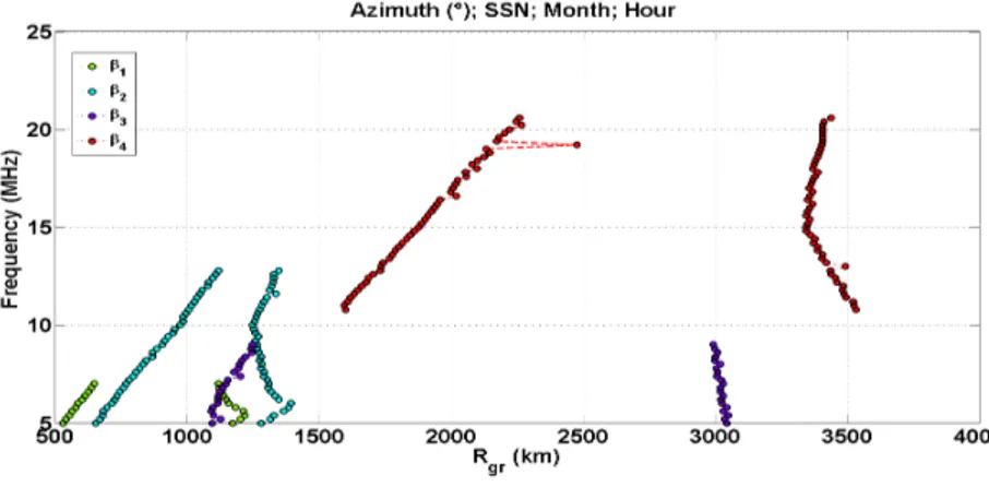
Figure 4.12 shows an example of the surveillance area divided into iso-MTF cells obtained from the iso-MTF curve of the IPC in Figure 4.9; each point corresponds to a lower extreme of cell with a width in ground range equal to ∆R (red box) and for each cell the elevation angle and MTF pair is shown (blue box).
Figure 4.12: Example of iso-MTF cells
It is worth noting that the number of iso-MTF cells is in this case reduced to 3, with a huge save of computational load.
Once the iso-MTF cells have been determined, the scan frequency sets are calculated as follows:
• For a given iso-MTF cell, and referring to the distances that are illuminated by each ele-vation angle βj , the minimum and maximum frequency [ fmj , fMj ] are evaluated. In
Fig-ure 4.13, an example of a given iso-MTF cell is shown. Two frequency sets [ f0m, f0M], [ f1m, f1M] in correspondence of β1and β2are obtained;
• The final outcome of the frequency scanning block will be arranged as a set of el-evation angles - frequency intervals for each iso-MTF cell, {βp(k), [ fpm(k), fpM(k)} ,
k= 0, 1, 2, ..., Nisoand p ∈ [0, 1, 2, ..., N(ϑ ) − 1].
The Figure 4.14 illustrates each step of the above method:
Figure 4.14: Example of frequency - elevation pairs for each iso-MTF cell
1. The extremes of iso-MTF cells in ground range, are determined: Rgr[i];
2. Assuming that f1, f2, ..., fN(ϑ ) are the available frequencies starting from β1(ϑ ), its
foot-print ( Rgr[β1(ϑ , ¯f) + ∆β (β1(ϑ , ¯f))/2] and Rgr[β1(ϑ , ¯f) − ∆β (β1(ϑ , ¯f))/2]) is evaluated
varying ¯f within of those which available (blue and green lines).
The equation 4.10 reports the frequencies - elevation pairs that allow to cover totally the first cell, that extend from Rgr[1] to Rgr[2].
β1(ϑ , ¯f) with f¯= f1, f2, f3, f4 (4.10)
3. Repeating the procedure for the second cell (from Rgr[2] to Rgr[3] ), the pairs that have a
footprint which contains the entire cell are (equation 4.11):
Once the iso-MTF cells in range and the respective set of frequencies have been determined, the optimum frequency can be selected for a fixed radar look direction by using the best radar return as explained in the following paragraph.
4.5.3
The Transmitted Frequency Selection System
The task of this system is to select the transmitted frequency according to the following ap-proach:
1. For a given kth iso-MTF cell, low noise channels are determined within each frequency interval [ fpm(k), fpM(k)];
2. Choose as the transmitted frequency for the k-th iso-MTF cell, the one providing the strongest radar return. As there is no a priori knowledge about the presence of the target, this choise is made by taking into account the normalized Clutter-to-Noise ratio (CNRN
-equation 4.12) rather than of the Signal-to-Noise ratio.
CNRN(ϑ , βm(ϑ ), fj(m, k)) = = 4πgt(ϑ , βm(ϑ ), fj(m, k))gr(ϑ , βm(ϑ ), fj(m, k))σc(ϑ , βm(ϑ ), fj(m, k))( fj(m, k)) 2 c2L2 p( fj(m, k)) N0( fj(m,k)) 2 (4.12) where:
• βmis an elevation angle belonging to set {βm, m = 1, 2, 3, ..., M(ϑ )} relative to kth
iso-MTF cell;
• fj(m, k) is one frequency belonging to set of frequencies that together βm allows to
cover totally the kth cell ;
• σc is the contribution related to percentage of ground and sea, present into
illumi-nated cell (equation 4.13).
σc= σ0,seaAsea+ σ0,groundAground (4.13)
where σ0,sea is the Radar Cross Section (NRCS) per unit area related to the illuminated
Aground are the same quantities but related to the area of illuminated ground surface. The RCS of both land and sea, is dependent on grazing angle and the operating frequency.
Figure 4.15: NRCS for horizontal polarization
Graphics in Figure 4.15 and Figure 4.16 show the plots of NRCS for several types terrain as a function of grazing angle and for both horizontal and vertical polarization respectively [28], while the dependence of NRCS sea is reported in Figure 4.17-[29].
Figure 4.17: Sea NRCS plot
3. For any azimuth angle, the final output will be a transmission parameter table also called Operative Frequency Table - (OFT), organized as the template of Table 4.2.
Data based on CNRN Antenna Footprint
iso-MTF cell number lower extreme cell in km cell extension in range in km upper extreme cell in km frequency in MHz elevation angle in (◦) Rm(f,β ) in km RM(f,β ) in km 1 ... ... ... ... ... ... ... 2 ... ... ... ... ... ... ... ... ... ... ... ... ... ... ...
Table 4.2: Output Table Template for a given azimuth ϑ
For each iso-MTF cell, there are the pairs of elevation angle and the frequency to be transmitted for illuminating the ground points belonging to that cell. Other information regarding the iso-MTF cell, initial and final distance and extension as well as ground range antenna footprint are shown.
Chapter 5
Adaptive Waveform Algorithms
Waveform parameters must be defined in order to meet the system requirements in terms of detection and ground range coverage as well in term of system constraints.
In the following paragraphs a new technique for HF-OTH skywave radar will be defined and analyzed.
The main task of this technique is to set the waveform parameters in a cognitive way as a function of operating conditions, in order to meet the ionospheric conditions, the noise level and the frequency allocation plan.
Figure 5.1 shows the architecture of the waveform parameters setting technique.
In particular the paragraphs that follow will focus mainly on the description of the Waveform Selection block.
Before proceeding with the description of the technique, different encoding classes are compared in terms of immunity to Doppler and robustness to amplitude and phase distortions caused by power amplifier non linearities.
5.1
Transmitted Waveform Model
For any given azimuth direction, the HF-OTH skywave radar must cover distances from about 500 − 600km up to 3000 − 3500km. Typically, several carrier frequencies must be transmitted, and a suitable signal bandwidth is needed to obtain the required radar range resolution. Several waveform models have been proposed in existing systems, namely mono-static planar array Nostradamus system making use of chirp pulses [8]-[9] and the Jindalee Operational Radar Network (JORN), which is composed of two systems of bistatic radars transmitting a LFM-CW signal [4]-[5]; on the basis of what is described in chapter two, a brief summary of existing radar waveforms is shown in Table 5.1.
Wavefom Frequencies Range - (MHz) Band (KHz) PRF (Hz) Max Transmitted Power (kW) JORN LFM/CW 5 − 28 4 − 80 4 − 80 300 Nostradamus Chirp 6 − 28 − − 50 ROTHR LFM/CW 5 − 28 4.7 − 100 5 − 60 200
Table 5.1: Characteristic Parameters of the Waveforms in Radar Systems in use
We refer to a monostatic radar configuration and a multi-frequency pulse-code signal. The possible transmitted signal models for a fixed azimuth angle (ϑ ) and for a given elevation angle (βm(ϑ ), m = 1, 2, ..., M(ϑ )) are following reported.
5.1.1
Pulsed Waveform Instantaneous Multifrequency (IM)
The mathematical expression of the signal is (equation 5.4):
ST(t) = K−1
∑
k=0 Nf−1∑
n=0 xn(t − kTR) exp[ j2π fn(t − kTR)] (5.1) Where:• TR is the pulse repetition time (PRT);
• fnis the carrier frequency;
• Nf is the number of transmitted frequencies;
• K is the number of transmitted pulses;
• xn(t) = A exp[ jφ (t)]rect(Tti) is the complex envelope of the transmitted pulse;
• Tiis the pulse-time length.
Specifically φ (t) is the instantaneous phase of the transmitted signal that depends on what type of encoding used.
In the case of:
Chirp Pulse:
φch(t) =
πnt2
Ti
(5.2) with Bnpulse bandwidth relative to the frequency fn;
Phase Coded: φpc(t) = Kn 2 −1
∑
k=−Kn2 2πa(k) L rect( t− (k + 0.5)Ti kn Ti kn ) (5.3)where a(k) belonging to set I = (0, 1, 2, ..., L − 1) is a multilevel code with L elements and knis
the length of phase code for transmitted pulse.
It is worth noting that the bandwidth of pulse, is variable with "n" because of depends on the available band for the carrier frequency.
When possible, in order to avoid having different resolutions in slant range from one cell iso-MTF to another , the same bandwidth for all frequencies is shall use.
Figure 5.2: Pulse-Code Instantaneous Waveform
The advantages of this signal are that it is possible to optimize the resource time by sending multiple frequencies, with no theoretical limit on the maximum number of them. At the same time, this signal can give rise to spurious and / or harmonic frequencies due to intermodulation phenomenon arising from non-linearity of amplifiers. However, this phenomenon should be contained because of the commercial systems operating in the HF band are used for long distance communication, where the linearity requirements are stringent enough.
5.1.2
Pulsed Waveform SeQuential Multifrequency (SQM)
In this case the analytical expression is:
ST(t) = K−1
∑
k=0 Nf−1∑
n=0 xn(t − nTf− kTR) exp[ j2π fn(t − nTf− kTR)] (5.4)Where Tf is the frequency repetition time, that as it is evident from the Figure 5.3, must be
greater than Tiand such that NfTf ≤ Tskip, where Tskipis the time interval during which it is not
Figure 5.3: Pulse-Code Sequential Waveform
The key advantage of this waveform is the absence of inter-modulation effects, because the frequencies are transmitted separately in time. Remains the constraint on the maximum number of frequencies, which reduces to a few units by limiting the degrees of freedom in transmission.
5.2
Pulse Compression by Encoding
The pulse waveforms are suitable for monostatic radar configurations. However, together with a pulse code, techniques of pulse compression are needed. In fact these allow to obtain a good compromise between range resolution and radar performance..
In fact, a resolution δ R = cTi
2 of 5km would require a pulse duration Ti equal to 33µs, which
would mean transmitting a peak power (A2/2) too high to get a good detection to receiver which is strength correlated with the signal energy (E =A22Ti).
Through the pulse compression, the range resolution is not proportional to Ti, but depends
on the band (B) of received signal. For this reasons, it is possible to separate the needs relative to detection from those relative to range resolution.
The resolution obtained with pulse compression, is the same that of a no-modulated pulse of duration Ti
D where D is the compression ratio (equation 5.5):