ALMA MATER STUDIORUM - UNIVERSITÀ DI BOLOGNA
SCUOLA DI INGEGNERIA E ARCHITETTURA
DIPARTIMENTO DI INGEGNERIA CIVILE, AMBIENTALE E DEI MATERIALI
CORSO DI LAUREA IN INGEGNERIA PER L’AMBIENTE E IL TERRITORIO
TESI DI LAUREA in
Modellistica Idrologica
GROUNDWATER RECHARGE ESTIMATION IN A DATA SPARSE
ARID CATCHMENT OF WESTBANK
STIMA DELLA RICARICA DELLE FALDE ACQUIFERE IN BACINI ARIDI E CARENTI DI OSSERVAZIONI IDROMETRICHE: IL DARGA IN CISGIORDANIA
CANDIDATO RELATORE:
Alessandro Gigliotti Chiar.mo Prof.
Attilio Castellarin CORRELATORE: Chiar.mo Prof. Ralf Merz Anno Accademico 2012/13 Sessione II
2
Index
SOMMARIO ESTESO ...5
1. INTRODUCTION ...10
2. CONCEPTS OF HYDROLOGICAL MODELING ...12
2.1 Hydrological Variables and Models...12
2.1.1 Basic concepts ...12
2.1.2 Classification of hydrological models ...14
2.1.3 Calibration and validation ...15
2.2 Predictions in ungauged basins ...16
3. DESCRIPTION OF THE STUDY AREA ...19
3.1 Climate: ...20
3.2 Geology ...22
3.3 Soils ...23
3.3.1 Soils in North of Darga catchment...25
3.3.2 Soils in South of Darga catchment...27
3.4 Land cover ...28
4. DESCRIPTION OF THE MODEL ...30
4.1 Model’s structure ...30
4.2 Model output...34
4.2.1 Evapotranspiration ...34
4.2.2 Soil water budget ...38
4.2.3 Snow cover ...38
4.3 Model’s parameters ...39
3
5.1 Meteorological input data ... 41
5.2 Catchment’s input data ... 44
6. GIS-BASED HYDROLOGICAL ANALYSIS ... 47
6.1 Management of information in a GIS system ... 47
6.2 Basic definitions ... 47
6.3 Derivation of Darga catchment’s shape ... 49
7. CALIBRATION ... 59
7.1 Evapotranspiration ... 63
7.2 Groundwater recharge... 66
7.3 Runoff ... 72
8. VALIDATION AND EFFICIENCY ... 73
8.1 Groundwater recharge estimation using Chloride mass-balance ... 73
8.2 Runoff ... 77
9. RESULTS ... 79
10. CONCLUSIONS ... 84
APPENDIX: Matlab’s scripts ... 86
A.1 Aridity index Calculation ... 86
A.2 Chloride Mass-Balance implementation... 87
A.3 Daily Actual Evapotranspiration ... 90
A.4 Actual and Potential Evapotranspiration ... 91
A.5 Groundwater Recharge ... 95
A.6 Monthly Actual Evapotranspiration from different sources and Soil Moisture ... 99
A.7 Runoff comparison ... 102
A.8 Soil Moisture ... 105
4
5
SOMMARIO ESTESO
Il seguente elaborato è frutto del lavoro di ricerca, della durata di cinque mesi, svolto presso il Department of Catchment Hydrology del centro di ricerca UFZ (Helmholtz-Zentrum für Umweltforschung) con sede in Halle an der Saale, Germania. L’obiettivo della Tesi è la stima della ricarica della falda acquifera in un bacino idrografico sprovvisto di serie di osservazioni idrometriche di lunghezza significativa e caratterizzato da clima arido. Il lavoro di Tesi è stato svolto utilizzando un modello afflussi-deflussi concettualmente basato e spazialmente distribuito. La modellistica idrologica in regioni aride è un tema a cui la comunità scientifica sta dedicando numerosi sforzi di ricerca, presentando infatti ancora numerosi problemi aperti dal punto di vista tecnico-scientifico, ed è di primaria importanza per il sostentamento delle popolazioni che vi abitano. Le condizioni climatiche in queste regioni fanno sì che la falda acquifera superficiale sia la principale fonte di
approvvigionamento; una stima affidabile della sua ricarica, nel tempo e nello spazio, permette un corretta gestione delle risorse idriche, senza la quale il fabbisogno idrico di queste popolazioni non potrebbe essere soddisfatto.
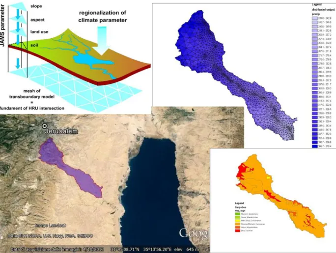
L’area oggetto di studio è il bacino idrografico Darga, una striscia di terra di circa 74 km2
, situata in Cisgiordania, la cui sezione di chiusura si trova a circa 4 kilometri dalla costa del Mar Morto, mentre lo spartiacque a monte, ubicato a Nord-ovest, dista circa 3 kilometri dalla città di Gerusalemme (figura 1).
6
Figure 1.(partendo in basso a sinistra e muovendoci in senso orario) Ubicazione del bacino idrografico Darga. Illustrazione del metodo della discretizzazione dello spazio in HRU (unità di risposta idrologica). Assegnazione di valori medi annuali di precipitazione per ogni HRU. Caratterizzazione geologica del bacino.
La prima parte del lavoro si è incentrata sullo studio del bacino idrografico dal punto di vista climatico e geomorfologico, al fine di individuare e collezionare tutti i dati geomorfologici e climatici necessari alla modellazione numerica. La zona in esame è caratterizzata da
condizioni di clima arido, con alte temperature medie annuali (25°C) e valori di evapotraspirazione potenziale giornaliera (7.39 mm) di molto superiori a quelli di
precipitazione (0,86 mm). La distribuzione degli eventi di pioggia si organizza in brevi ed intensi temporali alternati a lunghi periodi di tempo secco; inoltre, va sottolineato come il bacino in esame sia assai carente in termini di misure idrometriche. Tali problematiche hanno reso la modellazione idrologica di quest’area una sfida particolarmente impegnativa poiché si
7
sommano le difficoltà legate alla studio idrologico di un area carente di acqua a quelle legate all’utilizzo di un modello in un area carente di misure. La classica procedura di calibrazione-validazione di un modello matematico di trasformazione afflussi-deflussi, effettuata
confrontando la curva delle portate osservate con quella simulata dal modello, non è percorribile nel caso in esame, disponendo per il bacino di sole misure di portata sporadica (42 giorni su di un arco temporale di 10 anni).
Lo studio ha permesso di implementare una strategia di calibrazione alternativa, chiamata “multi-response calibration”. Tale strategia è basata sull’utilizzo di differenti variabili misurate localmente ed in remoto (da satellite) con l’obiettivo di ottenere con un unico set di parametri del modello matematico una riproduzione accurata di un insieme di osservazioni di variabili idrologiche di diversa natura simulate dal modello. In particolare, la procedura si è concentrata sulla corretta riproduzione da parte del modello dell’evapotraspirazione
potenziale ed effettiva, dell’umidità del suolo e della ricarica della falda acquifera. Su quest’ultima variabile è stata posta un’attenzione particolare, essendo la sua stima affidabile il fine ultimo di questo lavoro di modellazione idrologica. Al fine di ridurre il più possibile errori ed incertezze necessariamente legati ad una procedura di calibrazione-validazione non convenzionale, sono stati utilizzati due differenti metodi di calcolo della ricarica della falda acquifera, uno in calibrazione e uno in validazione. Durante la fase di calibrazione è stata utilizzata l’equazione di“Guttman and Zukerman”, calibrata per le aree aride e già utilizzata con successo in Medio Oriente (Guttman & Zukerman, 1995). Detta procedura lega la ricarica della falda acquifera al valore della precipitazione tenendo conto dell’intensità
dell’evento. Per la fase di validazione si è invece utilizzato un metodo ancora più preciso, che è il bilancio di massa del cloruro; la ricarica della falda acquifera è stata stimata in funzione della pioggia e della concentrazione di cloruro contenuta nelle acque piovane e in quelle sotterranee. La precisione del metodo e il suo basarsi su dati raccolti in campo ne
determinano un’affidabilità comparabile a quella di osservazioni dirette dei movimenti della falda acquifera. La bontà del modello nel simulare andamenti delle variabili di interesse comparabili a quelli reali è stata misurata utilizzando diverse funzioni obiettivo (ad es. efficienza di Nash -o coefficiente di determinazione-, R2, Errore Medio Relativo).
8
La struttura della Tesi ricalca fedelmente le fasi in cui il lavoro di ricerca è stato suddiviso, articolandosi in 10 capitoli:
- Il primo capitolo è un introduzione al problema del sostentamento del fabbisogno idrico in Cisgiordania; vengono descritti gli scopi del progetto, gli strumenti che sono stati utilizzati e le problematiche incontrate.
- Il secondo capitolo espone i concetti teorici di base e le definizioni fondamentali della modellistica idrologica, elementi funzionali alla comprensione dell’elaborato.
- Il terzo capitolo è un analisi approfondita e dettagliata del bacino idrografico in esame. L’area viene descritta dal punto di vista climatico, geologico e pedologico con particolare attenzione alle caratteristiche che influenzano il processo idrologico. - Il quarto capitolo contiene la descrizione del modello idrologico spazialmente
distribuito a base concettuale utilizzato nello studio, J2000g ottenuto come
semplificazione del modello più complesso J2000 (Krause, 2009), ne viene descritta la struttura, il significato dei parametri che governano il calcolo delle variabili e gli output che genera.
- Il quinto capitolo descrive il processo di raccolta e sistematizzazione degli input necessari a far girare il modello, esso descrive le fonti da cui i dati provengono e la loro natura, da quelli di tipo climatico a quelli legati a topografia, pedologia, idro-geologia e uso del suolo.
- Il sesto capitolo fornisce la descrizione del lavoro svolto in ambiente GIS per
effettuare l’analisi idrologica dell’area in esame ed estrarre lo spartiacque del bacino idrografico partendo dalla conoscenza della posizione della sezione di chiusura del bacino stesso e da un modello digitale delle quote del terreno della regione in esame. - Il settimo capitolo riguarda la fase di calibrazione del modello, viene illustrata la
strategia alternativa di calibrazione utilizzata nello studio.
- L’ottavo capitolo descrive la fase di validazione del modello e la valutazione dell’efficienza, in particolar modo si concentra sulle variabili di confronto utilizzate nella strategia di validazione e sulle funzioni obiettivo considerate per valutare l’affidabilità predittiva del modello.
- Il nono capitolo riporta una descrizione dei risultati ottenuti, vengono mostrati e commentati gli output spazialmente distribuiti delle variabili di interesse.
9
- Il decimo capitolo si concentra sulle conclusioni del lavoro, vengono discussi i risultati ottenuti e proposti miglioramenti tecnici.
- L’ultima parte dell’elaborato è un appendice contenente la lista degli script creati in Matlab per portare a termine le fasi di calibrazione, validazione e valutazione della bontà del modello.
10
1. INTRODUCTION
A wise water resource management is of high importance in areas characterized by water shortage, where water is an extremely valuable resource, and cannot be wasted. According to the Palestinian water Authority the quantity of water used for domestic purpose in West Bank in 2003 was 64.7 × 10⁶ m3, which averaged over a population of 2,313,609 (Marei et al., 2010) means roughly 86 l per person without considering the water losses associated with water transportation, which suggests that the true value is probably significantly lower. If one compares this value with the amount of water recommended by the World Health
Organization, 150 l per person, he/she can easily understand why water resource
management is so important in this area of the world. Moreover, in addition to the water shortage, a large number of Palestinian communities are not connected to the water supply systems networks. Groundwater is actually the most important source of fresh water in the area.
The main aim of this Dissertation is trying to make a reliable estimation of groundwater recharge in an arid catchment of Israel, which is ungauged in the sense that no direct runoff measurements are available for the study catchment. Some of the most used and well established techniques to extract useful information from areas with lack of data are
presented herein, and the dissertation also present a general discussion on some of the most problematic situations hydrologists have to face in cases like this.
The present study considers a conceptual spatially distributed hydrological model, working at a daily temporal resolution. Input data comes from local authorities, previous field
inspections and, where missing, literature values. The study shows that the model J2000g, under an appropriate parameterization, is able to describe at daily time step the replenishment of the aquifer along with other hydrological variables such as actual evapotranspiration, soil moisture, etc.. The goodness of the model’s performance is assessed by comparing the distributed variables with the corresponding measured or theoretical (i.e. expected) values, where possible, and by performing an analysis of precision and efficiency. All the
11
managed and analyzed within a GIS (Geographical Information System) environment (ArcGIS® software), while Matlab® scripts were specifically written for plotting results and calculating efficiency factors. The scripts are attached and commented in an Appendix. Estimation of groundwater recharge in this area is a challenging goal because we had to face the sum of three different problems:
- Implementation of hydrological modeling in arid and semi-arid areas, where
precipitation is absent in most part of the year and it occurs only in few short and very intense events with the form of thunderstorm.
- Predictions in ungauged basins: the almost total absence of runoff data leads to the impossibility to apply a normal calibration-validation strategy, based on comparing simulated runoff with observed series. Another strategy for calibrating and validating the model, based on a multi-response comparison of different hydrological variables, was identified and used.
- Information comes from different sources and several data are affected by large uncertainty and measurement errors (e.g. daily temperature values from Israeli meteorological service, IMS).
This study borders some of the most difficult, and still open, problems of hydrology and, thanks to some necessary assumptions and simplifications, demonstrates the possibility to make reliable predictions and extract useful information from and for this area.
12
2. CONCEPTS OF HYDROLOGICAL MODELING
2.1 Hydrological Variables and Models
2.1.1 Basic concepts
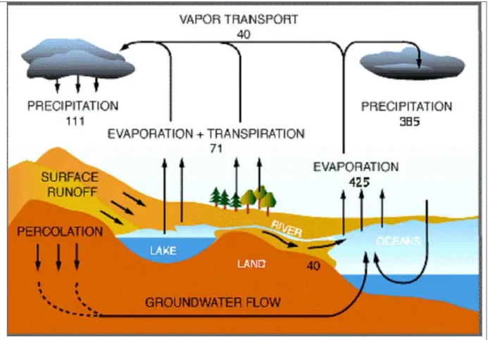
Hydrology is the study of hydrologic cycle, water resources and environmental watershed sustainability on the Earth. Qualitatively the hydrological cycle at Earth scale is composed by the following main phenomena (figure 2.1):
- Precipitation: can be liquid or solid, it has high variability in time and space. - Interception: amount of water that does not reach the soil, but is instead intercepted
by the leaves and branches of plants and directly evaporates from them. - Evaporation: water vapor that returns from the surface again to the atmosphere - Transpiration: water vapor that returns the atmosphere due to plants life-cycle - Infiltration: amount of water that reaches the soil and penetrate it due to gravity and
capillarity forces. It doesn’t become surface flow.
- Percolation: is the infiltration in the deeper layers, in permeable rocks, until reach groundwater storage.
13
Figure 2.1 Hydrological cycle, Values in 103 km3/yr (http://www.globalchange.umich.edu).
A hydrological model is a system of mathematical equations with the aim of simulates part of the hydrologic cycle. It is used to calculate one, or more, hydrological variables. A
hydrological variable is a real (or integer) number characterizing a physically observable quantity in a hydrological process. Although it is a deterministic quantity it is usually described stochastically because lot of hydrological phenomenon are not perfectly known or we do not have the instruments to described them mathematically.
A model is characterized by input variable, output variable, state variable and parameters: - Input variable: what we introduce in the model, known data about the phenomenon
from which depends the quantity we want to estimate,
- Output variable: what we want the model to calculate; it is the quantity we want to estimate,
14
- Parameters: describe proprieties of the system, can be constant or vary in function of time.
Equations of the model basically describe exchanges of water volumes under two principles from fluid mechanics:
- Conservation of mass; - Conservation of energy.
2.1.2 Classification of hydrological models
Application of Hydrological models has three main purposes: Calibration, Prediction and Solution of Inverse Problems.
- Calibration: we have knowledge of input and output variables and we want to find the best parameter set.
- Prediction: that is the most common purpose for which models have been developed, we know input and parameters and we want to estimate the output variables.
- Solution of Inverse problems: quite rare in hydrology, it refers to the cases in which there is knowledge of parameters and output and the aim is to calculate the input. Models can be deterministic or stochastic: they are defined as deterministic when at one input correspond always the same output, there are not stochastic processes in the calculations of the output variables. Otherwise they are stochastic if at least one of the variables of the models is governed by a stochastic process, which means the result can change also when the input are the same. As said before this “trick” is used in hydrology to pay the not perfectly knowledge we have about some of hydrologic phenomenon.
Models can also be classified according to their structure, work scale and characteristic of simulation. Regarding structure models can be:
- Physically based: the equations try to describe mathematically the real dynamic of the natural phenomenon. As hydrological phenomena have always spatially variability, physically based models have to be spatially distributed.
15
- Conceptually based: take in account the real dynamic of the phenomenon but make some assumptions and simplifications.
- Black box: equations have nothing to do with the real dynamic of the phenomenon; the only aim is to give realistic output.
Concerning spatial scale models can be:
- Lumped: models work considering the entire basin as a unique spatial unit; variables depend on the time but not on the space.
- Distributed: models divide the basin in spatial units which can be considered homogeneous for hydrologic characteristics; variables depend on both time and space.
- Semi-distributed: models work in sub-basin scale, so each calculation is made for every sub-basin and then the results are propagated to the outlet.
A basin is a topographic area, identified by a close polygon termed watershed, where all the rain falling in the area flows in only one point, which is the outlet of the catchment.
Regarding characteristic of simulation models can operate continuously in time, or be event-based (i.e. reproducing single event). Models which are good in modeling events (e.g. extreme events) are usually not good in the continuous simulation, and models accurate in the continuous prediction usually are not able to well simulate extreme events.
2.1.3 Calibration and validation
In most of the cases it is not possible to directly measure the parameters of the model or to identify reliable parameter values in the literature, usually parameters values have to be adjusted to better fit with observed values. As already mentioned, the process to find the best parameter set is called calibration (figure 2.2). Calibration need the knowledge of input and output data, in the same time step and for the same time period. Model parameters are changed (manually or by using automatic algorithms that minimize or maximize mathematical objective functions) in order to make the output of the model as close as possible to the observations. With the assumption that what happens in the past can guide us in the prediction of what will happen in the future, we suppose that the parameter set found to
16
be the best for the observation period will also be good for the near future, if general conditions in the catchment do not change significantly.
Figure 2.2 Calibration strategy. (Montanari & Castellarin, 2013)
Once identified a suitable parameter set through calibration we have to validate the model, which means check the goodness of its prediction. For this purpose we need another set of data complete of input and measured output, which should be different from the one used during the calibration. Validation ends with comparing the model output with the real one; if the simulated series fit with the measured ones the model is able to make reliable prediction in the catchment.
2.2 Predictions in ungauged basins
Simulation is always subject to uncertainty, mostly because a model does not reflect perfectly the reality and the data available can contain errors. When measured data for calibration-validation are missing, or are sparse and insufficient, uncertainty increases because the
17
goodness of model output cannot be checked properly. Under these circumstances a different strategy for calibration-validation has to be found. This is the case of prediction in ungauged basins (PUB).
An ungauged basin is a catchment with inadequate records (Sivapalan et al., 2010), the inadequacy can be in terms of quantity or quality of the data and it makes impossible to calculate the variables of interest in the appropriate spatial and temporal scale and with acceptable accuracy for practical applications. For example if the variable of interest has not been measured for the required time period, or with the wrong resolution the basin would be classified as ungauged with respect to this variable.
In fact, in order to make certain predictions, Hydrological modeling always requires the proper identification of three main components:
- A model that can describe hydrological processes,
- A set of parameters that describe the basin’s proprieties that mainly drive the processes we want to study,
- An appropriate meteorological input.
These components can be not all perfectly known or, in the worst case, not known at all because of the space and time heterogeneity. A prediction in ungauged basin is the
prediction, and its associated uncertainty, without using the past time series of the variable that is being predicted, so without the possibility to make a direct calibration. Also
validation, comparing results with observed data, is not possible and that means predictions in these cases cannot be verified with confidence, so they are always affected by uncertainty. The uncertainty in the prediction does not come only from lack of validation, but also from the process of prediction due to lacks in its components. That is because there is
heterogeneity in the climate variable, in the landscape and in the dynamic of processes, which cannot be perfectly described by the prediction system. There are three kinds of uncertainty:
- Uncertainty in model structure (i.e. the model cannot correctly reproduce the landscape space)
18 - Uncertainty in climatic input
The prediction in ungauged basin is generally most focused on water quantity and availability problems (flood flows associated with a given exceedance probability, soil moisture, groundwater recharge, low-flow variability, etc.) because water quality problems need the knowledge of the flow partitioning to be solved. We also focus on quantitative aspects of the water cycle in the basin, as our goal is to predict the groundwater recharge continuously in time and distributedly in space.
19
3. DESCRIPTION OF THE STUDY AREA
The West Bank is a territory located in Western Asia. It is geographically included in the state of Israel, meaning that West Bank shares boundaries with the state of Israel to the West, North, and South, while to the East, across the Jordan River, it shares boundaries with Jordan and part of the west Dead Sea coastline. Regarding similitude in climate,
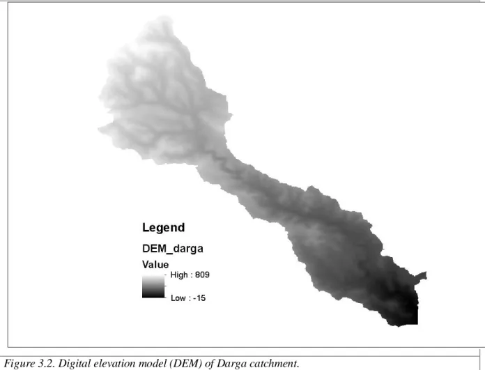
hydrogeological characteristics and land cover West Bank can be divided in three parts: Western, Eastern and Northeastern. Focusing on groundwater movement in the mountain area, three groundwater basins were identified; one in each zone (Marei et al., 2010). The Dead Sea has an elevation of 410 m below the sea level and is the lowest part of West Bank. The Darga catchment, which is the study basins, is a strip of land of 73.926.900 m2, situated in the Eastern part. Its outlet is situated at about 4 km from the Dead Sea shoreline and the higher part of the catchment is situated 3 km far from the city of Jerusalem (figure 3.1). Its elevation ranges between 809 meters above the sea level in the north-west of the catchment and 15 m below the sea level in the south-east part, in correspondence of the outlet (figure 3.2).
20
Figure 3.2. Digital elevation model (DEM) of Darga catchment.
3.1 Climate:
The climate in West Bank is mostly controlled by three factors: the distance from the sea, the distance from the deserts and the elevation from sea level. The Mediterranean Sea influences the humidity, the fluctuation of temperature and the amount of rainfall. Near the deserts humidity decreases, mean temperature (daily and seasonal) increases and precipitation decreases. Elevation affects the climate by increase rainfall and decrease humidity; mean temperature also decrease with elevation.
The climate change from semi-humid in the western side to the arid in the eastern, in fact precipitation is above 600 mm/year on the mountain ridge and below 100 mm/year on the Dead Sea Shore (Palestinian Water Authority). The rain events occur mostly during the
21
winter and spring seasons, and during events of high intensity, i.e. more than 50 mm per day or more than 70 mm in two days (Raffety, 1965), surface runoff is observed.
August is the warmest month of the year and the mean temperature can reach 34°C along the Dead Sea shore. January is the coldest month and the mean temperature is around 16°C near the Dead Sea but far from it, in the western part, can also go below 10°C.
Darga catchment is situated in the eastern zone and reflects this trend. Precipitation is higher in the west part (that is also the upper part), almost linearly decreases in the east part and has a minimum near the Dead Sea shore. Annual precipitation ranges between 200 and almost 400 millimeters, it has a high variability in space and time.
Climate condition of the catchment can be described as arid. In reality it is difficult to derive a unique and practical definition of arid environments because they are extremely diverse in terms of land forms, soils, fauna, flora, water balance and human activities (The Food and Agriculture Organization of the United Nations, 1989). Usually aridity is expressed as
function of precipitation and potential evapotranspiration, one of the most used indexes is the climatic aridity index: P/PET, where P is precipitation and PET is potential
evapotranspiration calculated by the method of Penman. Depending of the value of these index arid areas can be divided in three categories:
- Hyper arid zone: arid index 0.03 or lower. Usually they are dryland areas without vegetation, with the exception of few shrubs. Annual rainfall is low, usually not higher than 100 millimeters, and it occurs in irregular and infrequent way. Often there are period, also longer than year, without rain and after short period of intense
precipitation with the form of thunderstorm.
- Arid zone: arid index ranges between 0.03 and 0.20. It is characterized by sparse native vegetation, usually shrubs, herbaceous and small threes; the presence of farm is possible only if artificial irrigation is available. Precipitation is characterized by high variability, with annual sum ranging between 100 and 300 millimeters.
- Semi-arid zone: arid index between 0.20 and 0.50. Native vegetation is quite various, with lot of species. Annual precipitation varies a lot depending on the season: in winter it range between 200 to 500 millimeters and in summer between 300 and 800.
22
Rain is enough to support agriculture with not too high level of production without the help of artificial irrigation.
- Sub-humid zone: arid index between 0.50-0.75. It is not a properly humid zone so it is also classified in the term “arid zone” because in it is possible to find condition
typical of arid climate.
Darga catchment has an average daily PET of 7.39 mm and an average daily rain of 0.86 mm, the value of aridity index is 0.12 which means it is an arid area. Values of annual precipitation also confirm that, because they range between 200 and less than 400 mm and the precipitation occurs mostly in winter moths with short intense thunderstorms spaced by long periods of completely dry conditions.
3.2 Geology
Eastern part of Israel is characterized by erosive activity, increased by the difference between the elevation of Dead Sea and the Mediterranean Sea (Arieh Singer, 2007). There are five aquifers within the Eastern basin. The main one is the Judea Group aquifer, which consists of limestone and dolostone of Early Cenomanian to Turonian age. The secondary aquifers consist of limestone and chalk of Eocene age in the Samaria syncline, basalt of Neogene-Quaternary age in the lower Galilee area, alluvium fill of Neogene-Neogene-Quaternary age in the Bet She'an area and the Jordan Valley, and limestone of Jurassic age. (Geological survey of Israel)
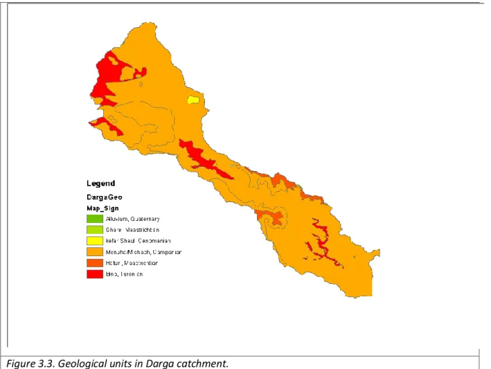
Darga Geology is characterized by sparse formations of Limestone, marl and dolostone from the Turonian age (“Bina” in figure 3.3) but most part of the geological formation is
composed of a mixture of Menuha and Mishash from Upper Cretaceous age (figure 3.3). Mishash is mostly composed of chalk, phosphorite, massive chert and fossiliferous limestones. Menuha is composed of dolomite, bitumen, phosphor, silty chalk and chert. Percent of the composition can vary in function of the geographical location.
Every geological unit has hydraulic proprieties which influence qualitatively and quantitatively the dynamic of groundwater recharge in the catchment. Mishash is rather permeable, so it has the proprieties of an aquifer, where aquifer is defined as a layer of permeable rock or unconsolidated materials from which groundwater can be extracted.
23
Menuha has low permeability so it is defined as having the proprieties of an aquitard. Bina is the name of a geological formation really common in Israel characterized by high
permeability; it can be divided in Deronim, Shivta and Nezer formations (Dan, 2001).
Figure 3.3. Geological units in Darga catchment.
3.3 Soils
Soil distribution in Israel generally follows lithology and topography. Here is presented a short description of the soils of Darga catchment; however the area is not really big there is a difference between north and south. Soils influence also hydraulic characteristics of the catchment, that is why it is important to know which soil type can be observed in each part of the basin. The difference in presence of soils also reflects the difference of climate
conditions, in fact in the Northern portion of the catchment can be found soils which usually occur in semi-humid or humid conditions, otherwise in the south there is presence of soils
24
typical of arid conditions. All the soil types will be described focusing on composition, conditions in which occur, classification in two different systems, USDA and FAO, color (in order to be able to recognize them in field) and hydraulic proprieties. Particular attention is given to the content of clay, sand and silt of every soil type which highly influences
hydraulic characteristics such as porosity and hydraulic conductivity. So it’s useful to remember that:
- Clay: d < 0,002 cm,
- Silt: 0,002 cm < d < 0,05 cm, - Fine Sand: 0,05 cm < d < 0,25 cm, - Coarse Sand: 0,25 cm < d < 2 cm, Where d is the grain size (diameter).
The USDA Soil Classification is an elaborate classification of soil types developed by United States Department of Agriculture and the National Cooperative Soil Survey that groups soils in several levels according to their properties.
FAO soil classification is a supra-national classification, also called World Soil
Classification, developed by The Food and Agriculture Organization of the United Nations (FAO) which offers useful generalizations about soils pedogenesis in relation to the
interactions with the main soil-forming factors. Many of the names used in this classification are known in many countries and do have similar meanings worldwide.
An average value of bulk density is estimated for this area by the World Soil Classification, and it is 1.49 kg/dm3; bulk density is a really important parameter to take in account in some compaction process, usually involving vibration of the container, and it is defined as the mass of many particles of the material divided by the total volume they occupy. The total volume includes particle volume, inter-particle void volume, and internal pore volume. Bulk density is not an intrinsic property of a material; it can change depending on how the material is handled.
25
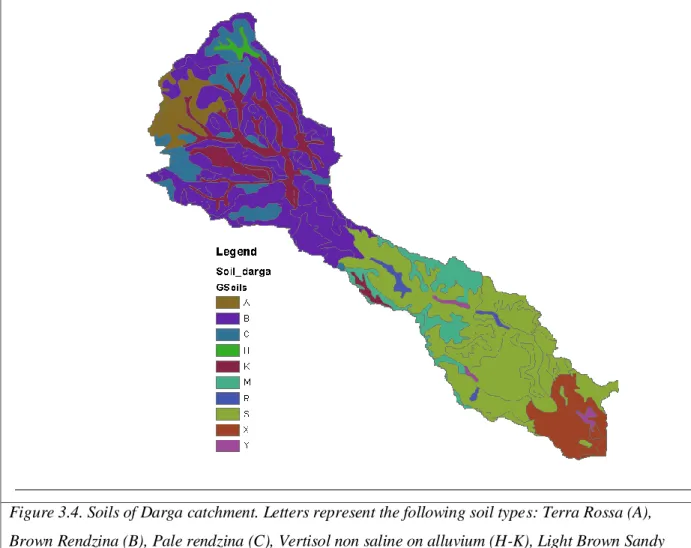
Figure 3.4. Soils of Darga catchment. Letters represent the following soil types: Terra Rossa (A), Brown Rendzina (B), Pale rendzina (C), Vertisol non saline on alluvium (H-K), Light Brown Sandy Loam (M), Loess Serozem (R-S), Reg Soil (X-Y).
3.3.1 Soils in North of Darga catchment
As said before, distribution of soils, as it occurs for geology, change a lot between north and south. North of Darga catchment is characterized by Terra Rossa, Brown Rendzina and Pale Rendzina (letters A, B and C of figure3.4). The first one is present in limestone and dolomite; Rendzina soils are found mostly on chalk and marl. There is also a sparse presence of
Vertisol non saline, on alluvium. (H and K in figure 3.4)
In the USDA soil classification, Terra Rossa would be classified as Rhodoxeralf or Haploxeroll, in the FAO classification as Luvisol. Rendzina in the USDA classification would be classified as Haploxeroll or Xerorthent and in the FAO classification as Rendzina (Arieh Singer, 2007).
26 TERRA ROSSA
Terra rossa is usually found in continuous extended layer, however it is more common in humid climate it can be observed also in arid areas, but with some of its proprieties changed. It is composed by dolomite and limestone from the Turonian age with some calcareous sediment. Its formation is due to the exposition of these rocks to Mediterranean conditions. Soil depth in this area can reach 60 cm and the color varies from brown of the upper horizons to red and dark red in the deeper layers. The content of clay is usually really higher than the content of sand and it increase with the depth; It is always more than 60%, sand is around 10% and the rest is silt. Field capacity is moderate.
PALE RENDZINA
Rendzina soils are rarely continuous and usually mixed with other soil type; in the north of Darga basin they are mixed with Vertisol, which is a colluvial soil, but it is not uncommon to observe Rendzina soils in association with Terra Rossa. Usually Rendzina soils occur on pour calcareous sediments, mainly chalk and marl. As same for Terra Rossa this kind of soils are mostly present in humid climate conditions but a particular soil of the group,
Xerorendzina, is found also in arid and semi-arid conditions. The composition can vary but usually it includes high content of CaCO3 and clay minerals. Depth is moderate: for Pale
Rendzina (Xerorthent in the USDA soil classification) it cannot reach more than 80 cm. the clay content is lower respect to Terra Rossa, around 55%, sand content is around 20%. There are some difference between Pale Rendzina soils developed on chalk and the one developed on marl. The first group usually has lower content of clay, more carbonates and paler color, from light grey in the upper layer to white in the deepest horizon. The second group has color varying from dark grey (higher content of clay) to light yellowish brown. Hydraulic
conductivity of Pale Rendzina soils is good, but it decreases when the clay content increases. BROWN RENDZINA
Brown Rendzina (Haploxeroll in the USDA soil classification) represents an advanced stage of Rendzina soils development (Dan et al., 1972) which occurs when erosion is prevented. It comes from calcareous rocks of moderate hardness and porosity, according to Dan (1976) the formation took place in semi-arid and arid climate conditions due to the precipitation of
27
carbonates, it is usually associated with Nari lime crust. Depth is limited, usually below 30 cm. The color varies from very dark brown to brown in the deeper layers. Clay content is about 45% and sand content between 15 and 25%, it increase with the depth. Porosity is around 35% and conductivity is good as the one of Pale Rendzina, water holding capacity is moderate.
VERTISOLS
In Israel colluvial soils covering wadi beds are not uncommon. These soils can develop on two different rock formations: fine-grained alluvium and basalt, but the formation from alluvium is more frequent (Arieh Singer, 2007). They can be found in a very large range of climate conditions, from humid to arid climate. In the Darga area can be observed few formations of Non-saline Vertisol, developed from alluvium, typical for the area
characterized by arid or semi-arid conditions. For this soil the content of clay reach values of 60%, otherwise the content of sand is quite low, usually around 5%. Depth can be really high, until 150 cm and the color changes from the red-brown in the 0-12 cm horizon until the dark red-brown in the 90-150 cm horizon. Water-holding capacities are high while
infiltration is low, hydraulic conductivity is also low.
3.3.2 Soils in South of Darga catchment
South part of Darga catchment is dominated by the presence of Loess Serozem and Light Brown Sandy Loam (R, S and M in figure 3.4). Near the Dead Sea shoreline, in proximity of the basin’s outlet, there is a heavy presence of Reg Soil. (X and Y in figure 3.4)
LOESSIAL SEROZEM
This soil, typical of arid areas, is composed by Aeolian sediments, according to the most accredited theory originated from desert (Reifenberg, 1947). The color varies from pale brown to yellowish brown depending on the depth, which can be very high, In fact in this area this kind of soil can reach the depth of 190 cm. the content of clay is around 20%, the content of sand 25% in average but it decrease with the depth; in the first layer the content of sand can reaches 35%. Infiltration capacity is moderate but soil moisture movement both in horizontal and vertical direction is rapid.
28 LIGHT BROWN SANDY LOAM
Light Brown Sandy Loam is a closed parent of Loess Serozem; it also comes from Aeolian sediments, after various sedimentation cycles. Is composed mainly by sandy sediments but include however also finer-grained materials of Loessial character. It’s a soil observed mostly in arid areas; the color is very pale brown and doesn’t show big variations. The depth is around 170 cm, which a content of clay that can varies from 90% in the upper layer to 70-80% in the most depth horizon. Content of clay is quite low, about 10% in average. As said for Loess Serozem, the infiltration capacity is moderate but soil moisture movement is rather rapid.
REG SOIL
Reg soils are typical of desert climate conditions, so extremely arid with rare precipitation, usually in the form of thunderstorm. These Soils are composed by limestone, dolomite, chalk, flint and marl, together with some fines materials, the content of CaCO3 is usually
high. The content of clay is about 20% in average but it varies a lot with the depth in a non-linear trend, the content of sand is quite high, about 40% with values that can reach 60% in the deeper horizon. The presence of well-defined soil horizons distinguished Reg soils from other desert soils; in fact it is one of the most stratified soils we can observe in this area. Its depth can reaches 170 cm. the color varies from very pale brown to reddish-yellow.
Infiltration capacity is moderate.
3.4 Land cover
Vegetation is highly influenced by climate; its characterization is important because it affects the process of evapotranspiration and so the hydric balance. Vegetation cover in arid zone is scarce but some plant forms often occur in it and can be classified as:
- Ephemeral annuals, which appear after rain; their growth lasts only in a short wet period and their life usually doesn’t exceed the 8 weeks. They have small size and shallow roots.
- Succulent perennials are able to accumulate and store water and participate to the process of evapotranspiration. Cacti are typical example of succulent perennials.
29
- Non-succulent perennials comprise the majority of plants in the arid zone. These are hardly plants including grasses, woody herbs, shrubs and trees that can hold out the unfriendly conditions of arid areas environment.
Darga catchment’s land cover changes a lot between north and south, reflecting the changing of climate conditions. The lowest part, near to Dead Sea, is almost totally composed of rocks, without vegetation (figure 3.5). In the middle of the catchment can be observed an equal presence of rocks and open soil, so still the vegetation is absent or so rare that could not affect the hydric cycle. Vegetation occurs in the upper part of the catchment (figure 3.5), the one that present higher elevation and higher value of precipitation. In this part a wider variety can be observed: open soil is still highly present but together with sparse vegetation,
agricultural crop, shrubs and plants characterized as deciduous forest. Also a few anthropological presences are distinguished in the map.
30
4. DESCRIPTION OF THE MODEL
4.1 Model’s structure
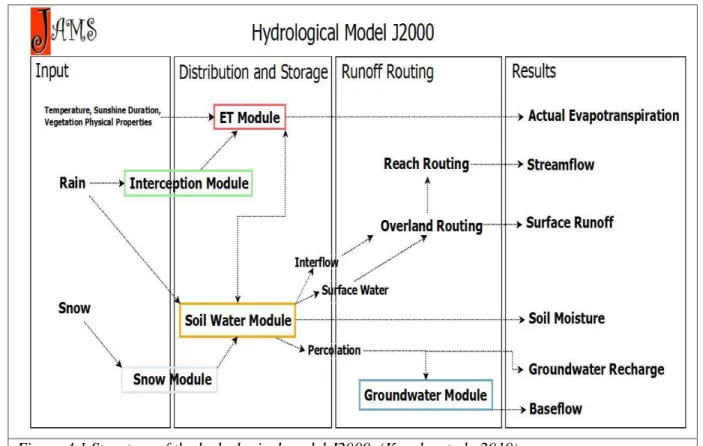
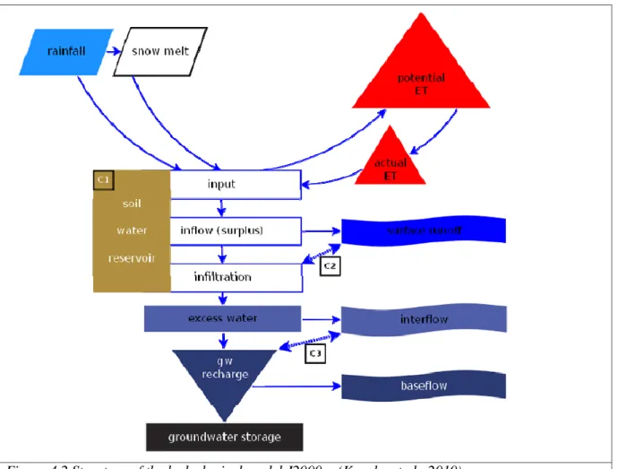
J2000g is a conceptual, spatially distributed, hydrological model. The model is a simplified version of the more complete J2000 model (figure 4.1). It simplifies many of the complex hydrological relationships within J2000 and has a reduced number of parameters to be calibrate. It can calculate temporally aggregated, spatially allocated hydrological target sizes, and works with different discretization strategies, such as response unit, grid cells, and catchment areas. J2000g (figure 4.2) uses a modelling environment called JAMS, Jena Adaptable Modeling System, which is a JAVA-based modeling framework system for the development and application of environmental models. JAMS can be run independently from the operating system in a Java Runtime Environment. (Knoche et al., 2010); it was developed to accomplish three main characteristic (Krause and Kralisch, 2005):
- All process implementation need to be technically independent from the spatial representation of the simulated catchment,
- Spatial and temporal domains can be arbitrary configured by the users,
- The system must be able to integrate process from simple empirical to complex physically based algorithms.
31
Figure 4.1 Structure of the hydrological model J2000. (Knoche et al., 2010)
The model needs spatially distributed information regarding topography, soil, hydro-geology and land use; each information has to be available for every model unit in the catchment, where model units are the areas in which the catchment is divided with the assumption that characteristics in each area can be considered having homogeneity. Then the model needs meteorological input data which have to be in the same time frame in which we want the output to be; the information required is about temperature, humidity, precipitation, wind speed, hours of sun and runoff.
32
Figure 4.2 Structure of the hydrological model J2000g. (Knoche et al., 2010)
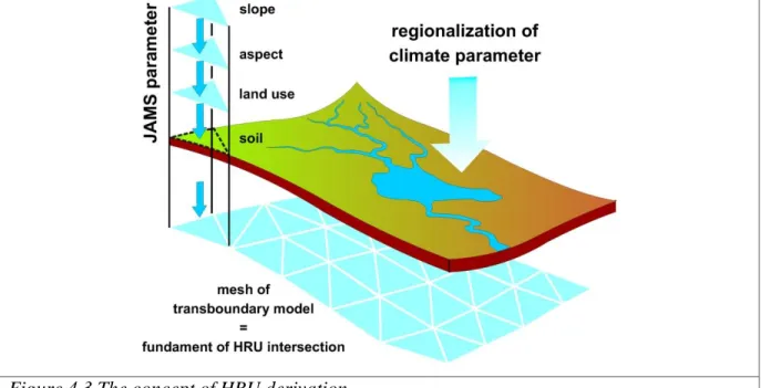
To model Darga catchment we used hydrological response unit and daily time step with a simulation period of 10 years, from 03/01/2003 to 25/12/2012. Hydrological Response Unit (HRU) are homogenous entities delineated by GIS analysis of relevant spatially distributed information (Rödiger et al., 2008), every HRU has unique value of area, elevation, slope, aspect, land-cover and soil type (figure 4.3). For each HRU and each time step climate input are calculate using an inverse-distance-weighting interpolation with optional elevation correction. The process of regionalization has the purpose to switch from punctual values (the measured values available in some stations) to spatially distributed values, one for each model unit (HRU). The steps are the following (from ILMS-Wiki, 2011):
1) Calculation of a linear regression between the station values and the station heights for each time step. Thereby, the Squared Correlation Coefficient (R2) and the slope of the regression line (bH) is calculated.
33
2) Definition of the n gaging stations which are nearest to the particular model unit. The number n which needs to be given during the parameterization is dependent on the density of the station net as well as on the position of the individual stations.
3) Via an Inverse-Distance-Weighted Method (IDW) the weightings of the n stations are defined dependently on their distances for each model unit. Via the IDW-method the horizontal variability of the station data is taken into account according to its spatial position.
4) Calculation of the data value for each model unit with the weightings from point 3 and an optional elevation correction for the consideration of the vertical variability. (The elevation correction is only carried out when the coefficient of determination – calculated under point 1 – goes beyond the threshold of 0.7.)
Figure 4.3 The concept of HRU derivation.
The calculation of the data value for each model unit (DWU) without elevation correction is
carried out with the weightings (W(i)) and the values (MW(i)) of each n gaging station according to:
34
Correction reduces the systematic errors which generally occur in the measurement. For the calculation with elevation correction the elevation difference (HD(i)) between the gauging station and the model unit as well as the slope of the regression line (bH) are taken into
account. Thus, the data value for the model unit (DWU) is calculated according to:
The geographic coordinate system used for the input data was WGS 1984, The World Geodetic System dating from 1984, and the Projected Coordinate System was WGS 1984 – UTM Zone 36N, the Universal Transverse Mercator coordinate system suitable for the area of Israel.
4.2 Model output
The output of the model consist of: runoff, potential and actual evapotranspiration, actual and relative soil moisture, groundwater recharge. The model run autonomously in each model unit and calculates the outputs, then runoff concentration and retention are calculated as summation of the model units to the direct runoff, lateral flow and base flow utilizing the Nash cascade method.
4.2.1 Evapotranspiration
The J2000g model calculates the potential evapotranspiration (PET) using Penman-Monteith equation (Krause and Hanisch 2009; Krause 2002) which is said to be the best adapted evaporation approach due to its physical background (Dunger, 2004). Actual
evapotranspiration (AET) is regarded as the amount of water that evaporates under the constraint of the actual water content of soils; it is calculated as function of potential evapotranspiration and soil moisture by reducing the PET values in relation to the soil moisture budget according to the following function:
35 𝑎𝐸𝑇 = ( 𝑎𝑐𝑡𝑀𝑃𝑆
𝐿𝑖𝑛𝐸𝑇𝑅𝑒𝑑 ∗ 𝑚𝑎𝑥𝑀𝑃𝑆) ∗ 𝑝𝐸𝑇
Where actMPS is actual saturation of MPS (i.e. mid pore storage); maxMPS is the maximal saturation of MPS and LinETRed is a calibration parameters (“linear ET reduction
coefficient”). The maximum saturation of MPS is the volume of the field capacity.
4.2.1.1 Penman-Monteith equation
Evapotranspiration is a component that can be really significant in the study of the water balance. Usually it is not emphasized as it should because it’s hard to verify predictions with direct measurements, which are more affected by uncertainties than other components such as rain and runoff. There are lot of method to estimate evapotranspiration, in this study we have used one of the most popular, the Penman-Monteith equation. It is an equation developed by John Monteith (Monteith, 1965) to estimate the evaporation of water from a surface with vegetation. The equation was derivate by the previous equation of Howard Penman (Penman, 1948), who combined the energy balance with the mass transfer method and derived a method to calculate the evaporation from an open water surface, based on standard climatological values of sunshine, temperature, humidity and wind speed
(www.fao.org). That’s why in its final denomination it has the name of both the scientists. Penman’s equation is the following (Terry, 2004):
λE = ∆ 𝑅𝑛 − 𝐺 + 𝛾𝜆𝐸𝑎 ∆ + 𝛾
where:
- λE is the evaporative latent heat flux
- λ is the latent heat of vaporization (usually a constant value of λ = 2.45 is taken, which is the values at the temperature of 20ºC)
36 - 𝑅𝑛 is net radiation flux
- 𝛾 is the psychrometric constant (0,066) - Ea is the vapor transport flux
- G is the soil heat flux.
From this equation the Penman-Monteith equation was derived, It takes in account particular vegetation parameters such as stomata resistance and leaf area index and include also a bulk surface resistance term. The equation is nowadays used for evapotranspiration calculation by The Food and Agriculture Organization of United Nations (FAO) and The American Society of Civil Engineers, among others. Its formulation, for daily values, is the following (Terry, 2004): λETo = ∆ 𝑅𝑛 − 𝐺 + 86400 𝜌𝑎𝐶𝑃 𝑒𝑠𝑜−𝑒𝑎 𝑟𝑎𝑣 ∆ + 𝛾 1 + 𝑟𝑠 𝑟𝑎𝑣
where the new terms represent: - 𝜌𝑎 is air density,
- 𝐶𝑃is specific heat of dry air,
- 𝑒𝑠𝑜 is mean saturated vapor pressure calculated as the mean 𝑒𝑜 at the daily minimum and maximum air temperature,
- 𝑟𝑎𝑣 is the bulk surface aerodynamic resistance for water vapor, - 𝑒𝑎 is the mean daily ambient vapor pressure,
- 𝑟𝑠 is the canopy surface resistance
The equation take in account parameters that influence, from uniform zone of vegetation, energy exchange and corresponding latent heat flux (evapotranspiration). Most of this values come from measurements or can be calculated from weather data. The result of this equation can also be expressed as the evapotranspiration of a big leaf described by two groups of
37
parameters, one characterized by atmospheric physics and canopy architecture (𝑟𝑎𝑣, 𝑟𝑠 ) and the other one by the biology of the surface (light attenuation, leaf stomatal resistances, etc.) and environmental conditions (irradiance, vapor pressure deficit, etc.).
Bulk surface aerodynamic resistance control the flux of heat and water from the evaporating surface to the air above the canopy according to this equation (Terry, 2004):
𝑟𝑎𝑣 = ln 𝑧𝑤−𝑑 𝑧𝑜𝑚 ln 𝑧𝑟−𝑑 𝑧𝑜𝑣 𝑘2𝑈 𝑧 Where:
- 𝑧𝑤 height of wind measurements - 𝑧𝑟 is height of humidity measurements, - d is zero plane displacement height,
- 𝑧𝑜𝑚 is roughness length governing momentum transfer, - 𝑧𝑜𝑣 is roughness length governing transfer of heat and vapour, - K is the von Karman's constant (0.41),
- 𝑈𝑧 is wind speed at height 𝑧𝑤.
The equation is written for climatic conditions near the adiabatic ones, which means no heat exchange or a really small one, and for long time steps. The use of the equation for short time periods needs the addition of corrections for stability.
Canopy surface resistance describes vapour’s flow resistance through the transpiring surface. Where the soil is not completely covered by vegetation, there is an effect of evaporation from soil surface. Canopy surface resistance is also influenced by the water content of the
vegetation. The following formula is an approximation of the real behavior of that parameter (www.fao.org):
38 𝑟𝑠 =
𝑟𝑙 𝐿𝐴𝐼 Where:
- 𝑟𝑙 is stomatal resistance of the well-illuminated leaf, - LAI is leaf area index.
4.2.2 Soil water budget
The soil water budged is the component of J2000g that distributes the water present in the system, coming from rain and eventually snow, in the different output storage. Water is first send in the evaporation module until the value of potential evapotranspiration is reached. After that the surplus is divided, by some parameters of the model, between runoff and infiltration. Infiltration goes in the soil water storage and from there the excess of water is divided between lateral flow and groundwater recharge. This partition is controlled by slope and a parameter calibrate by the user.
4.2.3 Snow cover
Model can also calculate snow cover in function of two values of temperature: - accumulation temperature, mean between Tmin and Taverage
- Melting temperature, mean between Taverage and Tmax
Based on these values a snow melt factor is calculated. In this study snow module was totally ignored because the occurrence of snow in the area can be disregarded.
39
4.3 Model’s parameters
Parameters of the model have to be configured by the user to make the model prediction fit with observed values in the phase of calibration. All the J2000g parameters are listed and described below, with brief discussion of their control on main hydrological process. InitSoilWater.FCAdaptation: It is the adaption factor which multiplies the absolute pore volume of the soil and defines the water volume which can be stored in the soil component of the model. It controls soil moisture; if the value is high groundwater recharge decreases because less water goes in the ground; actET increase because more water is stored in the soil and can evaporate.
SoilWater.lat.VertDist: it controls if water goes to groundwater recharge or to interflow, if the value is small most of the water goes to the groundwater recharge, if it is higher more water goes to the lateral runoff.
SoilWater.linETRed: Actual ET is calculated as a function of PET and actual soil moisture. The linETred parameter is a reduction coefficient, which directly decreases AET and
therefore increases actual soil moisture. With increasing soil moisture in the model more water is available for all runoff components, including direct runoff (RD1), lateral runoff (RD2) and also percolation (=GWR). As a result, groundwater recharge can partly be increased, by reducing the AET by choosing a larger linEtred factor.
SoilWater.petMult: when this value increases actET also increases and runoff decreases because less water flows in the basin; PetMult increases or decreases the absolute potential evapotranspiration and is therefore an energy balance parameter. Increasing PET values also leads to increasing AET values and therefore to decreasing soil moisture storage in the
model. When less water goes in the soil water storage, all runoff components are affected and have smaller values.
SoilWater.maxPercAdaptation: it controls the maximum percolation (means maximum recharge) per day in mm. When decreasing this value, groundwater recharge is limited and direct and lateral runoff increase. The parameter doesn’t affect actET.
40
Alpha (α): it is the distribution coefficient for the two groundwater components and controls the heavy that the model gives to the fast and slow component of the groundwater; in fact, the model simulates the recharge of an aquifer having double porosity. Low alpha values mean that the prevalent component of the groundwater recharge is the slow one, high values mean that the fast component is the most important one. In this area the dynamic of the recharge is better described by the fast component, so α=0.7 is chosen, which means 70% fast component and 30% slow one.
k1 and k2 are recession parameters to slow down baseflow.
41
5. INPUT DATA
5.1 Meteorological input data
The model needs spatially distributed information about temperature, humidity, precipitation, wind speed and hours of sun, for all the stations available around and in the study area, in order to make the most precise interpolation as possible and obtain spatially distributed inputs for the area. Every station has to be labeled with a name and a unique identification number, and characterized by coordinates and the value of elevation. Series in every station have to be complete for all the period of the model simulation and for all missing values must be coded as -9999.
Meteorological data come from different sources, mostly local authorities such as Israeli Meteorological Service (IMS) and Palestine Meteorological Service (PMS) and, were not enough, satellite data.
As said before not all the time series of every station has to be complete of real values, there can be some missing values (-9999), but it is necessary that for every time step (in our case for every day) there is at least one value available; if not, the interpolation is not possible and the model cannot run in that day (running fails and an error message is shown). If there is only one value available for a day, interpolation is not needed and this value is taken as the one for all the catchment.
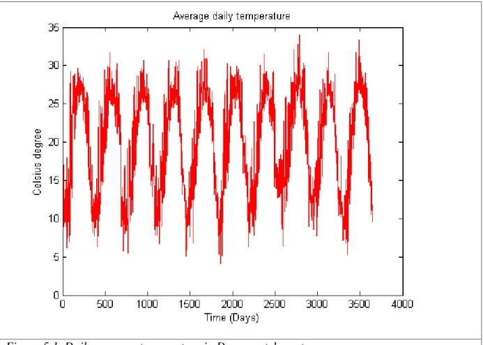
The model requires maximum minimum and average daily temperature values, there are values for 26 stations around and in the catchment; the measure unit is Celsius degree. Daily average temperature is showed in figure 5.1; it ranges from 5 to 35 degree.
42
Figure 5.1. Daily average temperature in Darga catchment.
Concerning humidity the values needed are relative and absolute humidity. Absolute
humidity is the water content of air, indicates the amount of water vapor (g) per unit volume (cm3); its measure unit is g/ cm3. Relative humidity is express as percent, so it has no
measure unit, it range from 0 to 100. For Absolute humidity there are 8 stations with available values, for Relative humidity 13 stations.
Precipitation is one of the most important input variables needed by the model for performing hydrological prediction; we had access to time series collected at 28 stations. For this input we make a further restriction in the chosen of data, to be sure about the quality of the interpolation: for every day the stations with available values are enough to cover an area equal or bigger than the catchment, which means connecting all the stations with values for each day we obtain an area that entirely includes the catchment. In this way we are sure that the distributed input coming from the interpolation is in every time step a good description of the reality because it is generated by an appropriate number of stations, in fact, for every day
43
there are at least three stations available with values (the smallest number of points to make an area). Measure unit is mm. before the simulation punctual values of every station are interpolated by the model in order to provide a distributed trend of the precipitation in the area (figure 5.2)
Figure 5.2. Distributed precipitation coming from the interpolation of measured values from 28 stations surrounding and within the study catchment, the map shows the rainfall depth assigned to each one of the triangular HRU.
Wind speed input requires the daily speed of the wind in m/s, the stations with available time series are 13.
Concerning the hours of sunshine, we used a mix of measured values and satellite values because we had only 2 stations with measured values and the time series were not long enough to entirely cover the run period of the model, so we downloaded a complete time
44
series for the period 2003-2010 from ERA database to complete the missing values (http://www.era-envhealth.eu)
In addition to the meteorological input discussed above, J2000g needs a runoff series in the catchment outlet for comparison purposes; we provided this file to the model, even though all values except for 42 days were missing values.
5.2 Catchment’s input data
Four tables describe the catchment regarding topography, soil, hydro-geology and land use. Each table has to start with “#name of the table” and close with “#end of file”.
The most important table the model needs is called HRU_surface which contain all the information about surface and structure of the catchment (figure 5.3). The model calculates the hydrological output variables in each HRU and for each time step. HRU network in this catchment counts 3160 units and for every time-step calculations will be done for each of this units. In the table each HRU is defined by an ID number (-), the extension of the area (m2), the coordinates of the central point of the HRU area (°, WGS84), elevation (m), slope (°) and aspect (°). Moreover the table contain other three ID (-) which refers to other three tables contain information about soil, land use and hydrogeology.
Figure 5.3. HRU table
45
Hgeo: the table contains the IDs which refer to the ones of the HRU table and for each ID a value of the maximum possible percolation rate per time interval in mm per time unit. This value can also be seen as the maximum ground water recharge can occurs in the geology formation.
Landuse: contains vegetation parameters that are needed for evapotranspiration calculation according to Penman-Monteith equation. For the ID of each land use unit have to correspond:
- a description of the land use (urban, olive, agricultural crop, etc.); - value of albedo (-);
- values of stomata resistances for good water availability (s/m) for the months January to December;
- values of leaf area index (m2/m2) for four Julian days (110, 150, 250, 280) for a terrain height of 400 m above the sea level;
- values of effective vegetation height (m) for the same Julian days as before (110, 150, 250, 280) for a terrain height of 400 m above the sea level;
- value of effective root depth (dm); - Value of sealed degree (%).
Albedo is defined as the ratio of reflected radiation from the surface to incident radiation upon it. Being a dimensionless fraction, it is expressed as a percentage, in a scale from 0 to 1, where 0 means no reflecting power of a perfectly black surface, and 1 means a white surface with perfect reflection power.
Stomata Resistance is the opposition of the stomata of a leaf to the passage of carbon dioxide (CO2) entering, or water vapor exiting through it. Stomata are small pores on the top and
bottom of a leaf that are responsible for taking in and expelling CO2 and moisture from and
to the outside air.
Leaf area index is a variable dimensionless defined as the total one-sided area of green leaves in a vegetation canopy relative to a unit ground area. LAI ignore canopy details such as leaf angle distribution, canopy height or shape.
46
Julian day refers to a continuous count of days from 1 January to 31 December; an integer is assigned to each whole solar day. The four days required by the model are:
- 110 20 April - 150 29 May - 250 6 September - 280 7 October
Sealed degree is a percent number, in a scale from 0 to 1, describing how much the water infiltration is allowed. For example, a road with asphalt doesn’t allow any infiltration so the degree of sealing should be zero.
Soil: the table contains soil-physical parameters for each soil unit that occurs in the catchment:
- SID, integer that represent an unique ID that connects this table to the HRU table - Depth, Depth of the soil (cm)
- Fc_sum, Entire usable field capacity of the soil (mm)
- Fc_1 to fc_n, usable field capacity for each decimeter in mm/dm
Field capacity is a hydrological constant of each soil, definable as the amount of soil moisture or water content held in the soil after excess water has drained away.
47
6. GIS-BASED HYDROLOGICAL ANALYSIS
The aim of this chapter is to describe in a detailed way all the steps to derivate the shape of the catchment and to extract all the useful information from the area that we can obtain making an hydrological analysis with a GIS system. The starting point is the previous knowledge of the digital elevation model (DEM) and the position of the basin’s outlet.
6.1 Management of information in a GIS system
GIS is the acronym of Geographic Information System. GIS environments store, represent and analyze geo-referenced information, which means data whose geographic coordinate are known.
There are two type of data:
- Vector data: graphical geo-referenced objects (points, lines, poligons, etc.).
- Raster data: generally rectangular grids of cells, where each cell is characterized by coordinates and an assigned value.
Vector data can also be divided in three different categories:
- Points: a set of coordinates (x,y) defining a set of points, and each point is linked with a record of information in the database. There is an univocal connection between point and its record.
- Lines: object with the shape of segment whose vertexes are geographically known. Every feature is linked with a record in the database table (table of attributes)
- Polygons: object representing closed area, its vertexes are known and the all area can be linked with some data.
6.2 Basic definitions
Digital elevation model (DEM) is the spatially distribution of altitude in an area, in digital format. It is usually a raster file in which every point is linked with its value of absolute height. (figure 6.1)
48
49
In this study DEM, measurement stations’ coordinates and all the other data loaded in GIS are referenced in the UTM system. The Universal Transverse of Mecator is a projection of the terrestrial surface on a plane, it describes all the world’s surface but North and South poles, in which another projection is used. In UTM system Hearth is divided in 60 time zones, each one 6° longitude large. Moreover it is divided by parallels in 20 “belts” of 8° latitude. The intersection of time zones and “belts” generates zones, every point on the terrestrial surface belong to a zone and is described by unique values of latitude and longitude.
For derivation of the catchment’s shape and the others hydrological characteristics of the study area, we will use the “Hydrologytools” of ArcGis.
6.3 Derivation of Darga catchment’s shape
Calculation of the “Flow Direction”: this function creates a raster with the flow direction of every cell to the downstream one according to the “highest slope” criterion. This means the function simulate the natural direction of fluid’s particle from one cell to the next (figure 6.2). We have to put the DEM file as input.
A perfect “Flow Direction” should contain only 8 values, which represent the 8 cells neighboring in which the water can flow because we are working in a simplified reality where space is divided in square cells. But the first Flow Direction calculated has more than just 8 values, we can observe that looking in the Attribute Table of our file. Some of this values represents sinks, cells in which water can’t flow nowhere because all the neighboring cells have higher altitude. Sinks are depression into the DEM which can represent real topography’s depressions or errors in the data. There a function in ArcGis to identify sinks and correct them if they belong to the second group. We used “Sink” function
(ArcToolbox>Spatial Analyst Tools>Hydrology>Sink): we put Flow Direction raster file as input and obtain the map of sinks in the area (figure 6.3).
50
Figura 6.2 Flow direction. Figure 6.3 Sinks.
The output is a set of black points which represents depressions (figure 6.3) into the DEM. In our case this depressions interrupt somewhere the principal river of the catchment, this is completely in contrast with the definition on catchment because the water cannot flow to the outlet point. So this case depressions have to be filled with the “Fill” function: correction consists in increasing the value of altitude of every sink until it has reached the minimum value of the neighboring cells. The result is a DEM with regular trend. For all the next operations the filled DEM will be used.
First, we need to recalculate a new Flow Direction, utilizing the new DEM. The procedure is exactly the same (already explained above) but the new raster file will contain only the 8 value (figure 6.4): 1, 2, 4, 8, 16, 32, 64 and 128, as explained before.
51
Calculation of “Flow Accumulation”: this function give as output a raster file containing the flux accumulated in every cell counting for each cell the total number of cells drained by that cell.
Figure 6.4 Flow direction with filled DEM.
Flow Accumulation represents the content of water that can flow in every cell, according to this assumptions:
- All the water became surface flow,
- There is no interception, evapotranspiration and loss in soil;
Flow Accumulation can be seen as quantity of rain falling in the area distributed in every cell. Cells with high value of Flow Accumulation are zones of high concentration of water that can belong to rivers, otherwise cells with value of zero are zone of high altitude and can belong to watershed.