BioOne Complete (complete.BioOne.org) is a full-text database of 200 subscribed and open-access titles in the biological, ecological, and environmental sciences published by nonprofit societies, associations, museums, institutions, and presses.
Your use of this PDF, the BioOne Complete website, and all posted and associated content indicates your acceptance of BioOne’s Terms of Use, available at www.bioone.org/terms-of-use.
Usage of BioOne Complete content is strictly limited to personal, educational, and non-commercial use. Commercial inquiries or rights and permissions requests should be directed to the individual publisher as copyright holder.
BioOne sees sustainable scholarly publishing as an inherently collaborative enterprise connecting authors, nonprofit
publishers, academic institutions, research libraries, and research funders in the common goal of maximizing access to critical research.
A new subspecies of Corydalis densiflora (Papaveraceae) from the
Apennines (Italy)
Authors: Fabio Conti, Luca Bracchetti, Dimitar Uzunov, and Fabrizio Bartolucci
Source: Willdenowia, 49(1) : 53-64
Published By: Botanic Garden and Botanical Museum Berlin (BGBM)
URL: https://doi.org/10.3372/wi.49.49107
Willdenowia
Annals of the Botanic Garden and Botanical Museum Berlin
FABIO CONTI1*, LUCA BRACCHETTI2, DIMITAR UZUNOV3 & FABRIZIO BARTOLUCCI1
A new subspecies of Corydalis densiflora (Papaveraceae) from the Apennines (Italy)
Version of record first published online on 29 March 2019 ahead of inclusion in April 2019 issue.
Abstract: A morphometric study of populations from the central-southern Apennines and Sicily of the Italian
en-demic Corydalis densiflora has been undertaken, based on herbarium specimens and field research. A new subspe-cies, C. densiflora subsp. apennina, is described from the central Apennines. It differs from C. densiflora s.str. by its more divided leaves and bracts, basal leaf with more numerous and narrower leaflets, longer middle and lateral lobes of middle and upper bracts, narrower lower petal wing, shorter inner petals and shorter upper stamen.
Key words: Apennines, Corydalis, endemic, Italy, new taxon, Papaveraceae, taxonomy
Article history: Received 17 September 2018; peer-review completed 16 November 2018; received in revised form
30 January 2019; accepted for publication 31 January 2019.
Citation: Conti F., Bracchetti L., Uzunov D. & Bartolucci F. 2019: A new subspecies of Corydalis densiflora (Papa veraceae) from the Apennines (Italy). – Willdenowia 49: 53 – 64. doi: https://doi.org/10.3372/wi.49.49107
Introduction
The genus Corydalis DC. (Papaveraceae) consists of about 440 species distributed in Eurasia, North America and Africa (Lidén & Zetterlund 1997). Corydalis den
siflora C. Presl was described from Sicily “in
nemoro-sis Nebrodum” (Presl & Presl 1822). The name was recently typified based on a specimen housed in PRC (Conti & al. 2015). This taxon was misunderstood by Italian botanists and consequently the understanding of its distribution range was usually incomplete. Fiori (1924) recorded it as C. solida var. densiflora (C. Presl) Boiss. for Trentino-Alto Adige, southern Apennines and Sicily. Pignatti (1982) treated this taxon in a note to the name C. solida, as C. solida var. densiflora, recorded for Calabria and Sicily and not confirmed in Abruzzo.
More recently, Pignatti (2017) recognized two taxa at subspecies level: C. solida (L.) Clairv. subsp. solida and
C. solida subsp. densiflora (C. Presl) Hayek, but
indi-cating erroneous distributions. Corydalis densiflora is currently recognized at species level (Lidén & Zetter-lund 1997; Conti & al. 2014, 2015; Peruzzi & al. 2015; Bartolucci & al. 2018), distinguished from C. solida by several morphological characters (Lidén & Zetterlund 1997; and pers. obs.). It differs by compact racemes (vs loose racemes), bracts as long as wide (vs usually longer than wide), floral pedicels 3 – 8(– 10) mm long (vs 5 – 15 mm long), outer petals narrowly winged (vs broadly winged), corolla apex obtuse to slightly emar-ginate (vs usually emaremar-ginate), lower petal usually without or with a small pouch at base (vs usually with a prominent pouch at base).
1 Scuola di Bioscienze e Medicina Veterinaria, Università di Camerino – Centro Ricerche Floristiche dell’Appennino, Parco Na-zionale del Gran Sasso e Monti della Laga, San Colombo, 67021 Barisciano (L’Aquila), Italy; *e-mail: [email protected] (author for correspondence).
2 Scuola di Bioscienze e Medicina Veterinaria, Università di Camerino, URDIS, Lungomare Scipioni 6, 63074 San Benedetto del Tronto (Ascoli Piceno), Italy.
Corydalis densiflora is endemic to central-southern
Italy and Sicily (Peruzzi & al. 2014, 2015; Bartolucci & al. 2018), occurring in Umbria, Marche, Lazio, Abruzzo, Basilicata, Calabria, Sicily and not confirmed in Molise (Conti & al. 2005, 2015; Del Vico & al. 2014; Bartolucci & al. 2018). However, our preliminary observations on fresh material and the study of herbarium specimens evidenced a certain degree of morphological variability within C. densiflora, seemingly linked to geographical distribution (Conti & al. 2014, 2015).
Material and methods
Plant materialThis study is based mainly on field surveys and an exten-sive analysis of relevant literature, careful examination of herbarium specimens (including the original material) in APP, BC, CAT, CLU, L, LD, MA, MPU, NAP, P, PAL, PRC and UTV (herbarium codes follow Thiers 2018+) and the personal collection of D. Uzunov (Cosenza).
In order to investigate the variability and to clarify the systematics of Corydalis densiflora, about of 15 plants from each of five localities (two from the C Apennines, two from the S Apennines and one from Sicily) were studied.
C Apennines:
L Gran Sasso, Piano Locce (Barisciano), pascoli, 1236 m, 23 Apr 2012, F. Conti & F. Bartolucci V Velino, Monte Fratta (Lucoli), radure e margini di
faggeta, 1600 m, 15 May 2012, F. Conti & F. Barto
lucci
S Apennines:
C Catena Costiera, Passo della Crocetta, 1100 m, 31 Mar 2012, D. Uzunov; ibidem, 17 Apr 2012, D. Uzunov P Pollino, Mormanno, 950 m, 6 May 2012, D. Uzunov Sicily:
M Madonie, Piano Battaglia, 1580 m, 25 Apr 2012, D.
Uzunov
Data acquisition
All plants were scanned before drying, using a flat scan-ner with a resolution of 600 dpi. Firstly, images were acquired from all plants; secondly, the different organs were separated and scanned again with highest resolu-tion in order to capture needed details. All measurements were made by ImageJ software (Rasband 1997 – 2016). This procedure is time saving and allows the acquisition of a large number of characters from fresh plant mate-rial, without the preliminary need of choosing some of them. A total of 72 individuals, scanned before drying, were studied measuring the following quantitative char-acters:
1. number of flowers; 2. number of leaves; 3. length of scale leaf; 4. length of basal leaf; 5. width of basal leaf; 6. number of leaflets of basal leaf; 7. length of petiole of basal leaf; 8. length of middle rachis of basal leaf; 9. length of terminal rachis of basal leaf; 10. length of central leaflet of basal leaf; 11. width of central leaflet of basal leaf; 12. length of basal bract; 13. width of basal bract; 14. number of teeth of basal bract; 15. number of lobes of basal bract; 16. length of middle bract; 17. width of middle bract; 18. length of central lobe of middle bract; 19. width of central lobe of middle bract; 20. length of lateral lobe of middle bract; 21. number of teeth of middle bract; 22. number of lobes of middle bract; 23. length of upper bract; 24. width of upper bract; 25. length of central lobe of upper bract; 26. width of central lobe of upper bract; 27. length of lateral lobe of upper bract; 28. width of lateral lobe of upper bract; 29. sinus depth of lateral lobe of upper bract; 30. number of teeth of upper bract; 31. number of lobes of upper bract; 32. length of pedicel of basal flower; 33. length of pedicel of middle flower; 34. length of pedicel of upper flower; 35. length of flower; 36. maximum width of corolla tube; 37. length of spur; 38. length of upper petal; 39. length of wing of upper petal; 40. length of wing of lower petal; 41. length of lower petal; 42. width of lower petal; 43. length of inner petal; 44. length of ovary; 45. length of upper stamen; 46. width of wing of lower petal.
Statistical analyses
First, descriptive statistics (mean, median and quartiles) and graphs (box plots) were carried out. Then, our data were found to depart from normality, through the Shapiro-Wilk test (Shapiro & Wilk 1965). To understand the similarities (and differences) between the studied populations, univari-ate analysis of variance (one-way ANOVA) and multivari-ate analysis (Principal Component Analysis [PCA] and Discriminant Analysis [DA]) for the studied groups were carried out. Furthermore, in order to detect significant dif-ferences between their averages, the a posteri ori compari-son of each pair of means was performed in ANOVA; this by Tukey’s honestly significant differences (HSD) test. The PCA (Sneath & Sokal 1973; Krzanowski 1990) is an exploratory analysis and in this work was performed to look for the existence of potential patterns. Subsequently, to verify the a priori explicit hypothesis of populations membership, defined on the geographical (central Apen-nines and southern ApenApen-nines [L, V, P] vs southern Ap-ennines and Sicily [C, M]) and morphological basis, the DA (Fisher 1936; Klecka 1980) was used. These analyses were performed using SPSS version 24.0 (IBM 2016) and XLSTAT version 2017.3 (Addinsoft 2017).
Results
Descriptive statistics and one-way ANOVA
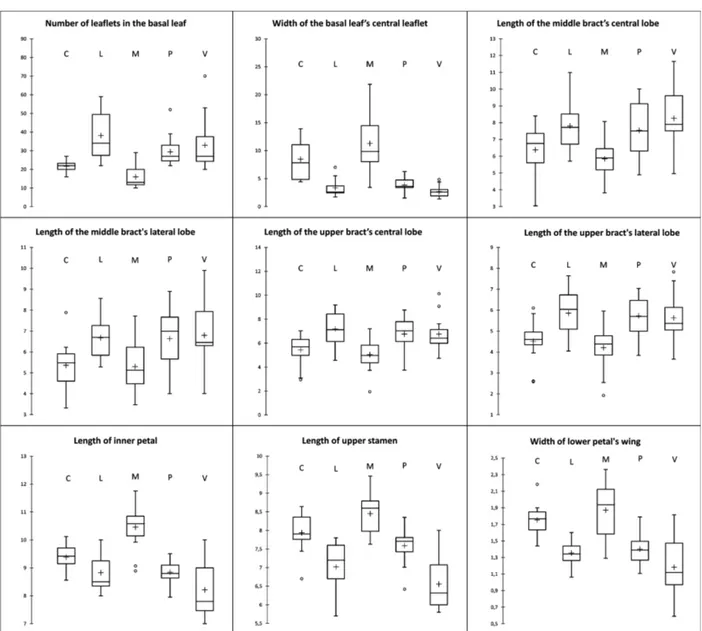
results respectively. Table 2 also shows the groupings based on the similarity of the means (Tukey’s test, HSD) for the studied popula-tions. Of the 46 variables analysed, 30 showed significant differences among the populations (P > 0.05). By the a posteriori test, the differ-entiation between the L-V-P and M-C groups, is defined by nine var-iables (Table 2). Fig. 1 displays the box plot of these variables (number of leaflets of basal leaf; width of central leaflet of basal leaf; length of central lobe of middle bract; length of lateral lobe of middle bract; length of central lobe of up-per bract; length of lateral lobe of upper bract; length of inner petal; length of upper stamen; width of wing of lower petal).
Factorial analysis
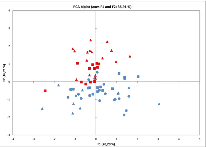
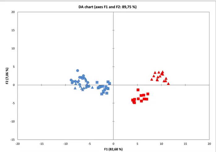
The diversity resulting from PCA analysis is based on the ar-rangement of the first two princi-pal components, which explain 36.91 % of the total variability (F1 = 20.20 %, F2 = 16.71 %). Scores of each specimen on the two prin-cipal components was plotted in PCA bi-plot (Fig. 2), allowing visualization of the positions of the specimens. Mainly on F2, a separation between two groups is observed; for positive values the Madonie and Catena Costiera group is defined, while for nega-tive values the Gran Sasso, Velino and Pollino group is defined. By squared cosines (PCA), the vari-ables that contribute most to define the F1 component are: 16 (0.576), 23 (0.567), 4 (0.541), 13 (0.538), 20 (0.496), 8 (0.450), 5 (0.417) and 27 (0.411). For F2 the varia-bles are: 11 (0.625), 45 (0.569), 43 (0.508), 44 (0.508), 6 (0.388) and 46 (0.337). DA was used in order to verify if the variables allow defi-nition of the studied groups and show as well as possible how sepa-rated they are. The first two axes of DA (Fig. 3) describe 82.68 % and 7.06 %, respectively, and the two box tests (Chi-square and
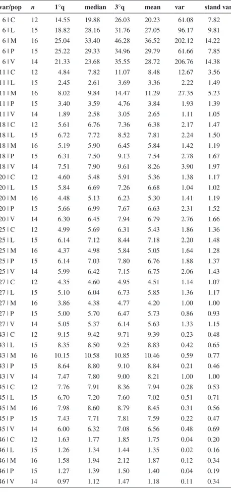
Table 1. Descriptive statistics of variables that differentiate the two groups (L-V-P vs M-C) in ANOVA (var/pop: variable/population; var: variable; n: number of observations; 1°q: first quartile; 3°q: third quartile; stand var: standard variation).
var/pop n 1°q median 3°q mean var stand var
6 | C 12 14.55 19.88 26.03 20.23 61.08 7.82 6 | L 15 18.82 28.16 31.76 27.05 96.17 9.81 6 | M 16 25.04 33.40 46.28 36.52 202.12 14.22 6 | P 15 25.22 29.33 34.96 29.79 61.66 7.85 6 | V 14 21.33 23.68 35.55 28.72 206.76 14.38 11 | C 12 4.84 7.82 11.07 8.48 12.67 3.56 11 | L 15 2.45 2.61 3.69 3.36 2.22 1.49 11 | M 16 8.02 9.84 14.47 11.29 27.35 5.23 11 | P 15 3.40 3.59 4.76 3.84 1.93 1.39 11 | V 14 1.89 2.58 3.05 2.65 1.11 1.05 18 | C 12 5.61 6.76 7.36 6.38 2.17 1.47 18 | L 15 6.72 7.72 8.52 7.81 2.24 1.50 18 | M 16 5.19 5.90 6.45 5.84 1.42 1.19 18 | P 15 6.31 7.50 9.13 7.54 2.78 1.67 18 | V 14 7.51 7.90 9.61 8.26 3.90 1.97 20 | C 12 4.60 5.48 5.91 5.36 1.38 1.17 20 | L 15 5.84 6.69 7.26 6.68 1.04 1.02 20 | M 16 4.48 5.13 6.23 5.30 1.41 1.19 20 | P 15 5.66 6.99 7.67 6.63 2.31 1.52 20 | V 14 6.30 6.45 7.94 6.79 2.76 1.66 25 | C 12 4.99 5.69 6.31 5.43 1.86 1.36 25 | L 15 6.14 7.12 8.44 7.18 2.20 1.48 25 | M 16 4.37 4.98 5.84 5.05 1.64 1.28 25 | P 15 6.14 7.03 7.80 6.76 1.88 1.37 25 | V 14 5.99 6.42 7.15 6.75 2.06 1.43 27 | C 12 4.35 4.60 4.95 4.51 1.14 1.07 27 | L 15 5.10 6.04 6.73 5.85 1.36 1.17 27 | M 16 3.86 4.38 4.77 4.20 1.00 1.00 27 | P 15 5.00 5.70 6.47 5.73 0.86 0.93 27 | V 14 5.05 5.37 6.14 5.63 1.33 1.15 43 | C 12 9.15 9.42 9.71 9.39 0.23 0.48 43 | L 15 8.35 8.50 9.25 8.83 0.42 0.65 43 | M 16 10.15 10.58 10.85 10.46 0.59 0.77 43 | P 15 8.64 8.80 9.10 8.84 0.21 0.46 43 | V 14 7.47 7.80 9.00 8.21 1.00 1.00 45 | C 12 7.76 7.91 8.36 7.94 0.28 0.53 45 | L 15 6.70 7.20 7.60 7.02 0.51 0.71 45 | M 16 7.98 8.60 8.79 8.45 0.31 0.56 45 | P 15 7.43 7.71 7.81 7.59 0.22 0.47 45 | V 14 6.00 6.32 7.08 6.56 0.48 0.69 46 | C 12 1.63 1.77 1.85 1.75 0.04 0.20 46 | L 15 1.26 1.34 1.44 1.35 0.02 0.16 46 | M 16 1.58 1.94 2.12 1.87 0.12 0.34 46 | P 15 1.27 1.39 1.50 1.40 0.04 0.19 46 | V 14 0.97 1.12 1.47 1.18 0.11 0.34
Fischer F) and Kullback’s test confirm that the need to reject the hypothesis that the covariance matrices are equal among the five populations (p-value <0.0001). The correlation indices between variables and factors (Table 3) show that the variability of the first factor is more correlated with the following variables: 11. width of central leaflet of basal leaf (0.72); 43. length of inner petal (0.7); 45. length of upper sta-men (0.72); 46. width of wing of lower petal (0.7). Instead, for the second factor, the most important variables are: 4. length of scale leaf (0.609); 7. length of petiole of basal leaf (0.391). The two-dimensional chart in Fig. 3 repre-sents the observations on the fac-tor axes 1 and 2, extracted from the original explanatory variables by DA. It shows that, in the five studied populations, the group L-V-P (central and southern Ap-ennines) is well defined from the group M-C (southern Apennines and Sicily). The observations of the first group ( L-V-P) are in fact concentrated on the left of the graph, while the second group (M-C) is on the right; essentially, the factor (F1) contributes to this differentiation. The confusion ma-trices of validation are displayed in Table 4.
Discussion
The univariate and multivariate analyses carried out with different techniques (ANOVA, and PCA and DA, respectively) enabled the identification of the existing dif-ferentiation model between the populations of central and ern Apennines (L-V-P) and south-ern Apennines and Sicily (M-C) and to define the variables that characterize it. From a graphical visual approach (PCA and DA graph and box plot), it is easy to observe two well-distinguished systematic groups. The great-est contribution to this diversity
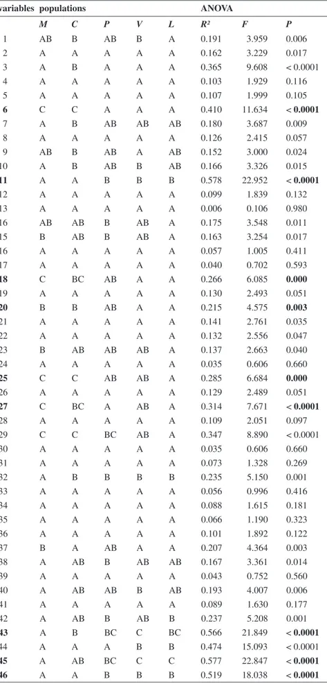
Table 2. Results of ANOVA and populations meberschip based on Tukey’s test (HSD). In
bold the variabilities that differentiate the groups M-C vs L-V-P. variables populations ANOVA
M C P V L R² F P 1 AB B AB B A 0.191 3.959 0.006 2 A A A A A 0.162 3.229 0.017 3 A B A A A 0.365 9.608 < 0.0001 4 A A A A A 0.103 1.929 0.116 5 A A A A A 0.107 1.999 0.105 6 C C A A A 0.410 11.634 < 0.0001 7 A B AB AB AB 0.180 3.687 0.009 8 A A A A A 0.126 2.415 0.057 9 AB B AB A AB 0.152 3.000 0.024 10 A B AB B AB 0.166 3.326 0.015 11 A A B B B 0.578 22.952 < 0.0001 12 A A A A A 0.099 1.839 0.132 13 A A A A A 0.006 0.106 0.980 16 AB AB B AB A 0.175 3.548 0.011 15 B AB B AB A 0.163 3.254 0.017 16 A A A A A 0.057 1.005 0.411 17 A A A A A 0.040 0.702 0.593 18 C BC AB A A 0.266 6.085 0.000 19 A A A A A 0.130 2.493 0.051 20 B B AB A A 0.215 4.575 0.003 21 A A A A A 0.141 2.761 0.035 22 A A A A A 0.132 2.556 0.047 23 B AB AB AB A 0.137 2.663 0.040 24 A A A A A 0.035 0.606 0.660 25 C C AB AB A 0.285 6.684 0.000 26 A A A A A 0.129 2.489 0.051 27 C BC A AB A 0.314 7.671 < 0.0001 28 A A A A A 0.109 2.051 0.097 29 C C BC AB A 0.347 8.890 < 0.0001 30 A A A A A 0.035 0.606 0.660 31 A A A A A 0.073 1.328 0.269 32 A B B B B 0.235 5.150 0.001 33 A A A A A 0.056 0.996 0.416 34 A A A A A 0.088 1.615 0.181 35 A A A A A 0.066 1.190 0.323 36 A A A A A 0.101 1.892 0.122 37 B A AB A A 0.207 4.364 0.003 38 A AB B AB AB 0.167 3.361 0.014 39 A A A A A 0.043 0.752 0.560 40 A AB AB B AB 0.193 4.007 0.006 41 A A A A A 0.089 1.630 0.177 42 A AB B AB B 0.237 5.208 0.001 43 A B BC C BC 0.566 21.849 < 0.0001 44 A A A B B 0.474 15.093 < 0.0001 45 A AB BC C C 0.577 22.847 < 0.0001 46 A A B B B 0.519 18.038 < 0.0001
comes from shape of leaves and bracts and from few flower features such as length of inner petals and upper stamen and width of wing of lower petal. Noteworthy is the poor overlapping of the M and C observations, which however are far from the L-V-P group from which they differ; this aspect could be a starting point for a future investigation.
Taxonomic treatment
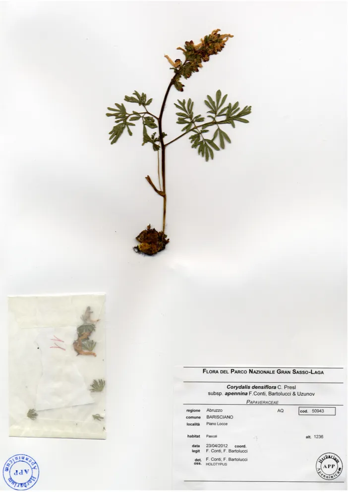
Corydalis densiflora subsp. apennina F. Conti, Bartolucci & Uzunov, subsp. nov. – Fig. 4, 5, 6.
Holotype: Italy, Abruzzo, Barisciano (L’Aquila), Gran Sas-so, in località Piano Locce, pascoli, 1236 m, 23 Apr 2012,
Conti & Bartolucci (APP no. 50943 [Fig. 5]; isotypes: APP
nos. 50938, 50939, 50940, 50941, 50942, 50944, 50945, 50946, 50947, 50948, 51578, 51579, 51580, 51581).
Diagnosis — Corydalis densiflora subsp. apennina
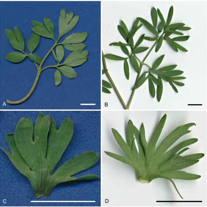
dif-fers from subsp. densiflora by its more divided leaves and bracts (Fig. 6), basal leaf with more numerous leaf-lets (20 –)33.5(– 70) vs (10 –)18.43(– 29), narrower cen-tral leaflet of the basal leaf (1.4 –)3.3(– 7) mm wide vs (3.4 –)10.1(– 21.9) mm wide, longer middle and lateral lobes of the bracts, shorter inner petals (7 –)8.6(– 10) mm long vs (8.6 –)10(– 11.7) mm long, shorter upper stamen, and narrower wing of the lower petal (0.6 –)1.3(– 1.8) mm wide vs (1.3 –)1.8(– 2.4) mm wide.
Description — Stem (4 –)16(– 26) cm tall. Scale leaf
(11.2 –)19.2(– 32.4) mm long. Leaves (2 –)2.5(– 4), alter-nate, usually triternate; leaflets narrowly obovate. Basal leaf (29.5 –)76.4(– 149) mm long × (14 –)54.4(– 91.3) mm wide, with (20 –)33.5(– 70) leaflets; central leaflet (9 –) 17.7(– 26.7) mm long × (1.4 –)3.3(– 7) mm wide; pe tiole (12.1 –)28.5(– 59.2) mm long. Raceme (Fig. 4) usually dense, with (2 –)8.9(– 20) flowers. Bracts slightly wider than long, divided into usually dentate segments. Basal bract (6.9 –)12.3(– 19.1) mm long × (8.9 –)15.9(– 21.5) mm
wide. Middle bract: central lobe (4.9–)7.9(–11.6) mm long × (0.5 –)1.5(– 2.6) mm wide; lateral lobe (4 –)6.7(– 9.9) mm long. Flowers (13.1 –)18.3(– 22.3) mm long; pedicel 1 – 10 mm long. Corolla whitish to pale pink with red mar-gin; maximum width of corolla tube (3.1 –)4.1(– 5.6) mm. Spur (6.9 –)10.4(– 13.5) mm long. Upper petal (7.2 –)8.5(– 9.8) mm long; wing (2.5 –)3.7(– 5.2) mm long. Lower petal (8.2 –)10(– 11.8) mm long × (2.8 –)4.1(– 5.1) mm wide; wing (2.6 –)4.3(– 5.8) mm long × (0.6 –)1.3(– 1.8) mm wide. Inner petals (7 –)8.6(– 10) mm long. Ovary (6.5 –)8.1(– 11) mm long. Upper stamen (5.7 –)7.1(– 8.3) mm long. Fruiting pedicels (1.9 –)3.4(– 6) mm long. Fruits (7.5 –)12.5(– 17.4) mm long × (1.5 –)4.1(– 6.1) mm wide.
Phenology — Flowering from the second half of April to
June, fruiting from May to June.
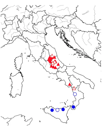
Distribution — Corydalis densiflora subsp. apennina is
endemic to the central and southern Apennines, wide-spread in Umbria, Marche, Lazio, Abruzzo, Campania, Calabria and not confirmed in Molise. The record of
C. solida subsp. solida for Campania (Bartolucci & al.
2018) has to be referred to C. densiflora subsp. apennina.
Corydalis densiflora subsp. densiflora is endemic to
Ca-labria and Sicily (Fig. 7).
Table 3. Variables (Var) / factors (F1, F2) correlations.
Var F1 F2 Var F1 F2 1 -0.076 0.289 24 -0.028 -0.166 2 0.080 0.285 25 -0.527 0.024 3 -0.227 0.609 26 0.195 -0.257 4 -0.036 0.288 27 -0.546 0.003 5 0.137 0.243 28 -0.537 0.230 6 -0.637 0.020 29 0.276 -0.203 7 0.139 0.391 30 0.120 0.140 8 0.042 0.189 31 -0.007 0.018 9 -0.340 0.154 32 0.349 0.335 10 0.189 0.340 33 0.151 0.196 11 0.752 0.103 34 -0.089 0.064 12 0.250 0.158 35 -0.103 -0.041 13 0.074 -0.029 36 0.092 0.270 14 -0.135 0.016 37 -0.297 -0.348 15 -0.294 0.068 38 0.292 0.263 16 -0.216 -0.069 39 0.160 0.013 17 -0.130 -0.050 40 0.292 0.013 18 -0.511 -0.028 41 0.279 0.284 19 0.218 -0.208 42 0.395 0.083 20 -0.450 0.042 43 0.701 0.270 21 0.104 0.066 44 0.639 0.051 22 -0.282 -0.042 45 0.726 0.047 23 -0.361 -0.009 46 0.703 0.021 Fig. 2. Principal Component Analysis (PCA) of all variables. Blue square: P (Pollino); blue triangle: V (Monte Fratta, Velino); blue circle: L (Piano Locce, Gran Sasso); red square: C (Catena Costiera); red triangle: M (Madonie).
Habitat — Meadows, edge and clearings of Fagus syl vatica forest.
Conservation status — According to IUCN criteria
(IUCN Standards and Petitions Subcommittee 2017), we propose to include Corydalis densiflora subsp. apennina in the following category: Least Concern (LC). Recently, Orsenigo & al. (2018) proposed to include C. densiflora at species level in the category LC.
Etymology — The subspecific epithet apennina is an
ad-jective derived from the Apennines.
Identification key to the subspecies of Corydalis
densi-flora
1. Basal leaf with (10 –)18.43(– 29) leaflets, cen-tral leaflet (3.4 –)10.1(– 21.9) mm wide; inner pet-als (8.6 –)10(– 11.7) mm long; wing of lower petal (1.3 –)1.8(– 2.4) mm wide . . . . . . . .C. densiflora subsp. densiflora – Basal leaf with (20 –)33.5(– 70) leaflets, central leaflet
(1.4 –)3.3(– 7) mm wide; inner petals (7 –)8.6(– 10) mm long; wing of lower petal (0.6 –)1.3(– 1.8) mm wide . . . C. densiflora subsp. apennina
Additional specimens studied
Corydalis densiflora subsp. densiflora — Sicilia [Si-cily]: Madonie, Pizzo Carbonara (Palermo), 413836E, 4194461N, UTM-ED50, margine faggeta, 1850 m, 4 Jun 2010, F. Conti, F. Bartolucci & N. Ranalli (APP no. 51529); Madonie, Pizzo Carbonara, 3 May 1992, Brullo
& al. (CAT no. 30332 [digital photo]); ibidem, 9 Jun 1983, S. Brullo (CAT no. 46763 [digital photo]); ibidem, 5 Jun
1990, Brullo & al. (CAT no. 46764 [digital photo]); Ma-donie, Quacella, 3 May 1987, S. Brullo & al. (CAT no. 46761 [digital photo]); Madonie, Piano Battaglia, 27 Apr 1983, S. Brullo (CAT no. 46762 [digital photo]); Mado-nie: faggeta di Battaglia, 37°52'N, 14°02'E, organic moist soil, 1500 – 1600 m, 5 Jun 1990, 1240 Optima Iter Medi-terraneum III in Sicily, Raimondo & al. (PAL); Madonie, Portella Colle, Madonie, 25 Apr 1991, S. Brullo & G.
Spampinato (CAT no. 46765 [digital photo]); Monte Soro,
26 Apr 1981, S. Brullo (CAT no. 46766 [digital photo]); ibidem, 28 May 1982, S. Brullo (CAT no. 46767 [digital photo]); Nebrodi, da Piano Menta a Piano Daini, 19 Apr 1988, S. Brullo & P. Minissale (CAT no. 46768 [digital photo]); Madonie, Piano Battaglia, 1580 m, 25 Apr 2012,
D. Uzunov (herb. Uzunov); Busambra, s.d., Todaro (PAL);
Ficuzza alle Neviere, 8 Apr 1904, A. Terracciano (PAL). — Cala bria: Aspromonte, loc. umbrosis in jugo,
Mon-Fig. 3. Discriminant Analysis (DA) of all variables. Blue square: P (Pollino); blue triangle: V (Monte Fratta, Velino); blue circle: L (Piano Locce, Gran Sasso); red square: C (Catena Costiera); red triangle: M (Madonie).
talto, sol. granit., 1950 – 1956 m, 30 May 1877, 324 ex iti-nere italico III, Huter, Porta & Rigo (P); Catena Costiera, Passo della Crocetta, ad un’altitudine di 1100 m, 31 Mar 2012, D. Uzunov (herb. Uzunov); ibidem, 17 Apr 2012, D.
Uzunov (herb. Uzunov).
Corydalis densiflora subsp. apennina — Marche: Monte Sibilla, presso il Rifugio Sibilla (Montemonaco, Ascoli Piceno), prati, 1600 m, 4 May 2012, F. Conti (APP no. 52556, 52557, 52558, 52559, 52560, 52561, 52562, 52563, 52564, 52565, 52566); M. Macchialta versante NO (Arquata del Tronto), pascolo, suolo calcareo, 1575 m, 4 May 2012, F. Falcinelli (APP no. 57152). — Umbria: La Montagnola versante O (Cascia, Perugia), orlo di faggeta, suolo calcareo, 1295 m, 18 Apr 2012, F. Falcinelli (APP no. 57178); M. la Pelosa versante O-NO (Polino, Terni), orlo di faggeta, suolo calcareo, 1490 m, 23 Apr 2012, F.
Falcinelli (APP no. 57158); M.ti Sibillini, M. Calarelle
versante N-NE (Norcia, Perugia), pascolo, suolo calca-reo, 1530 m, 29 Apr 2012, F. Falcinelli (APP no. 57183); M.ti Sibillini, M. Serra versante SE (Norcia, Perugia), pascolo, suolo calcareo, 1670 – 1685 m, 17 May 2012, F.
Falcinelli (APP no. 57184); M. Maggio, versante E
(Ca-scia, Perugia), orlo di faggeta, suolo calcareo, 1410 m, 21 Apr 2016, F. Falcinelli (APP); M. Maggio, versante NO (Gualdo Tadino, Perugia), orlo di faggeta, suolo calcareo, 1400 m, 21 Apr 2016, F. Falcinelli (APP); Colle del Se-gretario, versante NO (Monteleone Di Spoleto, Perugia), 1305 m, 19 Apr 2016, F. Falcinelli (APP); M. Carpena-le, versante N (Poggiodomo, Perugia), pascolo, 1365 m, 15 Apr 2016, F. Falcinelli (APP); M. Carpenale, versante NO-N (Poggiodomo, Perugia), pascolo, 1335 m, 15 Apr 2016, F. Falcinelli (APP). — Lazio: M. Corno versante E-SE (Leonessa, Rieti), pascolo, suolo calcareo, 1680 m, 9 May 2014, F. Falcinelli (APP no. 57156); M. la Pelosa versante SE (Leonessa, Rieti), orlo di fag geta, suolo calca-reo, 1625 m, 23 Apr 2012, F. Falcinelli (APP no. 57153); ibidem, pascolo ricco, suolo calcareo, 1440 m, 23 Apr 2012, F. Falcinelli (APP no. 57155); M. la Pelosa versante SE (Leonessa, Rieti), pascolo, suolo calcareo, 1570 m, 23 Apr 2012, F. Falcinelli (APP no. 57154); M. Terminillo versante SE (Micigliano), prato comune, 1640 – 1680 m, 12 Jun 2014, F. Falcinelli (APP no. 57157); M. Boragine, Forca di Fao, sentiero 472, M. Arcione–M. Boragine (Cit-tareale, Rieti), 4718498N, 345676E, WGS84 33T, pascoli secondari, 1619 – 1809 m, 15 Apr 2016, F. Conti (APP no. 57369, 57374, 57375); Monti Simbruini al Campo della Pietra e sul M. Autore (Roma), faggete e radure, 1400 m, 2 May 1990, D. Arcioni (FI); Montagne della Duchessa (Rieti), al M. Nuria, 1600 m, in faggeta, 14 May 1989,
D. Arcioni (FI); Monti Reatini al M. Terminillo (Rieti), in
località Pian de’ Valli, c. 1500 m, in faggete e radure, 28 Apr 1989, D. Arcioni (FI); M. Pozzoni, Cittareale (Rie-ti), faggeta, radura, c. 1700 m, 1 May 2010, E. Lattanzi (UTV no. 32032); salendo da Selvarotonda verso Forca di Fao, Cittareale (Rieti), Staz. 7, su cotico erboso al margine di faggeta, 15 Apr 2016, A. Scoppola (UTV no. 36088).
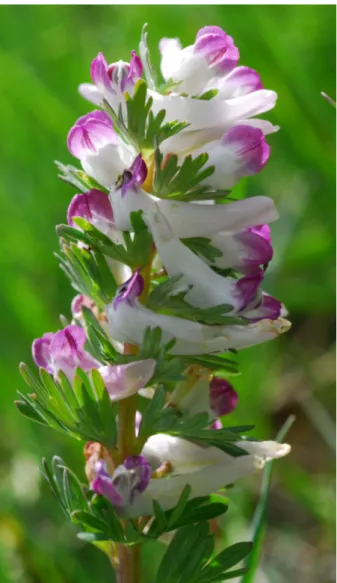
Fig. 4. Flowering raceme of Corydalis densiflora subsp. apen
nina at the type locality, 23 Apr 2012, photographed by F. Conti.
Table 4. Confusion matrices for estimation (above) and for cross-validation results (below) (DA).
from / to C L M P V total % correct
C 12 0 0 0 0 12 100.00 % L 0 15 0 0 0 15 100.00 % M 0 0 16 0 0 16 100.00 % P 0 0 0 15 0 15 100.00 % V 0 0 0 0 14 14 100.00 % total 12 15 16 15 14 72 100.00 %
from / to C L M P V total % correct
C 11 0 1 0 0 12 91.67 % L 0 7 0 1 7 15 46.67 % M 6 4 3 3 0 16 18.75 % P 0 2 0 8 5 15 53.33 % V 0 1 0 1 12 14 85.71 % total 17 14 4 13 24 72 56.94 %
— Abruzzo: Campo Imperatore tra Fonte Cupa e lo Scoppaturo (Castel del Monte, L’Aquila), 42°24.357'N, 13°44.589'E, UTM-ED50, pascoli, 1498 m, 1 May 2003,
F. Conti & D. Tinti (APP no. 9640); Lago Racollo (S.
Stefano di Sessanio, L’Aquila), pascoli, 1550 m, 13 May 2004, D. Tinti (APP no. 10591); Lago di Passane-ta (Barisciano, L’Aquila), pascoli secondari, 1561 m, 18 May 2004, A. Bernardini & L. Morelli (APP no. 14873); base brecciaio del M Puzzillo (Lucoli, L’Aquila), pa-scoli, 1682 m, 17 Jun 2006, F. Conti & R. Soldati (APP no. 30101); M. Puzzillo-Valle Leona (Lucoli, L’Aquila), pascoli, 1500 – 1700 m, 13 Jun 1999, F. Conti (APP no. 30103); Lago S. Pietro (Calascio, L’Aquila), 20 May 2011,
F. Bartolucci (APP no. 46539); sopra Civita d’Antino
ver-so Collelongo (Civita D’antino, L’Aquila), 1540 m, 28 Apr
2010, F. Conti & N. Ranalli (APP no. 49098); Lago di Ba-risciano (BaBa-risciano, L’Aquila), pascoli, 1600 m, 5 May 2012, F. Conti (APP no. 50932); Monte Fratta (Lucoli), radure e margine faggeta, 1600 m, 15 May 2012, F. Conti
& F. Bartolucci (APP no. 52567, 52568, 52569, 52570,
52571, 52572, 52573, 52574, 52575, 52576, 52577, 52578, 52579, 52580, 52581, 52582); Pescasseroli (L’Aquila), Val Cervara, Fondovalle umido, al margine di faggeta, 12 May 2012, A. Scoppola (UTV no. 30730); Monte Rapina, Ca-ramanico Terme (Pescara), prateria montana, 1457 m, 29 Apr 2018, S. Nelli (UTV no. 36596); Monte dei Fiori, pa-scoli, 1550 m, 29 Apr 2018, F. Bartolucci & V. Impiccini (APP). — Campania: Cervati, versante S, 21 May 1987,
M. Buonanno, R. Cerri & A. Santangelo (NAP); Cervati,
versante S, 1800 m, 2 Jun 1987, M. Buonanno, R. Cerri
Fig. 6. A, C: Corydalis densiflora subsp. densiflora from Piano Battaglia (Madonie); B, D: Corydalis densiflora subsp. apennina from Monte Fratta (Velino); A, B: basal leaves; C, D: basal bracts. Scale bars: A – D = 1 cm.
& A. Santangelo (NAP); Cervati, altopiano
di vetta, 6 May 1993, A. Santangelo (NAP). — Calabria: Pollino, Mormanno, 950 m, 6 May 2012, D. Uzunov (herb. Uzunov).
Acknowledgements
Many thanks are due the directors and cu-rators of the consulted herbaria. We wish to thank our friends and colleagues: Fran-cesco Falcinelli, who provided us many specimens of the new taxon from Umbria, and Anna Scoppola, Annalisa Santangelo and Leonardo Gubellini, who provided us with distributional data. We also thank Ås-lög Dahl (GB) and Lorenzo Peruzzi (PI) for their comments on an earlier version of this paper.
References
Addinsoft 2017: XLSTAT: data analysis and statistical solution for Microsoft Excel. – Paris: Addinsoft.
Bartolucci F., Peruzzi L., Galasso G., Alba-no A., Alessandrini A., Ardenghi N. M. G., Astuti G., Bacchetta G., Ballelli S., Banfi E., Barberis G., Bernardo L., Bou-vet D., Bovio M., Cecchi L., Di Pietro R., Domina G., Fascetti S., Fenu G., Festi F., Foggi B., Gallo L., Gottschlich G., Gubellini L., Iamonico D.,
Iberi-te M., Jiménez- Mejías P., Lattanzi E., Marchetti D. Martinetto E., Masin R. R., Medagli P., Passalacqua N. G., Peccenini S., Pennesi R., Pierini B., Poldini L., Prosser F., Raimondo F. M., Roma- Marzio F., Rosati L., Santangelo A., Scoppola A., Scortegagna S., Selvaggi A., Selvi F., Soldano A., Stinca A., Wagen-sommer R. P., Wilhalm T. & Conti F. 2018: An updated checklist of the vascular flora native to Italy. – Pl. Bio-systems 152: 179 – 303.
Conti F., Abbate G., Alessandrini A. & Blasi C. (ed.) 2005: An annotated checklist of the Italian vascular flora. – Roma: Palombi Editori.
Conti F., Bartolucci F., Ceci L. & Uzunov D. 2014: Con-siderazioni sistematiche e tassonomiche su Corydalis
densiflora (Papaveraceae). – Pp. 41 – 42 in: Peruzzi L.
& Domina G. (ed.), Riunione scientifica del Gruppo per la Floristica, Sistematica ed Evoluzione, Società Botanica Italiana, 21 – 22 Nov 2014. – Roma: Società Botanica Italiana.
Conti F., Uzunov D. & Bartolucci F. 2015: Correction of the typification of Corydalis solida var. bracteosa and lectotypification of C. densiflora (Papavera ceae). – Phytotaxa 197: 222 – 224.
Del Vico E., Lattanzi E., Marignani M. & Rosati L. 2014: Specie rare e di interesse conservazionistico di un set-tore poco conosciuto dell’Appennino centrale (Citta-reale, Rieti). – Pp. 33 – 34 in: Peruzzi L. & Domina G. (ed.), Riunione scientifica del Gruppo per la Floristica, Sistematica ed Evoluzione, Società Botanica Italiana, 21 – 22 Nov 2014. – Roma Società Botanica Italiana. Fiori A. 1924: Nuova flora analitica d’Italia 1. – Firenze:
Tip. Ricci.
Fisher R. A. 1936: The use of multiple measurements in taxonomic problems. – Ann. Eugenics 7: 179 – 188. IBM Corp. Released 2016: IBM SPSS statistics for
Win-dows, Version 24.0. – Armonk: IBM Corp.
IUCN Standards and Petitions Subcommittee 2017: Guidelines for using the IUCN Red List categories and criteria. Version 13. Prepared by the Standards and Petitions Subcommittee of the IUCN Species Survival Commission. – Published at http://www .iucn redlist.org/documents/RedListGuidelines.pdf [accessed 3 Apr 2018].
Klecka W. R. 1980: Discriminant analysis. – Sage Uni-versity Papers, Series: Quantitative Application in the Social Sciences 19: 7 – 63.
Fig. 7. Distribution map of Corydalis densiflora subsp. densiflora (blue cir-cles) and C. densiflora subsp. apennina (red triangles) according to the material studied: hollow symbols indicate the populations included in the morphometric study; solid symbols refer to the specimens seen but not used for statistical analyses.
Willdenowia
Open-access online edition bioone.org/journals/willdenowia
Online ISSN 1868-6397 · Print ISSN 0511-9618 · Impact factor 1.500
Published by the Botanic Garden and Botanical Museum Berlin, Freie Universität Berlin © 2019 The Authors · This open-access article is distributed under the CC BY 4.0 licence Krzanowski W. J. 1990: Principles of multivariate
analy-sis. – Oxford: Clarendon Press.
Lidén M. & Zetterlund H. 1997: Corydalis: a gardener’s guide and a monograph of the tuberous species. – Worcestershire: AGS publication Ltd.
Orsenigo S., Montagnani C., Fenu G., Gargano D., Peruzzi L., Abeli T., Alessandrini A., Bacchetta G., Bartolucci F., Bovio M., Brullo C., Brullo S., Car-ta A., Castello M., Cogoni D., Conti F., Domina G., Foggi B., Gennai M., Gigante D., Iberite M., Lasen C., Magrini S., Perrino E., Prosser F., Santange-lo A., Selvaggi A., Stinca A., Vagge I., Villani M., Wagensommer R. P., Wilhalm T., Tartaglini N., Duprè E., Blasi C. & Rossi G. 2018: Red Listing plants un-der full national responsibility: extinction risk and threats in the vascular flora endemic to Italy. – Biol. Conservation 224: 213 – 222.
Peruzzi L., Conti F. & Bartolucci F. 2014: An inventory of vascular plants endemic to Italy. – Phytotaxa 168: 1 – 75.
Peruzzi L., Domina G., Bartolucci F., Galasso G., Pecce-nini S., Raimondo F. M., Albano A., Alessandrini A., Banfi E., Barberis G., Bernardo L., Bovio M., Brullo S., Brundu G., Brunu A., Camarda I., Carta L., Conti F., Croce A., Iamonico D., Iberite M., Iiriti G., Longo
D., Marsili S., Medagli P., Pistarino A., Salmeri C., Santangelo A., Scassellati E., Selvi F., Soldano A., Stinca A., Villani M, Wagen sommer R. P. & Passa-lacqua N. G. 2015: An inventory of the names of vas-cular plants endemic to Italy, their loci classici and types. – Phytotaxa 196: 1 – 217.
Pignatti S. 1982: Flora d’Italia 1. – Bologna: Edagricole. Pignatti S. 2017: Flora d’Italia 1, ed. 2. – Bologna:
Eda-gricole.
Presl J. S. & Presl C. B. (ed.) 1822: Deliciae pragenses, historiam naturalem spectantes. – Pragae: Calve. Rasband W. S. 1997 – 2016: ImageJ – Bethesda: U.S.
National Institutes of Health. – Published at http:// imagej.nih.gov/ij/
Shapiro S. & Wilk M. B. 1965: An analysis of variance test for normality (complete samples). – Biometrika
52: 591 – 611.
Sneath P. H. A. & Sokal R. R. 1973: Numerical taxono-my. Principles and practice of numerical classifica-tion. – San Francisco: W. H. Freeman and Company. Thiers B. 2018+ [continuously updated]: Index
herbari-orum: a global directory of public herbaria and as-sociated staff. New York Botanical Garden’s virtual herbarium. – Published at http://sweetgum.nybg.org /science/ih/ [accessed 30 Apr 2018].