ONE-DIMENSIONAL HYDRODYNAMIC MODELS IN RIVER RESOURCE MANAGEMENT AND POLICY DESIGN

(1)

Università degli Studi di Ferrara

DOTTORATO DI RICERCA IN

SCIENZE DELL’INGEGNERIA

CICLO XXVII

COORDINATORE Prof. Stefano TRILLO

ONE-DIMENSIONAL HYDRODYNAMIC MODELS

IN RIVER RESOURCE MANAGEMENT

AND POLICY DESIGN

Settore Scientifico Disciplinare ICAR/01

Dottorando

Tutore

Dott. Bernardi Dario

Prof. Schippa Leonardo

(2)

(3)

Doctoral thesis in Engineering Science, XXVII cycle – Bernardi Dario

Department of Engineering, University of Ferrara – Italy Supervisor: Dr. Leonardo Schippa, PhD, LPE

Università degli Studi di Ferrara Ferrara, April 10th ,2015

(4)

(5)

I |

Abstract

This thesis concludes a three-year doctoral program in hydraulic engineering.

The research work focused on the development, testing and application of one-dimensional numerical models to river resources management and policy design issues, pointing out the key role numerical modeling can play to support river managers in the decision process where large-scale, eco-morphological river changes are supposed to occur. These latter may result in overwhelming environmental and socio-economic costs for the population and communities living along rivers, especially in developing countries: river morphological evolution cannot be neglected anymore when planning river resources use in large watersheds, and the need for tools capable of informing river managers is nowadays manifest.

One-dimensional models, even though introducing simplifications in the description of hydrodynamics and sediment movement processes, do have some advantages. Provided modeling assumptions are correct, they are able to provide indicators that - despite not capturing all details - allow analyzing trends of morphological processes at reach-scale or basin scale. Moreover, they are time-saving and open the way to long-term analyses and implementation in optimization procedures. Models based on the shallow water equations for the liquid phase, together with the Exner equation for river bed evolution, have been used: two different numerical schemes for solving the governing equations have been implemented trying to improve model robustness and versatility.

Even the simplest numerical models, built on simple numerical schemes, require a long case-specific model building work. Understanding of the river morphology evolution drivers and basic

(6)

II |

physical processes, hydrological and topographical data collection and pre-processing, adaptation of the model to the specific case study and specific features (e.g. control rule for the Isola Serafini diversion barrage, time-varying bifurcation for the Red River), choice of suitable closure equations (e.g. sediment transport formula), are all essential steps that influence reliability of results and claim the same carefulness as the development of the numerical model itself. Details are given about the model building process for each case study.

We analyzed three different case studies of river system management in which numerical model simulations give a relevant contribution to the decision-making process.

- River Po (Italy), in its lower course, has undergone a severe bed lowering process during second half of the 20th_{century. The Isola Serafini hydropower plant, located on Po river,}

operating since 1962, is served by a 330 m wide barrage that still affects the hydrological regime and sediment supply downstream. Alternative operating rules for the barrage, over a time horizon of ten years, have been analyzed by the means of a one-dimensional hydro-morphological numerical model. A multi-objective optimization framework was implemented, to assess the effects of the operating rules on hydropower revenue and river bed incision. We adopted a surrogate modeling technique (Global Response Surfaces in the Learning and Planning procedure) to embed the hydro-morphological model in the optimization procedure in a multidisciplinary approach. The obtained results are encouraging and show that with a moderate loss in hydropower revenue, the decrease in river bed degradation can be remarkable.

- The Red River (Song Hong) in northern VietNam has experienced severe river bed degradation along its lower course as well, but over a shorter period (last 15 years). The continued decrease of the water levels in the dry season aggravated water scarcity for agriculture. These outcomes can be attributed to strong instream sediment mining, major upstream impoundments, climatic and land use changes. The IMRR (Integrated and sustainable water Management of Red-Thai Binh Rivers System in changing climate) project, run by the Politecnico di Milano university with several Vietnamese agencies and

(7)

III |

authorities under the supervision of the Italian Ministry of Foreign Affairs, has faced several challenges inherent to water resources use in the Red River basin; the main river morphological evolution aspects of the last decades have been thoroughly analyzed and a finite-volume numerical model of the lower course of Red River has been set up and tested. The model has been used to evaluate the sensitivity of the river stretch to discharge modulation operated by upstream reservoirs, and to estimate instream sand mining rates to draw up some prediction scenarios. We showed that sediment mining rates, as expected, could be much larger than licensed amounts; this accelerates incision in the first reach and reverses the natural restoration trend in the following reaches, aggravating water level lowering. The flow control operated by reservoirs, conversely, appears to affect much less the morphological processes in the studied reach.

- In January 2014, a serious flooding event (due to a levee breach) occurred in the Modena Province (Italy) along Secchia River. Concerns have increased about the role of vegetation in Secchia river channel during big floods. A detailed characterization of riparian vegetation features has then been produced by the Po River Interregional Agency (AIPo) to point out critical issues about current vegetation pattern along Secchia river banks and possibly plan a maintenance - remediation strategy. This characterization report constitutes a good basis for a hydrodynamic modelling work; a 1D finite-volume model, accounting for the influence of different vegetation patterns and densities on flow resistance has been applied to a 60 km long stretch of Secchia river. The agreement between simulation results and gauged data on a real flood event is encouraging and opens the way to the use of the model for evaluating the effectiveness of future vegetation management plans.

(8)

(9)

V |

Chapter 1 Introduction

Throughout the history of mankind, river systems and their perpetual physical changes have been the basis of development and progress of the communities living on floodplains - unquestionably the large majority of the world’s population - as well as drivers of their evolution, their wealth and often cause of their fatal disasters. It is evident that the attempt to control and manage the evolution of rivers has always been a focus of the human activity: water supply, food, power, transport, are key aspects to deal with, all strongly related to river resources. Evaluation of both short term and long term river responses is essential in every phase of a project (Chang, 1988). The aggressive exploitation and abuse of river resources can dramatically impact the environmental quality and morphological equilibrium of rivers, leading to complex processes that can quickly reverse existing trends.

In recent years, river geomorphology has become a key aspect of river management (Simon and Rinaldi, 2006) and geomorphic processes significantly affect various environmental services that fluvial systems provide to our society, ranging from flood mitigation to ecological aspects. The economical quantifications of these direct and indirect ecosystem services are difficult to estimate and a matter of recent research (Gilvear et al., 2013), but their evaluation cannot be neglected anymore when planning modern catchment management strategies.

(14)

2 | Introduction In the last decades, in parallel with the increase in computing power, the adoption of numerical models to solve the differential equations governing the principles of hydrodynamics and sediment transport in rivers has established itself among the river scientists community.

In the case of one-dimensional unsteady open-channel flow, it is common practice to use as mathematical basis the De Saint Venant balance equations of mass and momentum. Many engineering problems involve the study of flows characterized by small vertical scales compared to other dimensions, as it generally occurs in rivers: these can be described by the shallow-water equations (SWE), which form a set of non-linear hyperbolic equations (Cunge et al., 1980, see the following chapter 2 for details).

A variety of numerical schemes have been proposed for the solution of systems of hyperbolic balance equations, both in the finite difference and finite volume frameworks: among others, we recall the contributions by Lax and Wendroff (1960), Preissmann and Cunge (1961), McCormack (1969), Harten et al. (1983), Roe (1986), Sweby (1984), Lai (1986), Hirsch (1990), Bhallamudi and Chaudhry (1991), Garcia-Navarro et al. (1992), Toro (1989 and 1994), Garcia-Navarro and Vazquez-Cendon (2000). Higher order approaches have been developed, aiming to reach any desired order of accuracy, such as the ENO (Harten et al., 1987) and ADER (Toro, 2001) schemes; the recently developed path-conservative methods (Castro et al., 2006) lead to the the PRICE (Toro and Siviglia, 2003; Canestrelli et al., 2009) methods for the system of shallow-water equations in non-conservative form. Many of these advanced solutions are applicable also to 2D and 3D flow problems.

In any case, the choice of a numerical hydrodynamics and sediment transport model in a river management problem is not only driven by accuracy in the representation of the physical processes, but also by the morphological, hydrological, anthropogenic features of the river system which have to be considered, as well as the space and time scale of the processes involved. Long-term modeling of morphological river evolution is a challenge involving complex phenomena in a non-static system subject to continuous and sometimes random changes. For these reasons, despite

(15)

Introduction 3 |

the availability of many commercial codes for 2D and 3D modeling, one-dimensional models are still widely used by river engineers and managers worldwide: recent interesting applications of one-dimensional models to management issues, for instance, can be found in Langendoen et al (2009) on the evolution of two incised streams in northern Missisippi, Nones et al. (2013) on the investigation of the effects of large impoundments on the Zambezi River, Canestrelli et al. (2013) on a long-term modelling of an estuary in Papua New Guinea, to name a few.

In general, the models we present herein are suitable for analysis of one-dimensional flows in sinuous or meandering, mild slope rivers in their middle - lower course (“transfer zone” as defined by Schumm, 1977) , with no dramatic braiding – anastomosing phenomena.

To be useful in management decisions, a model has to provide indicators to evaluate effects of different management policies or hydrological scenarios on the river system. The evaluation of different scenarios implies several simulation runs, whose length is determined by the processes time scale (~ 101_{years), and these have to be performed in an acceptable computational time.}

From here it follows that we cannot expect a detailed description of all morphological changes that the river cross sections undergo over the years. This would require at least a 2D or 3D approach: nonetheless, local random alterations unpredictable by models are always possible. Hence, computational costs would be unaffordable and still the results would be subject to uncertainty. The choice of a one-dimensional model allows us to represent the main geomorphic processes of interest in our case studies (i.e. river bed aggradation-degradation for river reaches 101_{– 10}2 _km

long) and at the same time to limit the computational time required for the several experiments planned. By means of mobile-bed, hydrodynamic models, we analyzed the effects of the Isola Serafini run-of-the-river hydropower barrage on Po river (Italy) and the impact of flow control through reservoirs and instream sand mining on Red River bed degradation (VietNam).

In chapter 5, we focus on a specific feature of the one-dimensional river modeling, namely flow resistance (hydrodynamic roughness) induced by drag force caused by vegetation. It is well known that riparian vegetation influences flow field at several scales (for thorough reviews, see

(16)

4 | Introduction Camporeale et al., 2013; Curran and Hession, 2013) and its effects can be positive or negative on reducing flood risk downstream (Darby, 1999; Tabacchi et al., 2000; Anderson et al., 2006) depending on canopy and root characteristics, but also on local river geometry and hydrodynamics. An attempt has been made to determine lumped flow resistance coefficients along the river, starting from a riparian vegetation characterization project realized by means of satellite image analysis and a field survey. Vegetation type, plant density and age have been considered to calculate the resistance coefficients. The management problem here is to assess the flood risk with different riparian vegetation configurations.

The present thesis outlines as follows. In chapter 2, we recalled the essential features of the mathematical model and numerical schemes used throughout the work. Chapter 3, 4 and 5 respectively, present methodologies, results and discussion about the three case studies and management problems analyzed (Isola Serafini on Po River, Red River and Secchia River). Chapter 6 summarizes the conclusions and outlooks.

(17)

Mathematical model and numerical schemes 5 |

Chapter 2 Mathematical model and numerical schemes

2.1 Governing equations

The following system of balance equations (in conservative form) describes one-dimensional, unsteady free surface flow in channels of complex geometry (Cunge et al., 1980; Chaudhry, 1993)

𝜕𝐴 𝜕𝑡

+

𝜕𝑄 𝜕𝑥

= 𝑞

(2.1)

𝜕𝑄 𝜕𝑡

+

𝜕 𝜕𝑥

(

𝑄2 𝐴

+ 𝑔𝐼

1

) = 𝑔

𝜕𝐼₁ 𝜕𝑥

|

_{𝑧𝑤=𝑐𝑜𝑛𝑠𝑡}

− 𝑔𝐴𝑆

𝑓

(2.2)

(1 − 𝑝)

𝜕𝐴𝑏 𝜕𝑡

+

𝜕𝑄𝑠 𝜕𝑥

= 𝑞

𝑠

(2.3)

where equations (2.1) and (2.2) express respectively the mass and momentum balance of the liquid phase, and equation (2.3) (Exner equation) accounts for mass conservation of the stream bed material. Hydrostatic pressure is assumed everywhere.

(18)

6 | Mathematical model and numerical schemes In the equations t = time, x = longitudinal stream coordinate, A = cross-section wetted area, Q = liquid discharge, g = gravity acceleration, I1 = static moment of the wetted area A with respect to the

water surface, Sf = friction slope, Ab = sediment volume per unit length of the stream subject to

erosion or deposition ("sediment area"), Qs = sediment discharge in volume, q and qs are the water

and sediment lateral inflows (or outflows) per unit length, respectively, p is bed porosity. In vector form, the system reads:

𝑈̅

_𝑡

+ 𝐹̅(𝑈̅)

_𝑥

= 𝑆̅(𝑈̅)

(2.4)

In which

𝑈̅ = [

𝐴

𝑄

𝐴

𝑏

] 𝐹̅ =

[

𝑄

𝑄2 𝐴

+ 𝑔𝐼

1 1 1−𝑝

𝑄

𝑠

]

𝑆

̅ = [

𝑞

𝑔

𝜕𝐼1 𝜕𝑥

|

− 𝑔𝐴𝑆

𝑓

𝑞

𝑠

] (2.5)

U is the vector of state variables, F is the vector of fluxes, and S contains the source terms.

The momentum balance equation is usually proposed in the following form (Cunge et al., 1980; Chaudhry, 2007): 𝜕𝑄 𝜕𝑡

+

𝜕 𝜕𝑥

(

𝑄2 𝐴

+ 𝑔𝐼

1

) = 𝑔A(𝑆

0

− 𝑆

𝑓

) + 𝑔𝐼

2

(2.6)

(2.6) includes the local bottom slope S0, usually defined as

𝑆

₀

=

𝜕𝑧b

𝜕𝑥

(2.7)

where zb is the bottom elevation. However, the direct definition of local bottom slope S0 is never

easy for irregular channel geometries with abrupt changes in slope, and leads to pressure balance errors. To avoid the explicit reference to a value of local bottom slope, equation (2.6) has been changed into equation (2.2) through some rearranging steps (Valiani et al., 2001, Capart et al., 2003; Schippa & Pavan, 2008).

(19)

Equation (2.2) balances momentum correctly even if the channel geometry is not gradually varied along x; pressure contributions on the liquid volume boundaries due to channel slope and non-prismaticity effects are included in the gradient of the static moment I1 (first term of the right-hand

side in Equation 2.2) along the stream coordinate x, to be evaluated at a constant reference water level zw.

Figure 2. Variables definition for Equation (2.6) rearrangement

The static moment I1 equals







h

x

z

h

z

dz

I

0

1

cos





(

,

)(

)

_(2.8)

θ is the angle between the river bed profile and the horizontal (if θ is small, cosθ ≈ 1: this hypothesis holds for large rivers in their middle-lower course). z is the vertical coordinate and σ is the local flow width. The presence of I2 is due to the irregular shape of the channel cross section,

and represents the variation of I1 along the streamline direction x if the water depth h is supposed

constant. const h h const h dz z h z x x x I I         _      

_

0 1 2 cos





( , )( )

(2.9)

If Leibniz rule is applied to (2.9), (2.10) is obtained

x h A x I x h h I x I x I I const h                   1 1 1 1 2 (2.10)

(20)

8 | Mathematical model and numerical schemes Given that

A

h

I

dx

h

zdz

dx

zdxdz

I

h B A B











1 0 0 2 0 1

The choice of the datum is free. Then, the following two expressions in (2.11) are equivalent:

x h A x I x I const h          1 1

;



I 

h

A



₁ x z A x I x I _w const zw          1 1

;

A

z

I

w





₁

(2.11)

Considering that

z

_w



z

₀



h

and

x

z

S







0

0 , solving for I2 we have

                         x z x z A x z A x I x h A x I I w w const zw 0 1 1 2

(2.12)

And this leads finally to

0 1 2 AS x I I const zw     

(2.13)

Substituting (2.13) in the right-hand side of (2.6), the new equation of momentum balance (2.2) is obtained.

This mathematical model is suitable for hydrodynamic modelling in natural, irregular streams as proven by Schippa and Pavan (2009).

To complete the system, two closure equations are needed to compute slope friction and sediment discharge respectively. More details will be given when analyzing single case studies applications. Since we deal with one-dimensional models, the solution of the balance eqn. (2.3) updates the value of “sediment area” Ab at every time step. This value, in turn, has to be converted into a bed elevation

(21)

is proportional to bed shear stress, which in turn is related to the local water depth h through a proportionality constant k:

kh

s 



(2.14)

The variation of sediment area ΔAb, at every time step, is given by integrating s along the wetted

perimeter P:



  P A sdp _b

(2.15)

Applying the same integral to the right-hand side of (2.14) leads to the integral of the water depth h along the wetted perimeter, which is in fact the wetted area A. it follows that

A

k

_



b

_(2.16)

and the local bed elevation variation due to erosion or deposition is calculated directly by (2.14).

Figure 3. Example of cross section change (start-end of a simulation).

2000 2050 2100 2150 2200 2250 2300 2350 2400 2450 2500 -10 -8 -6 -4 -2 0 2 4 6 XS 145, Distance (m) = 47447.1325 Station [m] E le va tio n [m ] Start Limits

(22)

10 | Mathematical model and numerical schemes

2.2 A finite difference solution: McCormack scheme

The finite difference explicit scheme developed by McCormack (1969) has been used to integrate the set of equations (2.1) - (2.3), for its simplicity to implement and ability to cope with discontinuities in the solution (the scheme is shock-capturing). It is based on a predictor-corrector procedure, where backward spatial finite differences are used in the predictor step and forward differences in the corrector step. Numerical tests and further information can be found in the work by Schippa and Pavan (2009).

If i is the identification number of the cross section, n is the identification number of the time step, Δx is the space interval between cross sections and Δt the time step, we may write for McCormack scheme:

Predictor:

𝑈

_𝑖,𝑃𝑛+1

_{= 𝑈}

𝑖𝑛

−

_∆𝑥∆𝑡

(𝐹

𝑖

− 𝐹

𝑖−1

) + ∆𝑡𝑆(𝑈

𝑎𝑣𝑛

)

(2.17)

Corrector:

𝑈

_𝑖,𝐶𝑛+1

_{= 𝑈}

𝑖𝑛

−

_∆𝑥∆𝑡

(𝐹

𝑖+1

− 𝐹

𝑖

) + ∆𝑡𝑆(𝑈

𝑎𝑣𝑛

)

(2.18)

The source terms 𝑆(𝑈_𝑎𝑣𝑛 _{) are evaluated as follows (e.g. at predictor step, but in the same way at} corrector step)

 Sf is the average between cross sections i and i-1 at time step n;  𝜕𝐼1

𝜕𝑥|_{𝑧𝑤=𝑐𝑜𝑛𝑠𝑡} becomes

𝐼1,𝑖+1−𝐼1,𝑖

∆𝑥 |_{𝑧𝑤=𝑐𝑜𝑛𝑠𝑡} . Both static moments can be calculated with water level at time step n;

 q and qs are the water and sediment lateral inflows in the space interval.

Finally, the solution U at time step n+1 is given by

𝑈

_𝑖𝑛+1

=

𝑈𝑖,𝑃𝑛+1+𝑈𝑖,𝐶𝑛+1

2

(2.19)

A Courant-type stability condition is imposed to calculate the time step Δt :

max (min) S x CFL t  

(2.20)

(23)

Where CFL is the chosen Courant number, less than 1, and Smax, maximum wave propagation speed, is calculated as

)

max(

max

V

i

c

i

S





(2.21)

Where Vi and ci are the water velocities and celerities at each cross section.

McCormack scheme, as other second-order schemes, can lead to spurious oscillations close to discontinuities (e.g. steep wave fronts) in the solution. To overcome this, an artificial viscosity (Chaudhry, 1993) term has been added.

In subcritical flow regime, upstream boundary conditions for liquid and solid discharge and a downstream boundary condition for water level are needed.

2.3 A Godunov-type finite volume scheme

After the first application of the model to the case study of the Po River (Chapter 3), a different numerical scheme has been chosen.

A Godunov-type (Godunov, 1959) finite volume scheme, first order accurate in space and time, has been adopted to integrate the system of equations (2.4). A splitting form is implemented: the homogeneous part of the system is first solved, then with the obtained intermediate step solution Un+1/2 _{the ODEs involving source terms are integrated, as follows (Toro, 2009):}

𝑈̅

_𝑡𝑛

_{+ 𝐹̅(𝑈̅}

𝑛

₎

𝑥

= 0 → 𝑈̅

𝑛+1/2

(2.22)

𝑈̅

𝑛+1

_{= 𝑈̅}

𝑛+1/2

_{+ ∆𝑡𝑆(𝑈̅}

𝑛+1/2

₎

_(2.23)

Once the domain has been divided in cells (“volumes”), the indexes i +1/2 and i -1/2 denote the boundaries of cell i. An exemplification is depicted in Figure 4.

(24)

Figure 4. A cell in a finite-volume domain.

To solve the homogeneous part (2.22), numerical fluxes F have to be calculated at the interface between cells. Neglecting source terms for a moment, the scheme can be expressed in the following form



1 2 1 2



1

_U

_F

U

n _i- _/ _i _/ i n i

x

t

 

_







(2.24)

In the finite volume framework, within a computational cell the values of a state variable (vector U) are approximated by constant average values: the discontinuity in U between two cells originates waves that arise at the cell interface, forming a local Riemann problem. If we assign a local coordinate x = 0 at the interface between cells i and i+1, he Riemann problem is an initial value problem of the form

              0 per 0 per ) , ( : IC 0 F(U) U : PDE 1 ) ( x t x U x U t x U _n i n i n

(2.25)

(25)

Figure 5. Local Riemann problem.

The Riemann problem can either be solved exactly or through approximate solvers: amongst the various available in the literature, we followed an approach similar to Goutière et al. (2008), where the principles of both HLL (Harten et al, 1983) and HLLC (Toro et al., 1994) solvers are used. To calculate fluxes, an estimate of the speed of the waves arising from the discontinuity is sought and a system of jump relations across each wave leads to the values of the fluxes F. In the HLL solver, only two waves are considered, and consequently only one intermediate unknown state for U; HLLC accounts for an additional wave, increasing to two the number of intermediate states.

Figure 6. Sketch of a 3-waves Riemann problem in the space-time domain in a local reference system (cell boundary at x = 0).

Armanini (1999) found wave celerities expressions directly related to the Froude number for unsteady, mobile bed flow in rectangular unit-width channels. Following the same approach, Goutière et al. (2008) performed an eigenvalue analysis of the pseudo-Jacobian matrix of the system to obtain approximate eigenvalues λ1,2,3 easy to implement in a Godunov-type scheme

(Equation 2.26). 𝜆1 𝑈

≅ (1 +

1 𝐹𝑟

)

𝜆2,3 𝑈

≅

1 2

[(1 −

1 𝐹𝑟

) ± √(1 −

1 𝐹𝑟

)

2

−

_(𝐹𝑟₂4_+𝐹𝑟)

𝜒]

(2.26)

(26)

14 | Mathematical model and numerical schemes U is mean water velocity, Fr is the Froude number and χ is a non-dimensional factor related to sediment discharge

𝜒 =

_{(1−𝑝)𝑈}1 𝜕𝑞𝑠

𝜕ℎ

(2.27)

where qs is the sediment discharge, p is the bed porosity and h is the water depth.

In this work, Equation 10 is adapted to the governing equations (1)-(3) replacing the water depth with the wetted area A

𝜒 =

_{(1−𝑝)𝑈}1 𝜕𝑄𝑠

𝜕𝐴

(2.28)

The analytical expression of the derivative of Qs respect to A is needed in Equation 2.28: it is

convenient to choose a sediment transport formula in which this differentiation is not cumbersome. For Engelund-Hansen sediment transport formula (see following section) the derivative is easy to obtain, so facilitating the application of this particular scheme.

With the wave speeds estimation provided by (2.26), fluxes at cell boundaries can be computed. For liquid mass and momentum balance (Equations 2.1 and 2.2), following the HLL principle, only the extreme values are considered (λ1 and λ3): the first two components of the fluxes for the

intermediate region (usually called F*) are

𝐹

∗

_{(1) =}

𝜆1𝐹𝐿(1)−𝜆3𝐹𝑅(1)+𝜆1𝜆3(𝐴𝑅−𝐴𝐿)

𝜆1−𝜆3

(2.29)

𝐹

∗

_{(2) =}

𝜆1𝐹𝐿(2)−𝜆3𝐹𝑅(2)+𝜆1𝜆3(𝑄𝑅−𝑄𝐿)

𝜆1−𝜆3

(2.30)

Subscripts L and R indicate cells on the left and on the right of the boundary, respectively. On the other hand, the computation of the third component of the fluxes vector, related to sediment continuity, accounts for the intermediate wave (λ2). In the hypothesis that no change in Ab occurs

across the fastest wave λ1, which is not influenced by sediment movement, F*(3) reads

𝐹

∗

_{(3) =}

𝜆2𝐹𝐿(3)−𝜆3𝐹𝑅(3)+𝜆2𝜆3(𝐴𝑏𝑅−𝐴𝑏𝐿)

(27)

2.4 A preliminary test for the finite volume scheme

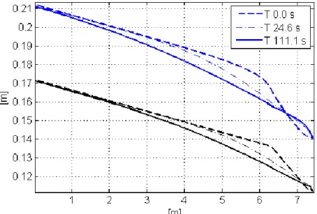
The evolution of an abrupt transition from a mild slope reach to an oversteepened reach downstream, for a steady discharge over mobile bed, has been modeled. The flow regime changes from subcritical to supercritical at the knickpoint, which is associated with a high sediment transport rate and erosion potential. This is a typical situation related to natural stream evolution phenomena.

The knickpoint progressively migrates upstream until the difference in slope between the two reaches tends to vanish. The cross section of the channel is rectangular, 0.5 m wide. The channel is 7.4 m long. The bed elevation at the upstream and downstream sections is fixed; the sediment diameter is set to 0.0016 m with density ρs = 2650 kg/m3 and bed porosity is 0.4.

The knickpoint is initially located at 6.3 m from upstream cross section. Discharge is 0.0098 m3/s

and no sediment feeding is provided. Downstream water level is kept at 0.14 m. Engelund-Hansen formula has been used:

𝑄

𝑠

= 0.05𝜌

𝑠

𝑔𝐵𝑈

2

√

_{𝑔(𝑠−1)}𝑑𝑠

(

_{𝜌𝑔(𝑠−1)}𝜏0

)

3/2

(2.32)

In Equation (2.32), Qs is the sediment discharge in volume, B is the channel width, ρ and ρs are the

densities of water and sediments, respectively; s is the relative density ρs/ρ; ds is the sediment

representative diameter; U is the water average velocity; τ0 is the bed shear stress.

The smoothing of the knickpoint is modeled correctly, as can be seen from free surface and bed profiles in Figure 7.

(28)

Figure 7. Free surface profiles and bed profiles variation for a knickpoint migration test.

(29)

Control of river bed degradation downstream an hydropower plant 17 |

Chapter 3 Control of river bed degradation downstream a run-of-the-river

hydropower plant

This chapter reports about an attempt to integrate the understanding of the river geomorphological dynamic into planning of optimal operation rules for a barrage serving a run-of-river hydropower plant (Bernardi et al., 2013; Dinh, 2014; Bizzi et al., 2015). Physically based one-dimensional hydrodynamic and sediment transport modeling, surrogate modeling techniques and Multi-Objective (MO) optimization are combined together in this framework, in a multidisciplinary approach.

The case study is a run-of-the-river power plant on the River Po (Italy) located in the Municipality of Monticelli d’Ongina (Piacenza), Isola Serafini. The objective is to assess if a better management policy of the barrage serving Isola Serafini exists, able to mitigate the river bed lowering processes occurring downstream the barrage without affecting significantly the hydropower production. A vast amount of literature has studied the effects of dams and barrages on river systems in terms of both geomorphological and ecological responses (Poff and Hart, 2002, Gurnell, 2005, Gupta et al., 2012.) Dams affect the hydrological regime downstream primarily through changes in timing, magnitude and frequency of high and low flows. Sediment connectivity is altered too, since a large amount of sediment load delivered by the headwaters upstream is trapped.

In response to the altered water and sediment fluxes, the river aims to a new equilibrium by a complex range of geomorphological adjustments which can undertake several steps and last many decades before reaching a more stable condition. Alterations include changes in cross-section (aspect ratio), bed material (e. g. coarsening), slope, pattern and bedforms. By trapping sediment

(30)

18 | Control of river bed degradation downstream an hydropower plant upstream, reservoirs can often cause the river transport capacity to exceed the available sediment supply, creating a sediment deficit downstream (Grant, 2003), which in turn triggers river erosion both on the river bed and the banks. Such adaptation processes can extend over hundreds of kilometers and last for decades.

Few frameworks have been developed to provide flexible decision making tools to assess the effects of building a dam in a specific catchment location (Grant 2003, Burke 2009). Nevertheless, when planning operating rules, only the fulfillment of the main purpose for which the structure is built is considered, very often hydropower production or water supply.

Multi-objective (MO) approaches can take into account a variety of water related interests affected by the dam construction, from flood mitigation to water supply and environmental quality and have been adopted to provide decision makers and stakeholders with valuable tools to measure the consequences of alternative operating rules from a variety of perspectives (Castelletti 2007, Yin 2009). These experiences have marked a significant progress in our ability to plan sustainable management of water resources and have provided more comprehensive insights of how dams affect the fluvial system and the related ecosystem services; however, the integration of fluvial geomorphological processes understanding when planning optimal operating rules remains very rare.

Studies that have optimized dam regulations in order to minimize their impact on channel morphological adjustments downstream are almost absent: we could find only one example in literature (Nicklow and Mays 2000, Nicklow and Ozkurt 2003). In this attempt, the authors built a single objective framework, i.e. the model is able to consider only the effect of operating rules on downstream river bed incision neglecting conflicts with other water related interests, like hydropower revenue or water supply as commonly addressed in a MO approach.

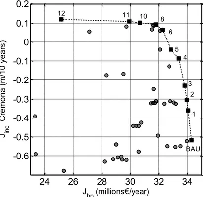
We then analyze the effects, in terms of hydropower revenue and river bed incision rate, of alternative operating rules over a time horizon of 10 years. To evaluate the effects of the different policies, a physically based one-dimensional numerical model has been used. A MO problem

(31)

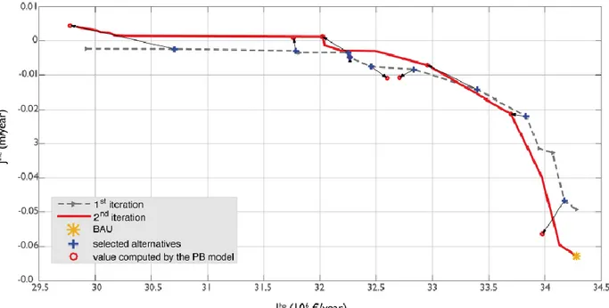
providing optimal solution, in a Pareto sense, for the two conflicting management objectives is then solved, by adopting a Response Surface approach. The following sections provide information on the modeling structure and present the results obtained.

The proposed case study aims to provide river managers with tools to critically compare the effects of alternative operational policies at the barrage in terms of river geomorphic processes. The findings allow analyzing the trade-off between hydropower production and river bed incision, and open the way to plan sustainable and cost-effective measures in the long term.

The work reported in this chapter has been carried out together with the group of Professor Rodolfo Soncini-Sessa at Politecnico di Milano University; Simone Bizzi, Quang Dinh and Simona Denaro.

3.1 Introduction to the case study: the Po river and Isola Serafini

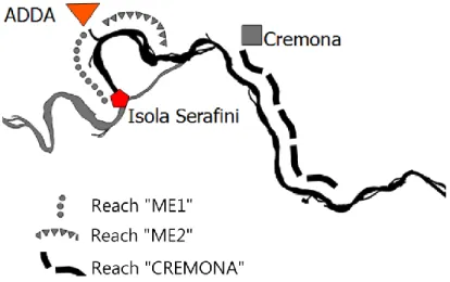
The Po is the longest river in Italy and runs for 652 km across the northern regions from the Alps to the Adriatic Sea, with a catchment area of approximately 70,000 km2. We have focused on a 112 km

long stretch in the river middle course (Figure 8) from Piacenza to Boretto, which includes the run-of-river plant of Isola Serafini.

Isola Serafini power station (Figure 9), managed by the Italian energy agency ENEL, is served by a 350 m wide barrage, located 16 km downstream Piacenza; it has a total capacity of 80 MW nowadays and has been operating since 1962. The incoming discharge is partially diverted to the hydropower plant channel on the right, which originated as a meander cut-off during the huge 1951 flood and joins again the Po river about 12 km downstream the gate, after a large meander.

(32)

20 | Control of river bed degradation downstream an hydropower plant

Figure 8. Location of the reach of interest.

The barrage has eleven sluice gates of equal width: In two of them, for sediment-scouring purposes, the bottom is lowered by 1.5 m. Six gates can be overtopped and work as sharp-crested weirs. There is no room for water storage behind the barrage, except for the short transitories during manoeuvres; thereafter, pondage is not a management option.

River Po environmental services are widely exploited. For instance River Po is the longest waterway in Italy and is the main irrigation supply to Po Valley, the richest and most productive agricultural area in Italy. Its high quality sands are suitable for constructions and were significantly exploited in the past decades.

Due to intense sediment mining as the main cause, the middle course of Po underwent a strong river bed degradation process in the years from 1950 to 2000 (Figure 10).

Sand mining was very intense from 1950 until 1980; after that, stricter regulations have first reduced and then stopped the activity. Surian (2003) state that instream mining increased from about 3 million m3_{/year to about 12 million m}3_{/year in the period 1960-1980, and then it}

decreased back to about 4 million m3_{/year. The peak volume (12 million m}3_{/year) is estimated to}

be not far from the assessed average annual sediment yield of the basin. Licensed amount in 1980 for instream mining was around 6 million m3_{/year (Italian Ministry of Agriculture, 1990):}

(33)

estimating a double amount is then realistic, controls from public authorities were insufficient at the time.

Figure 9. Aerial view of Isola Serafini run-of-river hydropower plant (flow upwards). The barrage diverts part of the flow to the power station on the right.

Along with sediment mining, also low water training for navigation purposes and the presence of dams in the upper part of the Po basin affect the overall sediment balance along the middle course. Besides, the presence of the IS hydropower plant plays an important role since its building in 1960. IS barrage is trapping sediment upstream, causing an abrupt decrease in sediment supply downstream and affects the hydrological regime reducing the transport capacity of the river in the meander downstream.

As a consequence of river bed lowering, several navigation and irrigation structures became unusable during low flow periods - e.g. harbor locks in Cremona, - forcing expensive interventions to rebuild them or restore their functionality. The estimated costs of the new dock in Cremona are over 40 million € (Bonomo, 2011).

(34)

22 | Control of river bed degradation downstream an hydropower plant For all these reasons, Isola Serafini run-of-river power station is a suitable case study where to assess the existence of an optimal operating rule balancing the conflicting needs of maximizing hydropower revenue and minimizing river bed incision rate downstream of the plant.

Figure 10. Minimum water levels recorded at Cremona gauging station.

3.2 Modeling the system: the power station operating rule

The current operating rule of Isola Serafini barrage is reported in Figure 12 (bold red line) and aims at maximizing hydropower production. For this purpose, the water level upstream the dam is constantly kept at 41.00 m a.s.l., with a maximum tolerance of 0.50 m. The power production is always maximized except during floods, when the power station is stopped for safety reasons. As previously recalled, no water pondage is allowed so continuity at the bifurcation is satisfied at any time.

Variable a is the inflow from upstream and u is the amount of water diverted to the hydropower plant, the decision variable; consequently w = a-u is the discharge downstream of IS (Figure 11). A MEF (minimum environmental flow) of 100 m3_{/s is required through the meander at any time and}

the minimum flow to activate a turbine of the power station is 200 m3_{/s; so, for incoming}

1950 1960 1970 1980 1990 2000 27.5 28 28.5 29 29.5 30 30.5 31 31.5 32 years

M

inim

um

w

at

er

lev

el

(m

)

(35)

discharges a not greater than 300 m3_{/s, the power station is not working and the diverted flow u is}

null.

When a is greater than 300 m3/s, all flow exceeding MEF is diverted to the turbines, until the

maximum permitted of 1000 m3/s, so as to maximize electricity production. For a = 1100 m3/s or

greater, then, the power station keeps working at his maximum capacity; all incoming flow exceeding this value passes throughout the gate and flows into the meander.

The station can work until the total incoming discharge reaches approximately 4000 m3_{/s; above}

this threshold, the head jump across the gate becomes too low for electricity generation so all the turbines are switched off (u = 0). In addition, to avoid flooding risk, all gates must be completely open to let the flood pass through.

Figure 11. Scheme of the case study.

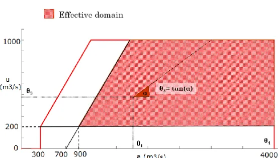
In order to build alternative regulation policies, we parameterized the current operation rule. The physical constraints for the variables are given by the MEF in the meander, the minimum and maximum flow through the turbines and the safety limit against flood risk. In addition, to enclose

(36)

24 | Control of river bed degradation downstream an hydropower plant the alternatives in an effective domain, a critical value of the discharge Qcrit must be defined, i.e. a

value of discharge below which sediment transport can be considered negligible. Recent modeling studies in Po river (Rosatti, 2008) stated Qcrit equals 800 m3/s. This threshold has been decreased to

700 m3/s.

Figure 12. Current Isola Serafini operating rule and domain of alternatives.

Alternative policies should be planned to reach two main purposes: the increase of the sediment supply to the downstream reach and the increase of the transport capacity in the meander to mobilize settled sediment. Moreover, they should conflict as less as possible with the hydroelectricity production.

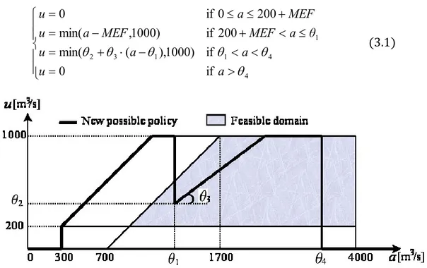
The operation rule can be defined by a class of piecewise-linear functions (such as the BAU operating rule or a new one e.g. bold black line in Figure 13), specified by a vector containing a set of 4 elements, θ1, θ2, θ3 and θ4. The fourth parameter, θ4, is the discharge threshold at which the

gates are completely open. This parameter affects primarily sediment supply to the downstream reach and secondly also the transport capacity in the meander; θ1, θ2, and θ3 affect mainly transport

capacity in the meander by reducing the discharge u through the turbines (so increasing the discharge through the barrage) when the power station is on. In detail, θ1 and θ2 are the

(37)

coordinates of a point in the effective domain and θ3 is the slope of the line connecting (θ1,θ2) with

the boundary of the domain (see Figure 13) The class of functions is defined as follows:









































4 4 1 1 3 2 1

if

0 if

)

1000

),

(

min(

200 if

)

1000

,

min(

200

0 if

0 



a

u

a

u

θ

a

MEF

a

u

MEF

a

u

(3.1)

Figure 13. Domain of alternatives with a new possible policy diagram

Taking care of all constraints, the feasible effective domain is specified by the following conditions:

















1

0 )

1000

,

700 min(

200

900 4000

2000

3 1 2 4 1 4



(3.2)

The business as usual operating rule (Figure 12), for instance, can be obtained by setting θ1 ≥ 300;

(38)

3.3 Modeling the physical system: hydrodynamics and sediment

transport

Before describing the model building steps, it is worth recalling that the results of hydro-morphological modeling are more significant in terms of comparison between different operating rules rather than looking at absolute values. The inherent uncertainty in modelling morphological processes also suggests this precaution.

To represent correctly the river bed evolution processes at the reach scale over a 10-years horizon, and to avoid overburdening computational times, given the high number of simulations to run, the choice fell on a one-dimensional hydro-morphological model able to represent 1D flows with mobile bed in natural channels of complex geometry. We elaborated the model presented by Schippa and Pavan (2009) and adapted it to the specific requirements of the case study.

The main features of the mathematical model can be found in Chapter 2. The model is based on a set of three differential equations (equations (2.1)-(2.3) in Section 2.1) stating mass and momentum conservation for the liquid phase (shallow water equations) and mass conservation of the solid phase (Exner equation) along the main stream direction. We recall them here:

𝜕𝐴 𝜕𝑡

+

𝜕𝑄 𝜕𝑥

= 𝑞

(3.3)

𝜕𝑄 𝜕𝑡

+

𝜕 𝜕𝑥

(

𝑄2 𝐴

+ 𝑔𝐼

1

) = 𝑔

𝜕𝐼₁ 𝜕𝑥

|

− 𝑔𝐴𝑆

𝑓

(3.4)

(1 − 𝑝)

𝜕𝐴𝑏 𝜕𝑡

+

𝜕𝑄𝑠 𝜕𝑥

= 𝑞

𝑠

(3.5)

The finite difference explicit scheme developed by McCormack (1969, see section 2.2) has been chosen to integrate the system of governing equations.

As stated in Chapter 2, two closure equations are needed to solve the system, for friction slope Sf

and sediment discharge Qs.

(39)

Control of river bed degradation downstream an hydropower plant 27 | 3 / 4 2 2 2

R

A

Q

n

Sf 

(3.6)

Where n is the Manning resistance coefficient, A is the cross-section wetted area, Q is liquid discharge, R is hydraulic radius.

For sediment discharge, the Engelund-Hansen (Equation 3.7, Engelund and Hansen, 1964) formula has been chosen. Previous studies on the Po river (Italian Ministry of Agriculture, 1990) have shown that this formula, compared to others, is the most suitable to correctly represent sediment movement in the Po river. Since then, no more complete field campaigns about sediment transport all along the Po have been performed.

Moreover, Engelund – Hansen formula has several advantages: it is simple to implement, and it is a total transport formula. Being the grain size in the studied stretch (around 0.5 mm) well inside the applicability limits, we assessed that Engelund-Hansen formula could be a fairly accurate starting point. Of course, implementing a different formula for sediment transport in the model is straightforward. 2 / 3 0 2

)

1 (

)

1 (

05 .

0 _





















s

g

s

g

d

gU

q

s s s

_





(3.7)

In (3.7), qs is the solid discharge per unit width; ρ and ρs are the densities of water and sediments,

respectively; s is the relative density ρs/ρ; ds is the sediments representative diameter; U is the

water average velocity; τ0 is the bed shear stress.

Engelund-Hansen formula is used also to calculate sediment contribution from the tributaries. Cross section features of the tributaries at the mouth and data about the slope and sediment diameters are reported in Po Acquagricolturambiente (Italian Ministry of Agriculture, 1990).

(40)

28 | Control of river bed degradation downstream an hydropower plant The cross sections along Po river are available from the topographical surveys by AIPO (Interregional Po Agency), carried on in 2009. There are 67 surveyed cross sections in the reach of interest, one every 1.69 km in average. On every cross section plot, the boundaries of the overbanks and the thalweg are identified: then, to improve spatial accuracy, cross sections are linearly interpolated up to a distance of 450 m, i.e. the number of cross sections along the reach is increased to 250. Flow resistance coefficients were calibrated during previous studies (Schippa et al., 2006)

Figure 14. Cross section plot.

The river stretch is split in two sub-stretches, A from Piacenza to IS gate and B from IS to Boretto (Figure 11). The first is 30 km long whereas the length of the second is almost 82 km. All 4 tributaries (Adda, Taro, Parma and Enza) join the river in reach B. The power station channel joins the river between the Adda confluence and Cremona.

At upstream boundary (Piacenza station) and along the lower course of the tributaries, a long time series of data is available from ARPA (Regional Agencies for Environment) records. We refer to a 10-year long historical time series of water inflows recorded at Piacenza and at the tributaries' mouths from 1964 to 1973. For this period, data are readily available and can be representative also for the future, since no relevant changes in the hydrological regime have occurred at basin scale.

(41)

At downstream station (Boretto), the stage-discharge relationship is provided by ARPA hydrological bulletins as well.

A specific subroutine implements the control rule of the barrage, and makes the model switch between two different operating conditions.

Case 1. When the power station is on, (a <= θ4, see section 3.2), the water level upstream the

barrage is kept at 41 m a.s.l. and the two reaches A and B are disconnected. This means that the upstream boundary condition for reach A is the inflow at Piacenza, whereas the downstream boundary condition is the imposed water level.

The operating rule of the barrage provides the upstream boundary conditions for reach B , namely water and sediment discharge entering the meander. Downstream condition for reach B is provided by the stage-discharge relationship.

It is evident that we do not include in the model the numerical solution for the equations in proximity of the barrage: this purpose is clearly beyond the scope of our work, for the complexity of the physical phenomena occurring when the flow approaches the gates. The equations we use for the 1D model are no longer valid in the area close to the gates, clearly dominated by 3D flow patterns.

For these reasons, modeling the sediment transport across the barrage, taking into account all the local physical processes, requires assumptions to introduce a simplification keeping as close as possible to reality. In Case 1, when the power station is operating and the gates are at least partially closed, Qup,B -the sediment discharge entering stretch B, is calculated as

7 . 1 , , 0.7          a w Q Q_up_B _dw_A

(3.8)

Where Qdw,A is the sediment discharge approaching the barrage, w is the liquid discharge flowing

(42)

30 | Control of river bed degradation downstream an hydropower plant The empirical reduction coefficient - 0.7 - is applied to take into account the fact that not all of the eleven gates are open when power station is operating, so part of the sediment is retained. Anyway, it has to be noticed that when power station is on, water velocity and transport capacity close to the barrage are really small: the backwater effect slows down the flow well before getting to the barrage, so the sediment supply to the downstream reach is limited.

Case 2. When the flow rate is above the safety limit against flood risk (a > θ4, see section 3.2) all the

gates are fully open. No flow is diverted to the power plant channel (u = 0, see Figure 11) and the two reaches A and B are linked, without an internal boundary condition.

In Po Acquagricolturambiente (Italian Ministry of Agriculture, 1990), it is stated that most of the sediments taking part in the bed evolution processes are transported, during high flows, in suspension and only a small part by traction near the bed; so we decided, as a first step, to assume that for the highest flows, with all gates of the barrage open, nearly all sediments pass through the gate. Moreover, the opening of the gate and the subsequent increase in flow velocity in the adjacent zone upstream, if compared to the condition of barrage closed, could bring back in suspension previously settled fine material and convey it downstream. A study by the Po River basin management authority (AdbPo, 2007) shows that material with diameter up to 1 ψ (0.5 mm) can be transported in suspension. For this reason we decided to assume that full continuity is satisfied also for sediment transport.

(43)

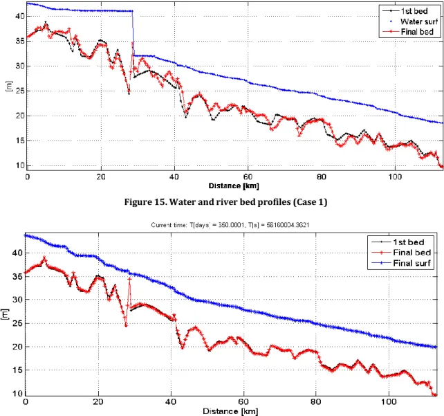
Figure 15. Water and river bed profiles (Case 1)

Figure 16. Water and river bed profiles (Case 2)

3.4 Indicators

The two conflicting objectives of hydropower production revenue and reduction of river bed incision are quantified through suitable indicators, in order to implement them in the optimization process.

The physically based model simulation provides a final configuration of the bed (e.g. Figure 15). A low-discharge, steady flow simulation (300 m3/s) is run over both the initial and final bed

configurations. The two water surface profiles are then compared and an indicator of river bed incision is calculated measuring the difference in water levels, zwfinal - zwinitial.

(44)

32 | Control of river bed degradation downstream an hydropower plant To obtain the first indicator Jinc for a specific sub-reach, water level variations are averaged over the

M cross sections belonging to it.

M j initial final inc

avg

zw

J

.... 1

)

(







(3.9)

The indicator Jinc can be calculated for specific sub-reaches all along the river stretch, to investigate

the system behavior.

This indicator is quite reliable: water level for a low-discharge event is able to smooth and compensate local effects, if compared to indicators referring to river bed level alone. It has a drawback though: it cannot be computed during the observation period, but only as a difference between final and initial state because an additional steady flow simulation is needed. This makes it suitable for a feed-forward approach, where outcomes of a selected alternative are checked at the end of the simulation period.

In preparation for a feedback/feedforward framework (see Section 3.7) in which real-time monitoring of river bed incision is planned, another indicator has been chosen. We monitor the evolution of the bed level in 5 pre-specified points within the main channel bed (one is the thalweg, the other four are two on its left and two on its right side) in each one of M cross sections equally distributed along the reach of interest.

Figure 17. Indicator for river bed incision: 5 points monitoring. Example

3800 3900 4000 4100 4200 4300 4400 4500 4600 0 0.5 1 1.5 2 2.5 3 3.5 4 4.5 XS 30, Distance (km) = 9.56 XS Left thw,1 Left thw, 2 Thalweg Right thw, 1 Right thw, 2

(45)

Let's denote with zb,ij (0) the bed level in the i-th point (i=1, …, 5) of the j-th cross section (j=1,…,M)

the first day of the y-th year of the evaluation horizon. The bed level variation Jy in the reach

downstream from Cremona at the beginning of the y-th year is then defined as the average difference of level between time zero (the starting of the evaluation horizon) and that instant all over the sampled points, i.e.

 

 





5 ... 1 1... , ,

(

)

(

0 ))

(

5

1

i j M ij b ij b y

z

y

z

M

J

(3.10)

The indicator of total river bed incision can be considered as Jy for y = N, where N is the number of

years in the evaluation horizon. It is convenient, however, to refer to an average incision rate per year

N

J

N

inc



(3.11)

If J is negative – in both versions (3.9) and (3.10) - we may assume that the river bed is undergoing degradation. It is evident that it is not possible to condensate all information related to river morphological evolution in a single indicator without strong simplifications: however, Jinc is

certainly representative of an overall erosion (or deposition) trend occurring in the analyzed river reach.

As for hydropower , the revenue of hydropower (€) over n days is the sum of the product of the daily energy production Pt (kWh) by a time-varying energy unit price πt. This revenue can be

divided for the number of years N to obtain a yearly revenue (€/year):









n t t t hp

P

N

J

1

1 _

(3.12)

In turn, the daily production Pt is given by the product of water density ρ and gravity acceleration g

by the flow release u through the turbines, the head jump H and the turbine efficiency η (with . H is the difference between the water level upstream the gate and the level just downstream the turbines (hup - hdown).

(46)

t

H

u

g

P

_t







_t _t _t

(3.13)

In turn, the daily production Pt is given by the product of water density ρ and gravity acceleration g by the flow release u through the turbines, the head jump H and the turbine efficiency η and the time. H is the difference between the water level upstream the gate and the level just downstream the turbines (hup - hdown). Since flow profile in the power station channel is not calculated, hdown is

given by an empirical relationship: hdown = f(u, hjunc). The dependent variables are the discharge u

flowing into the channel and the water level at the junction between the channel and the Po river (hjunc, computed by the model).

3.5 Problem formulation and design of experiments

We already defined (section 3.2, Figure 11): a (incoming flow), u (flow diverted to the HP station) and w (residual flow passing through the gates). The flow u is led back into the main channel a few km downstream. The multi-objective design problem, following the formulation of Soncini-Sessa et al., (2007) for water resources problem, can be so formulated:

𝑚𝑖𝑛|

_𝜃

J (𝒙

_{𝑡=0→ℎ−1,}

𝑢

_{𝑡=0→ℎ−1,}

𝑎

_1→ℎ

)

𝑥

_𝑡

= 𝑓 (𝒙

_𝑡−1

, 𝑢

_𝑡−1,

𝑎

_t

)

𝑢

𝑡

= m(𝑎

t

, 𝜽)

t = 0,1, … , h

(3.14)

a is the incoming flow from time 1 to time h (given). The management objectives pursued (see sect. 3.4, hydropower production revenue and reduction of river bed incision) are expressed by the indicators Jhp and Jinc that condense the information provided by the hydromorphological model f.

We seek optimal operating rules m (function of the inflow a and the design parameter vector θ with the four parameters θ1,… , θ4 listed in sect. 3.2) to maximize both Jhp and Jinc . The physically based

model f gives us information on the states x (water and river bed levels) at time t provided we have information on states at time t-1 and we chose an operating rule m among the feasible rules.

ONE-DIMENSIONAL HYDRODYNAMIC MODELS IN RIVER RESOURCE MANAGEMENT AND POLICY DESIGN

Università degli Studi di Ferrara

DOTTORATO DI RICERCA IN

SCIENZE DELL’INGEGNERIA

CICLO XXVII