U
NIVERSITÀ DI
P
ISA
DIPARTIMENTO DI INGEGNERIA CIVILE E INDUSTRIALE
TESI DI LAUREA MAGISTRALE
INGEGNERIA AEROSPAZIALE
Multi-physic simulation for an All Electric Aircraft on board systems
for the assessment of electrical power absorptions
Relatori:
Prof. Eugenio Denti Ing. Francesco Schettini
Candidato:
Alessandro Argemandy Naghad
Abstract
This thesis gives a contribution to the fulfilment of a numerical tool named Shared Simulation Environment (SSE) developed at the University of Pisa within the Clean Sky GRA AEA European project. This tool aims at the dynamic simulation of the electrical energy absorption of the various on-board systems during the manoeuvres of the new all-electric Green Regional Aircraft (GRA).
In the GRA an appropriate management of the electrical power available aboard is required to avoid generator overloads or temporary lack of energy for powering safety-critical systems. The SSE is developed in order to permit the design and the validation of the electrical Energy Management Logics under development within the project. The thesis describes the methodologies used to develop a prototype of the SSE by integrating models coming from different simulation environments (Simulink, AMESim, Dymola). It also depicts the architecture of the prototype itself and describes the effects on the computation time of different integration methods, together with some preliminary simulation results.
Index
List of figures……….6
List of tables………..8
Acronyms………..9
Introduction…………..….………..10
1 Shared Simulation Environment ... 13
2 Mission Profile ... 16
3 Electrical Power Generation System ... 19
3.1 Machine description ... 21 3.1.1 Main alternator ... 21 3.1.2 Excitation stage ... 21 3.1.3 Rotating diodes ... 21 3.1.4 PMG ... 22 3.1.5 Cooling ... 22 3.2 Simulink Model ... 22 3.2.1 Generator ... 22 3.2.2 GCU ... 23 3.2.3 Load ... 25
4 Environmental Control System ... 27
4.1 Model inputs ... 27
4.2 Model outputs ... 28
5.1.2 Parameters and interfaces ... 34
5.2 AMESim – Simulink Interface ... 35
5.2.1 Preliminaries... 36
5.2.2 Interface block ... 36
5.3 Encryption of an AMESim model ... 39
5.4 Linear Analysis of the model ... 42
6 Simulation Analysis ... 46
6.1 Simulink Environment ... 46
6.1.1 “Stand alone” mode ... 46
6.1.2 Co-Simulation mode ... 49
6.2 Simulation Parameters in Simulink ... 51
6.3 Simulation Parameters in AMESim ... 54
7 Cabin Thermal Model: Closed Loop Analysis ... 56
7.1 Temperature controller ... 56
7.2 Pressure controller ... 58
7.2.1 Pressure controller with butterfly valve ... 60
8 Energy Management System ... 62
8.1 EMS Supervisory Control Strategy ... 62
8.2 Dymola – Simulink Interface ... 63
9 Simulation Run and Results ... 65
9.1 Initial trim procedure ... 65
9.2 “Dummy” input data ... 66
9.3 “Flight history” input data ... 72
Conclusions………. 84
List of figures
Figure 1.1 SSE prototipe ... 13
Figure 2.1 From Workspace block ... 16
Figure 3.1 CGU – Generator interface ... 19
Figure 3.2 Three-stage brushless synchronous machine description ... 20
Figure 3.3 Limits for DC over-voltage and under-voltage for 270 VDC system ... 25
Figure 4.1 Standard quantities ... 29
Figure 5.1 Thermal Architecture Model ... 32
Figure 5.2 Solar radiation intensity vs. aircraft altitude (MIL-E-38453A) ... 33
Figure 5.3 AMESim – Simulink Interface ... 36
Figure 5.4 Interface Icon Creation dialog box ... 37
Figure 5.5 AMESim Interface Block ... 38
Figure 5.6 S-Function dialog box ... 38
Figure 5.7 Simulink S-Function block associated to the AMESim model ... 39
Figure 5.8 Supercomponent in AMESim ... 40
Figure 5.9 Supercomponent dialog box ... 41
Figure 5.10 Encryption of a Supercomponent ... 41
Figure 5.11 Time step response ( ) ... 44
Figure 5.12 Bode diagram ( ) ... 45
Figure 6.1 AMESim – Simulink interfaces ... 49
Figure 6.2 Interface Icon Creation dialog box ... 50
Figure 6.3 Co-Simulation mode Parameters ... 50
Figure 6.4 SSE – preliminary tests ... 53
Figure 6.5 Absolute and Relative tolerance ... 54
Figure 6.6 AMESim simulation parameters ... 55
Figure 7.1 Retroaction scheme ... 56
Figure 9.4 “Dummy” results – Control Surfaces Deflection ... 68
Figure 9.5 “Dummy” results – Flap Deflection ... 68
Figure 9.6 “Dummy” results – LG Extraction/Retraction ... 69
Figure 9.7 “Dummy” results – EPGS Voltage and Current ... 69
Figure 9.8 “Dummy” results – ECS Outlet Temperature and Mass flow ... 70
Figure 9.9 “Dummy” results – CT Temperature & Pressure ... 70
Figure 9.10 CT Temperature (zoom) ... 71
Figure 9.11 “Dummy” results – Electrical Power and Currents Absorbed ... 71
Figure 9.12 “Dummy” results – Electrical Power and Currents Absorbed (zoom) ... 72
Figure 9.13 Flight history input data – Mach, Altitude ... 73
Figure 9.14 Flight history input data – Aerodynamic Angles ... 73
Figure 9.15 Flight history input data – Linear Accelerations ... 74
Figure 9.16 Flight history input data – Euler Angles ... 74
Figure 9.17 Flight history input data – Angular Velocities ... 75
Figure 9.18 Flight history input data – Angular Accelerations ... 75
Figure 9.19 Flight history input data – Engine ... 76
Figure 9.20 Flight history input data – ECS commands ... 76
Figure 9.21 Flight history input data – Control Surfaces Deflection ... 77
Figure 9.22 Flight history results - Control Surfaces Deflection ... 78
Figure 9.23 Flight history results – Flap Deflection ... 78
Figure 9.24 Flight history results – LG Extraction/Retraction ... 79
Figure 9.25 Flight history results – EPGS Voltage and Current ... 79
Figure 9.26 Flight history results – ECS Outlet Temperature and Mass flow ... 80
Figure 9.27 Flight history results – CT Temperature & Pressure ... 81
Figure 9.28 Flight history results - Pressure target ... 81
Figure 9.29 Flight history results – CT Temperature (zoom) ... 82
Figure 9.30 Flight history results – Electrical Power and Currents Absorbed ... 82 Figure 9.31 Flight history results – Electrical Power and Currents Absorbed (zoom) . 83
List of tables
Table 3.1 Generator performances ... 19
Table 3.2 Generator parameters ... 23
Table 3.3 Generator Inputs/Outputs ... 23
Table 3.4 GCU Inputs/Outputs ... 24
Table 3.5 Load Inputs/Outputs ... 25
Table 4.1 ECS model characteristics ... 27
Table 4.2 Turbomachines parameters ... 30
Table 4.3 Heat Exchanger parameters ... 30
Table 4.4 Valves parameters ... 30
Table 4.5 Sensors parameters ... 30
Table 5.1 Thermal Architecture Model external interfaces ... 35
Table 6.1 Preliminary tests - Computational times ... 48
Acronyms
A/C Aircraft
CT Cabin Thermal
ECS Environmental Control System
EMS Energy Management System
FCS Flight Control System
GRA Green Regional Aircraft
LGS Landing Gear System
SSE Shared Simulation Environment
Introduction
This work is performed within the Clean Sky European project – Green Regional
Aircraft (GRA) platform – All Electric Aircraft (AEA) domain. The goal of Clean Sky
is to achieve significant improvements in the environmental impact of aviation. In this direction, the recent trend aims at the electrification of all aircraft systems, even if challenging issues about the management of the on-board power arise in this approach. The AEA concept is based on the removal of the sources of pneumatic power (from the engine) and hydraulic power, and replace them with the electrical one. This objective can be only achieved by properly monitoring and managing the power requests (e.g. by temporarily reducing the power supplied to some systems during those flight phases in which the total request of electrical power could overcome the maximum available). In this work, a first contribution to the fulfillment of a numerical tool, able to support the design of the electrical power generation and distribution system, will be illustrated. This particular tool is a simulation software, named Shared Simulation Environment (SSE) that can support the design and the validation of the electrical energy management strategies to be implemented aboard an all-electric GRA. The SSE integrates simulation models realized according to the All-Electric concept and able to reproduce the functions and the main performances of on-board systems, with particular attention to the power absorption issues. These models are developed by dividing the work among the Clean Sky partners (Alenia Aermacchi, EADS CASA, Liebherr-Aerospace Toulouse SAS, Thales A.E.S. – France, Airgreen cluster), according to three levels of increasing complexity: Architectural, Functional and Behavioural:
Level 1: Architectural level - Simple, non-dynamic models for the preliminary energy consumption assessment
Level 2: Functional level - Combination of steady-state and simple dynamic models for the preliminary analysis of energy management strategies, in the
are in general not suitable to be integrated in the SSE context. This is because, by disregarding the dynamic dependencies between inputs and outputs, the architectural level models lead to algebraic loops in the whole system. The solution of these algebraic loops can be difficult and can lead to models of a poor physical meaning. For this reason, architectural level models are not integrated into the SSE, except for some systems that, from the point of view of energy absorption, are to be modeled in a very simple way, as pure resistive loads.
As for the behavioural level models, the first experience about SSE integration showed that the computation time is the most important issue for the SSE and the use of behavioural level models, which are the most time-consuming ones, should be limited to the cases of real need. So, not all models will be integrated at level 3. In addition, the level 3 models will be always accompanied by the corresponding level 2 ones, to give the SSE user the possibility of choosing between models of level 2 (for simulations of longer A/C manoeuvres) and level 3 (for shorter simulations, carried out to investigate some phenomena in more detail). This will improve the efficacy of SSE.
These models are developed using three different software: - AMESim (ver11.2.0 / Rev11 SL2)
- Dymola (ver2013)
- MATLAB/Simulink (verR011b/7.8)
The first two are Object Oriented Software, differently by the last one, i.e. they give the user the possibility to access to a set of libraries (mechanical, electrical, pneumatic, hydraulic, etc...) and to find a set of already built components (but even to create new ones), where one can modify all the parameters useful for a simulation. The great benefit is to create a system just assembling the elements it is composed by, and, on the other side, to simulate the dynamic behaviour among various systems, which belong to different physic domain. In Simulink, instead, the user has to develop all the equations of each system, which often are not linear differential equations.
MATLAB/Simulink was chosen as main simulation environment because the major part of the models was developed using this software, the synthesis of the control laws is easier, it has not given particular problem during the simulation tests.
The thesis studies the methodologies that can be used to connect and run models coming from different simulation environments (Simulink, AMESim, Dymola), thus building a common integrated environment.
In the first part of this document all the models involved in the construction of the SSE are analysed (chapter 1-6), in details: the input data for the simulation, the Electrical Power Generation System (EPGS), the Environmental Control System (ECS), the Cabin Thermal (CT) model, with particular attention to the AMESim environment and its interface with Simulink, the closed loop between the CT and the ECS (chapter 7). At this point the first tests, the methodologies of simulation, the choice of the Simulink solver and integration step are described. In chapter 8 then, we can find the Energy Management System (EMS), the last block for the SSE and the implemented strategy to optimize the electric power distribution. Moreover the attention is put on the interface between Dymola and Simulink. Finally, in chapter 9, there are presented two different simulation tests with their results, and the procedure to “trim” the entire model because the SSE is designed to simulate a flight mission starting from steady flying conditions. This goal was been achieved via dynamic simulation.
1 Shared Simulation Environment
The SSE is, de facto, a scheme that includes the models of the most important on board aircraft systems. It is developed in Simulink and contains the interfaces with AMESim and Dymola to exchange data throughout a simulation run.
It is composed by several blocks: - Mission Profile
- Engine
- Electrical Power Generation System - Energy Management System
- Flight Control System - Landing Gear System - Ice Protection System
- Environmental Control System - Other Systems
- Global Thermal A/C Architecture - Temperature Controller
- Pressure Controller - Simulation time - Output Storage
The first block provides the input simulation data and will be detailed described in the next chapter. The second one contains information about the aircraft engine where the only information is the engine RPM.
The third one contains the electric generator dynamic model and it is directly connect to the EMS.
The FCS block describes the dynamic behavior and the deflection of all control surfaces (ailerons, rudder, elevators, inboard and outboard flaps, inboard and outboard spoilers). It is developed in a previous thesis of University of Pisa, ref[1].
The LGS block describes the extraction and retraction of landing gear system and it is developed in a previous thesis of University of Pisa, ref[2].
The last two blocks are only useful for the simulation run, the first one to see the time and to decide when enable a single system, the second one to organize each variable to plot.
2 Mission Profile
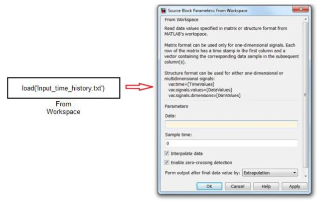
As said in the previous chapter, this “subsystem”, so called in the MATLAB/Simulink ambient, provides the data input for a generic simulation run.
From the Simulink library, in particular in the Sources section, one can select the block
From Workspace which gives the user the possibility to load data in a matrix form and
then split them into different signals with a Demux block.
It is very important that the first column of the matrix data is dedicated to the time, so the software can evaluate each variable at each moment. Between two generic integration steps, a linear interpolation is performed.
values (Input_time_history.txt) and the second one the explanation and the measurement unit of each variable (Input_time_history_explain.txt).
Once the data are loaded and split, they are organized into three different sections: - Environmental Conditions
- A/C Flight Data - Pilot Commands The first section contains:
- Altitude, “h”
- Air Density, “rho” - Air Temperature, “T” - Air Pressure, “P” - Mach number,
All the atmospheric conditions are calculated using an ISA Model implemented into a Simulink block, which is located in the Aerospace Blockset section.
The second section contains the flight data related to the aircraft: - Speed, “Speed”
- Angle of attack, “alpha” - Angle of sideslip, “beta” - Load factor x, “nx”
- Load factor y, “ny” - Load factor z, “nz” - Roll rate p, “p” - Pitch rate q, “q” - Yaw rate r, “r” - Roll acceleration, ̇ - Pitch acceleration, ̇ - Yaw acceleration, ̇ - Roll angle, “phi” - Pitch angle, “theta” - Yaw angle, “psi”
Finally the last section includes the various commands: - Ailerons command, “da”
- Rudder command, “dr” - Elevators command, “de” - Flaps command, “df” - Spoilers command, “dsp” - Landing gear command, “dlg” - Throttle command, “thrust” - ECS activation,
- Cabin Reference Temperature, - ECS Power Increase,
- ECS Power Management order deny, - Thrust,
3 Electrical Power Generation System
The purpose of this machine, developed in Simulink by Thales, is to supply the electrical network of the aircraft; it composed by a generator driven by the engine, a CGU (Generator Control Unit) that regulates the voltage delivered by the generator itself and a rectifier diode, according to the following figure:
Figure 3.1 CGU – Generator interface Generator‟s performances are summarized in the following table:
Normal speed range
Output three-phase AC current
Output three-phase AC voltage
Efficiency
Output rectified DC voltage
Permanent output power
Table 3.1 Generator performances
Moreover the alternator weight does not exceed 25 kg with its internal oil and the V-band; excluding the V-band itself the weight of dry and empty alternator is 23.8 kg. The generator is a three stage brushless synchronous machine composed of:
excitation stage
permanent magnet generator (PMG)
The three elementary alternators are connected in cascade. The output of the PMG, supplies the excitation to the excitatory element, via the generator control unit (GCU). The output of the excitatory element is connected to the input of a rotating rectifier bridge. The DC current delivered by the rectifier bridge energizes the rotor of the main generator.
Figure 3.2 Three-stage brushless synchronous machine description
Machine description 3.1
3.1.1 Main alternator
The main alternator delivers the power to the electrical network via the feeders and the converter. Rotor (inductor)
Four salient poles
Dampers composed of copper bars soldered to a copper ring at each side of the rotor
Stator (armature)
Star-connected three-phase winding
Low loss Iron Silicon alloy laminations
Electrical insulation in 240°C class material
3.1.2 Excitation stage
The excitation stage has the following characteristics: the exciter inductor is supplied with a DC voltage in generating mode. Induced AC voltages are rectified by a rotating diode bridge.
Rotor (armature)
Star-connected three phase winding
240°C class varnish impregnation Stator (inductor)
Height salient poles
Laminations to reduce core losses in starting mode
3.1.3 Rotating diodes
The rotating six-diode three-phase bridge rectifies the AC voltages provided by the excitation stage.
1200 V, 60 A
Temperature working range: -55°C to 175°C
3.1.4 PMG
The PMG delivers power to the generator control unit (GCU), which controls generator output voltages, monitors and protects the generation channel. It is not modeled at this level.
3.1.5 Cooling
The generator is cooled by an oil spray (minimum oil flow: 10 l/min)
Simulink Model 3.2
It composed by three blocks: 1 Generator block model 2 GCU block model 3 Load block model
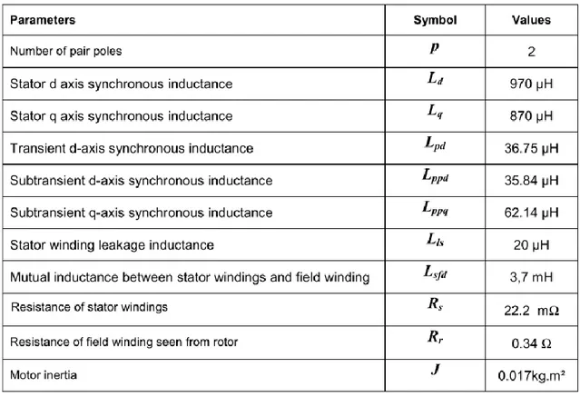
3.2.1 Generator
The first one is composed of the main alternator with saturation, a RC filter and a rectifier. The RC filter is placed at the output of the diode rectifier in order to smooth the DC output voltage. The values used for the simulation are 100 µF for the capacitor in series with a resistor of 0.5 Ω and 270 Ω for the resistor in parallel.
Table 3.2 Generator parameters
The following tables gives instead, the name and the type for the various ports that are used by the generator block.
Table 3.3 Generator Inputs/Outputs
3.2.2 GCU
Control loop of the output voltage
Protections
The following tables gives the name and the type for the various ports that are used by the GCU block.
Table 3.4 GCU Inputs/Outputs
The GCU protections included in the model are:
Over-current
Permanent load current: 259A at 12000rpm
5 min load current: 280A at 12000rpm
30s load current: 315A at 12000rpm
5s load current: 370A at 12000rpm
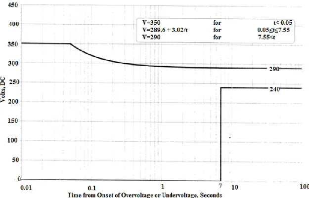
Under-voltage and Over-voltage
Figure 3.3 Limits for DC over-voltage and under-voltage for 270 VDC system
3.2.3 Load
The following tables gives the name and the type for the various ports that are used by the load block.
Table 3.5 Load Inputs/Outputs
It is important to underline, about the simulation run, that the user can modify only the following parameters:
Speed rpm: Value set by default at 12000rpm (the speed range is between 12000 and 20000rpm)
Resistive load: which is integrated into the LOAD block and which can be modified by another type of load
Threshold1, 2 and 3, which specify the limits of the current
4 Environmental Control System
In this chapter we will give few details about the ECS model, which is encrypted and was developed in Simulink by Liebherr-Aerospace. It simulates the dynamic behavior in closed loop conditions together with the control laws and the cabin model. It includes the transient modeling of ECS components through estimated transfer functions to describe the main dynamic effects (actuators behavior, component inertia, sensor time responses). Moreover the model include a simplified modeling of ECS static performances. The table below provides the main characteristics of the model:
Table 4.1 ECS model characteristics
Model inputs 4.1
Ambient conditions:
- Mach number - Altitude [ ] - OAT [ ]
A/C conditions (flight phases)
Ram-Air interface conditions:
- RAM Inlet Recovery Pressure [ ] - RAM Inlet Recovery Temperature [ ] - RAM Outlet Recovery Pressure [ ] - RAM Outlet Recovery Temperature [ ]
Electrical Power Available [ ]
Cabin environment data:
- current cabin temperature [ ] - current cabin pressure [ ]
ECS system targets (for A/C System Controls Coupling)
- Set-point for ECS Mass Flow provided to Cabin Control System [ ]
- Set-point for ECS Temperature provided to Cabin Control System [ ]
Model outputs 4.2
The ECS model provides the SSE with the following set of information and data:
ECS cooling performances (for A/C System Environment Coupling)
- Actual Mass Flow provided to Cabin Control System [ ] - Actual Temperature provided to Cabin Control System [ ]
Data list 4.4
This section is dedicated to the definition of available data for an ECS simulation.
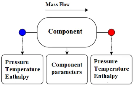
4.4.1 Standard quantities
The standard quantities are depicted on Figure 4-1. For each component, inlet and outlet quantities are available (pressure, temperature, enthalpy).
Figure 4.1 Standard quantities
The mass flow passing through the component and component parameters are also available. Moreover it is included for each dynamic component a set of relationships to reproduce the transient phenomena (inertia, transfer functions, settling times) and another set of control laws in order to regulate the ECS System actuators as required through ECS system targets within the limit of available Electrical Power.
4.4.2 Component parameters
For the ECS system, the main performance components are turbomachines, heat exchangers, valves, sensors: they have a set of parameters (numerical values are encrypted), described as follows:
Turbomachine
The turbomachines represents components likes compressor, turbine or fan. The following table describes the main performance parameters of these components. The
inertia ( ) will limit the rotating speed accelerations and decelerations as identified through real tests performed similar components.
Table 4.2 Turbomachines parameters
Heat Exchanger
The heat exchangers are mainly defined by their efficiency and their response time:
Table 4.3 Heat Exchanger parameters
Valves
The valves are defined by their efficient area when fully open and their maximum angular speed during the transient phase:
Table 4.4 Valves parameters
5 Global Thermal A/C Architecture
AMESim model 5.1
5.1.1 Model description
The model is developed using the Gas Mixture, Signals and Controls, Mechanical,
Thermal, Moist Air libraries; its architecture is composed by the following sub-models,
each one of them identifying a particular zone of the aircraft:
Flight deck Avionics bay Passenger cabin Cargo compartment Under-floor Galley Lavatory
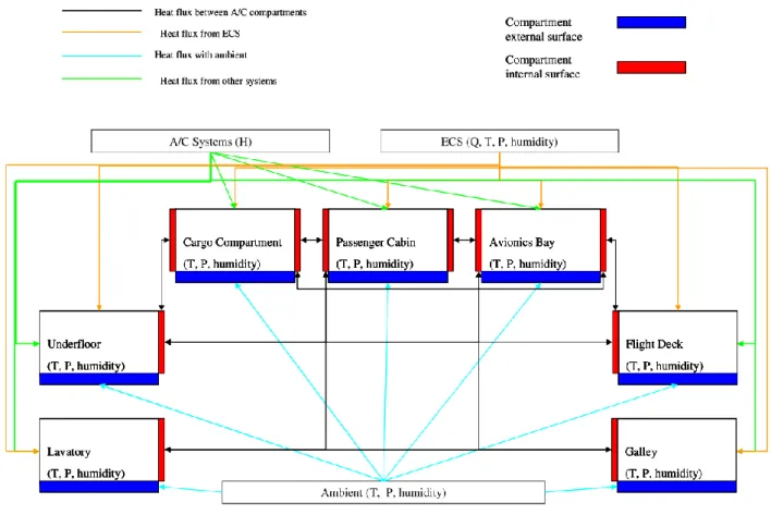
Each zone is modeled considering two aspects: the air volume enclosed and the walls effects. The first one is responsible for the computation of the hygroscopic-thermal balance, the second one for the computation of heat transport through the A/C compartment walls (both opaque and transparent walls). Finally, the model needs information about the external ambient conditions to work properly; so there is included another sub-model, which provides the necessary parameters (temperature, pressure, humidity, solar radiation) depending on A/C flight phase (velocity, altitude) and weather data (ISA day). As shown in the following figure each zone model is linked with:
other zone models
ambient model
ECS model
Figure 5.1 Thermal Architecture Model
Ambient model
The ambient model has the following inputs: 1. ISA day
2. Aircraft altitude 3. Aircraft speed
The ambient model produces as output ambient temperature, ambient pressure, aircraft Mach and solar heat flux (dependent on aircraft altitude). In particular a look-up table is defined for the computation of solar heat flux:
Figure 5.2 Solar radiation intensity vs. aircraft altitude (MIL-E-38453A)
External opaque walls model
The external walls model represents the aircraft skin and thermo-acoustic panel defining the boundary between each compartment and the ambient. It is characterized by a thermal conductibility measured in and an exchange surface measured in . Skin‟s temperature is performed as follows:
If Mach number is greater than zero
where both temperature are expressed in kelvin.
Otherwise (A/C on ground), if the ambient temperature is above 0°C, the external skin temperature is evaluated as:
where the numeric value “1.238” considers in a simplified way the solar radiation effects on A/C skin temperature. If the user wants a more precise evaluation of this aspect it is necessary to solve iteratively the equation of thermal balance of a plate with absorptivity subject to solar radiation:
Finally, in case of A/C on ground and ambient temperature below 0°C, is assumed equal to .
Internal opaque walls model
This model represents the aircraft internal partition panels defining the boundary between different A/C internal compartments and the external ambient. It is characterized by a thermal conductibility measured in and an exchange surface measured in .
Transparent walls model
The model represents the aircraft windows defining the boundary between compartments and the external ambient. It is characterized by a thermal conductibility measured in and an area (window projected area) measured in .
5.1.2 Parameters and interfaces
The user can define internal parameters such as A/C compartments geometrical definition (volume, internal and external surface), A/C compartments walls (both opaque and transparent), passenger cabin occupants number, flight deck occupants number. De facto all these data are inputs to the model.
Concerning the interfaces, the table below highlights a preliminary estimation of the required external data:
Sub-model External interfaces External model
Ambient model ISA day SSE Input
External hygrometric data A/C velocity
A/C altitude
Zone model Air conditioned mass flow ECS model
Air conditioned temperature Air conditioned hygrometric data
Air conditioned pressure
Heat load Utilities model
Heat load Avionics
Heat load EPGDS model
Table 5.1 Thermal Architecture Model external interfaces
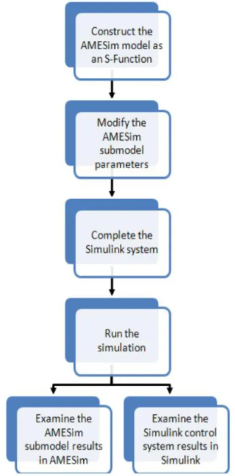
AMESim – Simulink Interface 5.2
This particular feature of the software gives the user the possibility to construct a model in AMESim, convert it to a Simulink S-Function and then use it as usual, with the block
“S-Function”, in the Simulink library, section User-Defined Functions, according to the
figure 5.4.
But the user has another choose, i.e. he can use another type of interface, called Co-Simulation, which gives the possibility to run the Co-Simulation itself between Simulink and AMESim.
The two interfaces are designed so that the user can change parameters directly in AMESim before running a simulation or use many of the software‟s facilities while the simulation itself is running.
Figure 5.3 AMESim – Simulink Interface
5.2.1 Preliminaries
First of all a C compiler has to be necessarily installed, to create the S-Function; the only one supported by Simulink is Microsoft Visual C++ (2010 version is compatible with the other software versions used). The first time the user uses the interface, each time a new compiler or a new version of Matlab is used, he must type on the Matlab command window “mex –setup” and follow the instructions, to configure the compiler. Even in AMESim environment the compiler‟s setup has to be done (from the menu Tools->Options-> AMESim Preferences->Compilation).
menu “Modeling -> Interface block -> Create interface icon”. The dialog box is shown in figure 5.5:
Figure 5.4 Interface Icon Creation dialog box
The number of inputs and outputs can be increased or decreased by selecting the arrow buttons in the top corner, considering a reasonable upper limit, e.g. 10. Otherwise it is better to use more than one interface block. Blank spaces are useful to give (from left to right) a label to the input variables, a description of the model and a label to the output variables. It is worth mentioning that input and output to and from Simulink cannot be vectors and if there are more than one interface blocks in the AMESim model, they must all be of the same type: indeed selecting the sub-menu “Type of interface” the user has many available choices. In particular the “Simulink” option gives the possibility to create a stand-alone model, while the “SimuCosim” allows to use the Co-simulation mode between the two software involved, as said before. At this point, once the sketch of the model is complete, the user can select the Submodel mode and then the
Parameter mode, to complete the process. An example of interface block, used to test
Figure 5.5 AMESim Interface Block
Now, selecting the Simulation mode (the first button under Parameter mode) the user has the possibility to lunch Simulink directly and the path is automatically set where the
.ame file is located (very important for Simulink, to find the S-Function). At this point
the user can import the AMESim model: selecting the block S-Function and double clicking on it, a dialog box will appear:
software help manual. A more fast and accurate way to import the model can be used
when is defined a Co-Simulation interface block, just typing
amecreatecosimsfunmask(„systemName‟, ‟amename‟) in the Matlab command window.
(note that it works only if Matlab is opened from AMESim). Indeed in this case there are more than two parameter to be set, e.g interval communication between the two software, print interval in AMESim, relative tolerance of the solver, global parameters in the AMESim model, integration step for a fixed step solver and so on. More information can be found in the software‟s help manual. The main differences between the “Simulink” and “SimuCosim” interface block (and all the differences about simulation) are treated later. At this point the user can complete his Simulink model and then run a simulation. Finally it is important to underline that the inputs of the Interface block become the outputs of the Simulink block and the outputs of the Interface block become the inputs (the enumeration of these one is even reversed) as shown in the following figure:
Figure 5.7 Simulink S-Function block associated to the AMESim model
Encryption of an AMESim model 5.3
The encryption of a model has two main purposes:
opening it accidentally in AMECustom (an environment that gives the possibility to modify and customize a model). This is the role of the password, necessary to open any encrypted customized object.
Protect the Intellectual Property (IP) stored in the customized object from any reverse engineering operations. This is especially true when the customized objects are sent to third-party users.
Referring to the previous section of this chapter, it is worth mentioning that an interface block cannot encrypted. So, for this reason, the entire Global Thermal A/C Architecture is enclosed into an AMESim Supercomponent, that is an icon that includes the model, with inputs and outputs, as displayed in the following figure:
Figure 5.8 Supercomponent in AMESim
Now the user has to open the Supercomponent. Referring to the following dialog box, he has to click on the button circled in red. In this way the tab Category Saving will appear. At this point it is possible to create a new category that will appear in the library tree or select an existing one (section circled in blue). The other section (circled in
Figure 5.9 Supercomponent dialog box
The next step is to run AMECustom, open the model just saved (it is a .spe file) and save it selecting the option Save encrypted:
Figure 5.10 Encryption of a Supercomponent
A password has to be set by the user as it is visible in picture 5-11 to encrypt the model and to modify it. It is important that compiler‟s options are identically set in AMESim
and AMECustom otherwise some errors can occur at the compilation instant. Moreover the correct value (compiler‟s installation directory) of the environment variable “include” has to be checked.
While the software is compiling the model, it can ask to include some .data or .txt file used to create the model; the user has only to indicate the correct path.
The files created with the entire process and useful to send a model to a third part are:
.c
.lib
.spe (Included in …/submodels directory)
.sub (Included in …/submodels directory)
.des.tmp (Included in …/submodels directory)
.spe.bak (Included in …/submodels directory)
.sub.bak (Included in …/submodels directory)
.lib (Included in …/win64 directory)
.obj (Included in …/win64 directory)
The name of the last subfolder depends on the compiler‟s settings (in this case a 64bit compiler).
Linear Analysis of the model 5.4
The Simulink tool called Linear Analysis gives the possibility to linearize a complex model around an equilibrium point (Operating point). The goal is to found the behavior, and so the transfer function, between the cabin temperature and the temperature target to send to the ECS, in order to develop the correct control law, as described in chapter 7. The exchanged heat flow between the two systems can be written as follows:
∫ ̇ We now want to arrive at the same result using the Linear Analysis tool. So, the first thing to do is setting all the environment temperature ( ) and pressure ( ) of the model at the same value, ignore the term, i.e. set to zero the electrical cabin loads, the number of passengers, the heat exchange between the cabin and the external environment, the two fans action and the solar radiation. If we now send an air flow of from the ECS (at the same temperature and pressure), we can see how the system finds an equilibrium position, after an initial short transient, around its initial conditions, in about 2000 seconds. So, this is the Operating point found via dynamic simulation, which is called Snapshot in the Linear Analysis tool. Linearizing the model around this point we found what we expected, as it is clearly visible in figure 5.12 and 5.13:
Figure 5.12 Bode diagram ( )
Analyzing the transfer function structure, it has 43 poles and 40 zeros, but the most import dynamic, which is a first order type, is given by a real pole of about 0.004; indeed the constant time (blue point in figure 5-12) is at 953 seconds. These open loop results will be useful for the closed loop analysis.
6 Simulation Analysis
Simulink Environment 6.1
Once the Global Thermal Model is imported into the Simulink SSE scheme, the next step can be done, i.e. connect it with the other models and prepare the simulation. At this point there are two different available ways:
- “Stand alone” mode - Co-Simulation mode
6.1.1 “Stand alone” mode
These words indicate the use of the Simulink block interface and it gives the user the possibility of running a simulation without opening AMESim: indeed, when the .ame file is lunched, various temporary files are created (they are canceled as soon as AMESim is closed). The user has only to copy these ones into the Simulink work directory to obtain a “stand alone” model:
- .gp - .gp2 - .data
- .mexw64 (or .mexw32 depending on the compiler‟s settings) - various .txt files containing data used in the model
At this point a simulation run can be done, with the constraint to choose only one Simulink solver; it is important, indeed, to underline that a lot of AMESim systems are numerically stiff that can require even more than one variable step solver. AMESim is able to do this operation because it can change the solver while a simulation is running.
where y is the variable state vector. Solving or integrating the equations means determining how this vector changes as the time t progresses from 0 to .
One way of analyzing the characteristics of the equations at a generic point is to evaluate the Jacobian matrix J and determine its eigenvalues , which are, in general, complex with real parts normally negative. Of interest to the engineer are the corresponding time constants, defined as follows:
Problems where are called stiff and require very stable methods for efficient solution.
In Simulink there are two type of solvers: - fixed step
- variable step
Preliminary tests were done on each system present in the SSE scheme to evaluate the best solution using both type of solvers; the results are summarized in table 6.1:
Table 6.1 Preliminary tests - Computational times
Fixed step Variable step
Solver Computatio n time per 3 seconds of simulation Solver Computation time per 3 seconds of simulation Method Integratio n step Method Relative tolerance Min. step size ECS Runge -Kutta (4) 10 -7 ~ 1h 30’’ ode15s (stiff/NDF) 10 -3 10-3 few seconds Dormand-Prince(5) 10 -7 ~ 1h 30’’ ode23s (stiff/Mod. Rosenbrock) 10-3 10-3 few seconds Dormand-Prince(8) 10 -7 ~ 2h’
ode23tb 10-3 10-3 few seconds
FCS Runge –
Kutta (4) 10
-3
few seconds none - - -
LGS Runge – Kutta (4) 10 -3 few seconds ode113 (Adams) 10 -3 10-7 few seconds ode23s (stiff/Mod. Rosenbrock) 10-3 10-7 few seconds ode23t (mod. stiff/Trapezoidal ) 10-3 10-7 few seconds CT Runge -Kutta (4) 10 -7 ~ 1h 30’’ ode15s (stiff/NDF) 10 -3 10-3 few seconds Dormand-Prince(5) 10 -7 ~ 1h 30’’ ode23s (stiff/Mod. Rosenbrock) 10-3 10-3 few seconds Dormand-Prince(8) 10 -7
6.1.2 Co-Simulation mode
The main differences with the previous described simulation mode are two: the first is the usage of two (or more) solvers: this means that each platform uses its own during the simulation run. The second is that the AMESim block is not seen by Simulink as a continuous, but as a discrete system: so the user can set a Sample Time, useful to exchange data between the two software.
Figure 6.1 AMESim – Simulink interfaces
As it is visible in this figure with the Normal interface the AMESim part of the system gets state variables and input variables from Simulink and calculates state derivatives and output variables. The entire process is controlled by the Simulink solver, so one could say that the equations are imported into Simulink. Instead, with the Co-simulation
interface only inputs and outputs are exchanged so the entire model is not completely
controlled by one software. It is important to notice that this exchange of data could generate a loss of information if the Sample time is not appropriately set. Obviously the smaller value is used, the closer to the continuous model is obtained. Finally during a simulation run of this type, both software (AMESim and Simulink) have to be lunched). When the user wants to create a Co-Simulation interface from the AMESim menu, the dialog box is the following:
Figure 6.2 Interface Icon Creation dialog box
The only difference, noticeable comparing this figure with the 5.5, is the Type of
interface. At this point the user can import the model into Simulink using the S-function
block or the command amecreatecosimsfunmask as said before. Using the last, an example of dialog box is the following:
The meaning of each parameter is explained in table 6.2:
Table 6.2 Co - simulation parameters - explanation
Simulation Parameters in Simulink 6.2
Once Co-Simulation is found to be the best way to operate with two (or more) software, the choice of the right solver and the setting of the other parameters is essential to obtain both good results and good computational time. We have to say that when it is necessary to simulate a large engineering system, it is normal to reduce any partial differential equations to ordinary differential equations. This leads to models with either ordinary differential equations (ODEs) or differential algebraic equations (DAEs). A generic solver is a tool that applies a numerical method to solve this set of ordinary differential equations that represent the model; it also satisfies the accuracy required by
the user.
Simulink gives the possibility to choice between two type of solvers: - fixed-step solver
- variable-step solver
Both fixed-step and variable-step solvers compute the next simulation time as the sum of the current simulation time and a quantity known as the step size. With a fixed-step solver, the step size remains constant throughout the simulation (defined by the user). In contrast, with a variable-step solver, it can vary from step to step, depending on the model dynamics. In particular, a variable-step solver automatically increases or reduces the step size to meet the error tolerances that the user specify: for this reason it can drastically reduce computational times. Even if a variable step solver could appear the best solution, the choice of the right solver depends on other aspects: for example generate code from a model and then run it on a real-time machine requires a fixed-step solver.
Some preliminary tests were done to choose the best solver, using both types and comparing the obtained results. In particular the Simulink model used includes the blocks Mission profile, Engine, FCS, LGS, ECS, CT (the EPG_Voltage is set as constant value of 270V). It is the following:
Figure 6.4 SSE – preliminary tests
The chosen solver is the ode23t and the obtained computational times (using an HP Z800 Workstation, dual-processor, 64 bit, six-core system), that will be kept even in the complete SSE, are about five seconds for one second of mission.
It is a variable-step solver and it can be included in the category of one-step solvers: the Simulink solver library indeed, provides both one-step and multistep type. The first one estimate using the solution at the immediately preceding time point, , and the values of the derivative at a number of points between and . These points are minor steps. The multistep solvers use instead the results at several preceding time steps to compute the current solution.
Some considerations must now to be done about the accuracy for a solver of this kind, so we have to introduce the concept of error and tolerance. About the first one, in particular a local error, the variable-step solvers use standard control techniques to monitor it at each time step. During each time step, the solvers compute the state values at the end of the step and determine the local error; it is the estimated error of these state values ( ). They then compare the local error to the acceptable error, which is a function of both the relative tolerance ( ) and the absolute tolerance ( ). If the local error is greater than the acceptable error for any one state, the solver reduces the step
size and tries again. The relative tolerance measures the error relative to the size of each state; it represents a percentage of the state value. The default value is set to 0.001. The absolute tolerance is instead a threshold error value and it represents the acceptable error as the value of the measured state approaches zero. It is applied to all states in a model.
The solvers require the error for a generic state, to satisfy: | |
The following figure shows a plot of a state and the regions in which the relative tolerance and the absolute tolerance determine the acceptable error.
Figure 6.5 Absolute and Relative tolerance
Simulink sets the absolute tolerance for each state to 1 as default value. As the simulation progresses, the absolute tolerance for each state resets to the maximum value that the state has assumed so far, measures the relative tolerance for that state. Thus, if a state changes from 0 to 1 and is 1 , then by the end of the simulation, becomes 1 also. If a state goes from 0 to 1000, then
changes to 1.
A too low value for absolute tolerance causes the solver to take too many steps in the vicinity of near-zero state values, so the simulation is slower. On the other hand, a too high can be inaccurate as one or more continuous states in your model approach zero. So once the simulation is complete, the user can verify the accuracy of the results by reducing the absolute tolerance and running the simulation again. If the results of these
Figure 6.6 AMESim simulation parameters
In the previous figure there are highlighted the Standard options related to the standard AMESim integrator, which is a variable-step one. The approach is very different from Simulink because it is clear that the user cannot choose a specific solver and so a specific numeric algorithm. This is reasonable if you understand the AMESim philosophy: even for an experienced numerical mathematician could be very difficult to choice a valid algorithm because the characteristics of the equations may change during the simulation‟s process. So, for this reason AMESim is able to change the solver while the simulation is running to optimize the solution (for the differential equations) and the computational times. So the user can completely dedicate his attention to the model. If the software detects the presence of implicit variables, the solver used is the DASSL. Instead, if the system of equations is purely odes AMESim uses Gear‟s method for stiff problems or LSODA for non-stiff problems.
7 Cabin Thermal Model: Closed Loop Analysis
While the A/C is performing its mission it is important to guarantee optimal conditions for the passengers in the cabin in terms of temperature and pressure. So, for this reason, it is necessary to put the model in closed loop to obtain preset values of these two magnitudes.
Temperature controller 7.1
To better understand we can consider the following “retroaction-scheme”:
Figure 7.1 Retroaction scheme
where is the required temperature value in the cabin and its difference with the actual cabin temperature ( ) is processed by the controller. The magnitude comes out from this block is the target temperature for the ECS system, obtained by the relation:
( ) where k is the generic controller gain. Depending on the value of the ECS target, the
system regulates the air temperature that must be sent into the cabin.
Analyzing more in detail the block called “CONTROLLER” we can find a proportional integrative derivative controller (PID) as the best solution. In formal way we have:
- +
The various values of gains, zeros, and poles were founded observing different tests done on the global model. About the proportional gain we can say that if i.e. the actual cabin temperature is minor than the target value, the ECS must provide a “hotter” quantity of air to the cabin, so must be greater than zero. The same line of reasoning can be used if . Concerning the integrative part of the controller, it is used to reduce the error when the system operates at full speed; on the other side the derivative part was used to reduce the overshoot and to introduce more damping into the system. We have to underline that in the controller implementation (Simulink) it was not used the derivative block, that can be found in the Continuous section of the Simulink library, because the temperature signal is discrete due to the co-simulation process. So the derivate part is deduced from
where is the temporal interval used for the co-simulation between AMESim, Simulink and Dymola.
The gain values used for the controller are:
-
-
-
In a formal way, the transfer function controller can be written as:
( ) Using the SISO Matlab tool is possible to see the root locus when this controller is applied to the transfer function , which is a first order, as it was been described in chapter 5. The entire transfer function is:
( )
where there is an electronic pole settled into the origin and two zeros, with value:
The root locus is:
Figure 7.2 Temperature controller: Root Locus
The figure describes the closed loop position for the poles of the system (CT transfer function, and PID controller): changing the closing gain the system can be a first or a second order type. Using a stronger derivative action (allocating the zero closer to the origin), more damping can be introduced in the system. More tests can be done to optimize this aspect, even because the ECS dynamic is not known (model encrypted).
Pressure controller 7.2
The pressure value of the cabin is very important because the quantity of oxygen in the
-10 -9 -8 -7 -6 -5 -4 -3 -2 -1 0 x 10-3 -2.5 -2 -1.5 -1 -0.5 0 0.5 1 1.5 2 2.5 x 10⁻³ Root Locus
Real Axis (seconds-1)
Im a g in a ry A x is ( s e c o n d s -1 )
Pressure control is made using the so called outflow valves: they are put in the low part of the fuselage and they act on the air flow rate coming in the cabin, indeed a too much high pressure causes the opening of the valve and the exit of the exceed air, instead a too much low value causes the closing and the increase of the cabin pressure. An example can be seen in the following picture :
Figure 7.3 Boeing 737-800: outflow and relief valve
The original Cabin Thermal Model implemented in AMESim had the following target pressure:
where is evaluated in bar, and (A/C altitude) in feet.
Considering the controller implementation it creates a sort of virtual cabin altitude, which is different by the A/C mission altitude and that establishes the cabin pressure. The AMESim component used is a simple butterfly valve.
7.2.1 Pressure controller with butterfly valve
Figure 7.4 Pressure controller with butterfly valve
In the previous pictures is visible the changes done in the AMESim model: starting from the upper right corner we can see the violet pressure source that sends the pressure target (the one comes from the virtual cabin altitude) to the butterfly valve, enlightened in the green region, which represents the low part of the fuselage. The AMESim component needs two input, i.e. the pressure target (red circle) and the command law (sky blue one). The last one is implemented in Simulink with a simple proportional gain and indicates the opening angle valve:
[ ( )]
The error between the target and the actual value is multiplied by the gain (value of 45), then is converted into degrees (limited to 90°) and sent to the valve. We can observe
Evaluating the obtained results we can see how the maximum of project (8-9 psi or ~0.055 MPa) for A/C of civil aviation with reaction propulsion), that is the maximum difference between the external pressure and the cabin one, is not overtaken. If this event occurs with a different A/C mission, the controller must be slightly modified, in other words the presence of a relief valve must be introduced.
8 Energy Management System
During the A/C mission, a generic extra electrical load can occur; so, it is completely addressed to the overload capacity of the generator. This circumstance can be very dangerous if this load is too high, so, the introduction of the EMS becomes indispensable: it is a set of logics used for the optimal sharing of the total on-board electrical power, indeed, in some mission sections, several loads may be totally shed or temporary reduced, because they are not flight or safe-landing essential. Thus no overload can be found because this set of specific control laws, acting on power electronics and motor controllers, change the supplied power to each system with respect to the requested one. The model is implemented in Dymola (encrypted) but not in its final version; at the moment, indeed, all the control strategy is not implemented.
EMS Supervisory Control Strategy 8.1
We want to describe now the high-level control algorithm embedded within the EMS is described, as shown in figure 8.1:
It is visible in the top of the picture that the generator total current derivative ( ) is the first important parameter: it can predict in some way the entity and the type of transient overload condition, in order to obtain a more or less (strongly decrease or decrease) strong power modulation via SSPCs (switching contactors high frequency modulated, connected to the resistive loads), operating on their duty cycle ( ).
The algorithm starts from the black block on the top, where we can find steady state conditions, i.e. when SSPCs are completely “closed” (duty cycle=1) and the ECS operates at nominal power for that specific flight phase. Moreover the generator current ( ) is always monitored. As soon as a certain threshold is overtaken, a watchdog is activated and the duty cycle reduction is activated. If the overload situation is persistent, sequentially the SSPC reaches the minimum duty cycle, below which the connected equipment functionality is declared unacceptable. If all the SSPCs reach this condition, the only solution is to act on the ECS, with the attention put on the Cabin Temperature: if its value is below a certain threshold, the successive action is the lowest priority load shedding, which depends on a specific flight phase.
Because the ECS operates only if all the SSPCs have reached the minimum value, its intervention is meant to be “asynchronous” with respect to the EMS strategy.
At the moment all this strategy is not implemented and the Dymola block simply pass throughout the generator voltage (270 V).
Dymola – Simulink Interface 8.2
This interface consists of some .m files which are a set of Matlab utilities and a Simulink block, called DymolaBlock which allows to import a Dymola model once the user has defined inputs and outputs. In order to use all these features the first operation to do is include the following directories in the Matlab path:
Program Files\Dymola 2013 FD01\Mfiles
Program Files\Dymola 2013 FD01\Mfiles\dymtools
Program Files\Dymola 2013 FD01\Mfiles\traj
The user has to pay attention when he uses the Matlab command restoredefaultpath because it restores the original path and removes these previous added ones. Moreover the only compiler who consents to generate the S-function is Microsoft Visual C++ (version 2010 is well-matched with the other software used). Finally note that Matlab
R2010bSP1, R2011a, R2011b, and R2012a will give warnings that files in the Program
Files\Dymola 2013 FD01\Mfiles folder are generated with an old p-code version. These
warnings are uncritical and can be turned off by adding the following line to the Matlab startup script:
warning('off', 'MATLAB:oldPfileVersion')
The way to import a generic Dymola model into Simulink is much closer to what it was explained about AMESim: the DymolaBlock is indeed a shield around an S-function MEX block, i.e., the interface to the C-code generated by Dymola. By double-clicking on the block a graphical user interface is opened to configure everything is necessary for the compilation. As it is visible in the following picture it is important to set the Model
name and File name; a fast way is to open the desired model in Dymola, let the program
opened and then click on the button Select from Dymola. The button Edit model allows to modify a Modelica model (Modelica is the language used by Dymola), Reset
Parameters restore parameters and start values to the default in Dymola, Compile model
9 Simulation Run and Results
Initial trim procedure 9.1
Once the SSE is complete in its prototype version, it is possible to obtain the first numerical results. This tool is designed to simulate typical A/C manoeuvres starting from assigned initial trim conditions, where the various systems can be characterized by not null currents and by constant values of the internal variables and states. An off-line evaluation (before starting the simulation) of the trim would have been complex, so it is done via a dynamic simulation, made within and additional initial time: a time range of 150 seconds is added at the beginning of the time histories, as schematically described in figure 8-1. In this time range, each input variable is kept constant and equal to its first value in the time history. Moreover, to reduce the computational time during this phase, the various involved models are progressively enabled with the following sequence:
- EPGS and EMS at the beginning - FCS and LGS start at 10 seconds - ECS at 20 seconds
- CT model and its controller at 30 seconds
This approach, based on the progressive enabling, drastically reduces also the possibilities of incurring in the divergence of some systems during the trim-search phase.
Figure 9.1 Time range added to evaluate the trim condition via dynamic simulation
At this point the user can choose two different type of flight histories, and therefore two different type of input data.
input t input t original modified 150 sec
Time range added to let the systems reach the “trim”
“Dummy” input data 9.2
The user has to choose between two different input data for the simulation: the first is not a real flight history and it is used to evaluate the dynamic behavior of each system being part of the SSE. Indeed the altitude and the Mach number are set to a constant value (respectively 0 and 0.38), the angle of attack, the angle of sideslip, the Euler Angles, the angular velocities and the angular accelerations are all set to zero. Instead the deflection range of all control surfaces is arbitrary between the minimum and the maximum and the engine is at full operative speed. The total “flight history” time is , where the first are used to trim the model, in particular the ECS and the Cabin, as said before. There is a request of decreasing temperature at and the activation of the landing gear system few seconds after the trim procedure. The most important input are reported in figure 9.2 and 9.3:
Figure 9.3 “Dummy” input data – Control Surfaces Deflection
Simulation results (CPU time 43 min, 28.902 seconds) are summarized in the pictures from 9.4 to 9.12:
Figure 9.4 “Dummy” results – Control Surfaces Deflection
0 50 100 150 200 250 300 350 400 450 500 0
10 20
LEFT AILERON Angular Deflection
time [s] [d e g ] Reference Actual 0 50 100 150 200 250 300 350 400 450 500 -20 -10 0
RIGHT AILERON Angular Deflection
time [s] [d e g ] Reference Actual 0 50 100 150 200 250 300 350 400 450 500 -20 0 20
LEFT ELEVATOR Angular Deflection
time [s] [d e g ] Reference Actual 0 50 100 150 200 250 300 350 400 450 500 -20 0 20
RIGHT ELEVATOR Angular Deflection
time [s] [d e g ] Reference Actual 0 50 100 150 200 250 300 350 400 450 500 -20 0 20
RUDDER Angular Deflection
time [s] [d e g ] Reference Actual 0 50 100 150 200 250 300 350 400 450 500 0 5 10
LEFT INBOARD FLAP Angular Deflection
time [s] [d e g ] Reference Actual 0 50 100 150 200 250 300 350 400 450 500 0 5 10
RIGHT INBOARD FLAP Angular Deflection
time [s] [d e g ] Reference Actual 5 10
LEFT OUTBOARD FLAP Angular Deflection
[d e g ] Reference Actual
Figure 9.6 “Dummy” results – LG Extraction/Retraction
Figure 9.7 “Dummy” results – EPGS Voltage and Current
0 50 100 150 200 250 300 350 400 450 500
0 0.5 1
Nose EMA rod position
time [s] [m ] Actual Reference Activation 0 50 100 150 200 250 300 350 400 450 500 0 0.5 1
Left EMA rod position
time [s] [m ] Actual Reference Activation 0 50 100 150 200 250 300 350 400 450 500 0 0.5 1
Right EMA rod position
time [s] [m ] Actual Reference Activation 0 50 100 150 200 250 300 350 400 450 500 0 100 200 300 EPGS time [s] E P G S v o lt a g e ( V ) 0 50 100 150 200 250 300 350 400 450 500 0 100 200 300 time [s] E P G S c u rr e n t (A )
Figure 9.8 “Dummy” results – ECS Outlet Temperature and Mass flow 0 50 100 150 200 250 300 350 400 450 500 -200 -100 0 100 200 time [s] P a c k O u tl e t te m p e ra tu re ( °C ) ECS Actual Target 0 50 100 150 200 250 300 350 400 450 500 0 0.5 1 1.5 time (s) P a c k O u tl e t m a s s f lo w (k g /s ) 0 50 100 150 200 250 300 350 400 450 500 0 10 20 30 40 time [s] C a b in T e m p e ra tu re ( °C ) CT Actual Target 1.1 1.15 re (b a r) Actual Target