Alma Mater Studiorum – Università di Bologna
DOTTORATO DI RICERCA IN
Dottorato in Ingegneria Civile, Ambientale e dei Materiali
Ciclo XXVII
Settore Concorsuale di afferenza: 08/B1 Settore Scientifico disciplinare: ICAR/07
Statistical analysis of the error
associated with the simplification of
the stratigraphy in geotechnical models
Presentata da: Giulia Bossi
Coordinatore Dottorato Alberto Lamberti Relatore: Guido Gottardi Co-relatori Lisa Borgatti Gianluca Marcato
“Essentially, all models are wrong, but some are useful” George Edward Pelham Box (1987)
Abstract ... 1
Sommario ... 3
1 Introduction ... 5
1.1 Sources of uncertainties ... 6
1.2 Spatial variability in natural soils ... 6
1.3 Approaching uncertainty in geotechnics ... 7
1.3.1 Inherent soil variability and measurement errors ... 8
1.3.2 Data scatter ... 8
1.3.3 Geotechnical models that account for uncertainty ... 9
2 Tools and Method ... 11
2.1 Tools... 11
2.1.1 FLAC ... 11
2.1.2 MatLab ... 11
2.1.3 Monte Carlo methods ... 12
2.1.4 Random numbers generation... 12
2.2 Method ... 13
2.2.1 Boolean Stochastic Generation method - BoSG ... 13
2.2.2 The computational algorithm ... 14
2.2.3 2D algorithm ... 15
2.2.4 3D algorithm ... 18
3 Simple applications ... 21
3.1 2D - Simple slope with horizontal layering ... 21
3.1.1 Soil deformations ... 21
3.1.2 Spatial uncertainty ... 26
3.2 3D - Simple slope with horizontal layering ... 28
4.1 Study area ... 35 4.2 Geology ... 36 4.3 Stratigraphy ... 38 4.3.1 1989 investigations ... 38 4.3.2 1991 investigations ... 39 4.3.3 2009 investigations ... 40
4.4 Geomorphological evolution of the Mortisa landslide ... 42
4.5 Monitoring network ... 50
4.5.1 GNSS benchmarks ... 50
4.5.2 Inclinometers on Sector 2 ... 52
4.6 Geotechnical lab tests ... 56
4.7 BoSG modeling ... 60
4.7.1 Definition of the cross section... 60
4.7.2 Definition of the mesh geometry... 61
4.7.3 Definition of first trial soil parameters ... 62
4.7.4 BoSG simulation with first trial soil parameters ... 62
4.7.5 Analysis with interval modeling – Point Estimate Method (PEM) . 69 5 Conclusions ... 81
1
Abstract
The uncertainties in the determination of the stratigraphic profile of natural soils is one of the main problems in geotechnics, in particular for landslide characterization and modeling. The study deals with a new approach in geotechnical modeling which relays on a stochastic generation of different soil layers distributions, following a boolean logic – the method has been thus called BoSG (Boolean Stochastic Generation). In this way, it is possible to randomize the presence of a specific material interdigitated in a uniform matrix.
In the building of a geotechnical model it is generally common to discard some stratigraphic data in order to simplify the model itself, assuming that the significance of the results of the modeling procedure would not be affected. With the proposed technique it is possible to quantify the error associated with this simplification. Moreover, it could be used to determine the most significant zones where eventual further investigations and surveys would be more effective to build the geotechnical model of the slope. The commercial software FLAC was used for the 2D and 3D geotechnical model. The distribution of the materials was randomized through a specifically coded MatLab program that automatically generates text files, each of them representing a specific soil configuration. Besides, a routine was designed to automate the computation of FLAC with the different data files in order to maximize the sample number.
The methodology is applied with reference to a simplified slope in 2D, a simplified slope in 3D and an actual landslide, namely the Mortisa mudslide (Cortina d’Ampezzo, BL, Italy). However, it could be extended to numerous different cases, especially for hydrogeological analysis and landslide stability assessment, in different geological and geomorphological contexts.
3
Sommario
L’incertezza nella determinazione del profilo stratigrafico e dei parametri meccanici dei singoli terreni è tra i principali problemi dell’ingegneria geotecnica, in particolare per l’analisi dei fenomeni franosi.
Lo studio presenta un nuovo approccio nella modellazione geotecnica che si basa sulla generazione stocastica di diverse distribuzioni di strati di terreno, seguendo una logica booleana - il metodo è stato perciò chiamato BoSG (Boolean Stochastic Generation – Generazione Stocastica Booleana). Con questo metodo è possibile randomizzare la presenza di uno specifico materiale interdigitato in una matrice uniforme.
Nell’impostare un modello geotecnico, infatti, generalmente si eliminano alcuni dati stratigrafici per semplificare il modello stesso, assumendo che la significatività dei risultati non ne risenta. La metodologia proposta permette di quantificare l'errore associato a questa semplificazione. Inoltre, può essere utilizzata per determinare le zone più significativi nelle quali possibili ulteriori indagini geotecniche sarebbero più efficaci per la definizione del modello geotecnico. Per la modellizzazione bidimensionale e tridimensionale è stato utilizzato il software commerciale alle differenze finite FLAC. La distribuzione dei materiali è stata randomizzata attraverso un programma in MatLab specificamente codificato che genera automaticamente dei file di testo con le configurazioni del terreno. E’ stata inoltre programmata una routine per automatizzare il calcolo FLAC con diverse file di dati al fine di massimizzare la numerosità campionaria.
In questa tesi la metodologia è stata applicata ad un pendio semplice in 2D, un pendio semplice in 3D e una frana reale: la frana di colata di Mortisa (Cortina d'Ampezzo, BL). Il metodo, tuttavia, potrebbe essere applicato ad altri casi, in particolare per studi di idrologia sotterranea, per l’analisi di stabilità di altre frane e in diversi contesti geologici e geomorfologici
5
1 Introduction
Quantifying uncertainty and reliability is one of the main problems in engineering (Whitman 2000). Among engineering fields geotechnics is atypical as most of the times it deals with materials whose properties and spatial distribution are not well known (Baecher & Christian 2005). Accounting for all the uncertainty could lead to unpractical and uneconomical technical designs (Beer et al. 2013), therefore, since the dawn of the discipline proper methods or useful turnarounds have been proposed to solve the problem.
Many of the most influential researches of geotechnics approached uncertainty as a fundamental issue for the field. In 1929 Terzaghi (Terzaghi 1929) proposed the use of a combination of analogies with prior projects and continuous monitoring during construction in order to adjust design to the influence of uncertainties. Casagrande (Casagrande 1965) introduced the term “calculated risk” introducing probability theory to account for uncertainties in a field that was prior focused only deterministic methods. In 1969 Peck (Peck 1969) expands the Terzaghi concept of “learn as you go” that will be then known as observational method.
It has been said (Christian 2004) that the observational method is related to the techniques of Bayesian updating since it reduce uncertainty on the basis of previous analysis. In this framework, we can also insert back analysis methods (Gioda & Sakurai 1987) like the ones used for landslide characterization and modeling.
Back analysis has been broadly used despite its intrinsic limitations (Leroueil & Tavenas 1981). In the review of Deschamps & Yankey (2006) the main issues are listed and they comprise: the problem of back analyze the actual slip surface and with reliable pore pressure data, three dimensional effects and the relative strength of materials in heterogeneous profiles.
In this work we will introduce a methodology which estimates the uncertainty linked to marked soil heterogeneity. With the proposed technique it is possible to quantify the error through the generation of different configurations and the automatic analysis of the results.
6 1.1 Sources of uncertainties
Uncertainty is the main constrain in engineering practice. It concerns (Nadim et al. 2005):
Spatial and temporal variability; Measurement errors;
Statistical fluctuations; Model uncertainty;
Uncertainty in the determination of the applied loadstriggering ; Omissions.
These types of uncertainties may be classified in two subcategories namely aleatory (or inherent or random) uncertainty and epistemic (or knowledge) uncertainty (Ang & Tang 2004; Hanss & Turrin 2010). The name of the first one origins from the Latin word alea (dice) and the concept is connected with the intrinsic randomness of the variable (Kiureghian & Ditlevsen 2009). On the other hand, epistemic uncertainty means lack of knowledge (επιστημη) or data. Different approaches have been proposed to deal with each of these uncertainties; in this work we approach epistemic uncertainty.
Epistemic uncertainty may be divided in three categories (Baecher & Christian 2005): model uncertainty, parameter uncertainty and site characterization uncertainty, in particular associated with the spatial distribution of natural soils.
1.2 Spatial variability in natural soils
“Minor geological details” (Terzaghi 1929), could have major impact on the stability of structures or slopes. For the geotechnical engineer the geometry and the properties of the materials implicated in the study usually are inferred on the basis of a small amount of data resulting from sparse information (Beer et al. 2013). For example, the uncertainty in the determination of the stratigraphic profile of natural soils is linked to the punctual nature of the typical investigation procedure, i.e. boreholes. How to expand the stratigraphy in other dimensions? In theory, knowing the spatial distribution of different geological units, their thickness, their number is of crucial importance for the matching between actual phenomena and their mathematical representation (Phoon & Kulhawy 1999). In
7
practice every engineer knows that a perfect match is unachievable and, moreover, unpractical. Geotechnical practice is thus mostly a problem of optimization largely based on induction.
In the building of a geotechnical model it is generally common to discard some stratigraphic data in order to simplify the model itself, assuming that the significance of the results of the modeling procedure would not be affected. The modeler relays mainly on expert knowledge in choosing what to dismiss and what to preserve (Kulhawy & Phoon 1996). Moreover, the distribution of some elements in the landslide body is too aleatory to be known . This leads to several problems for the modeler, as the quantification of the errors associated with the simplification of the stratigraphy is unknown. For example, if the strength parameters of the soils involved differ significantly, even a small rigid perturbation in the matrix may induce a different pattern of deformation in the slope. To address this problem many approaches have been proposed in literature, most of them relying on stochastic methods.
1.3 Approaching uncertainty in geotechnics
To date many approaches have been proposed to deal with the intrinsic aleatory character of most of the quantities (Fig. 1) used in geotechnical models (Beer et al. 2013).
8
1.3.1 Inherent soil variability and measurement errors
Uncertainties may be linked to inherent soil variability as soil is an aggregate of different materials and there may be a fluctuation of soil properties within a homogenous layer (Fenton 1999a; Heuvelink & Webster 2001). To address these problems some methods which have been proposed rely on the stochastic variation of soil parameters following a set probability function (Vanmarcke et al. 1986; Fenton & Griffiths 2002). Further research has focused on the evaluation of the Coefficient Of Variation (COV – standard deviation/mean) of soil properties (Phoon & Kulhawy 1999), or on soil anisotropy (Zhu & Zhang 2013). Other methods which account for the uncertainty of inherent soil variability follow a geostatistical approach (Vargas-Guzmán & Jim Yeh 1999; Breysse et al. 2005). However most of the times the amount of available data to is usually too small and it is not possible to infer any reliable distribution (Elkateb et al. 2003).
Stochastic method are often used to analyze data from laboratory test and field survey in order to estimate measurement errors (Kulhawy 1992; DeGroot & Baecher 1993). For this purpose random fields theory was used on CPT data to characterize the vertical variation of the analyzed soils (Fenton 1999b). Other stochastic-based methods are designed for the analysis of SPT for liquefaction susceptibility studies (Bagheripour et al. 2012) or to help defining the lithology directly in the field (Moussoutéguy et al. 2002).
1.3.2 Data scatter
Another kind of uncertainty is connected to the fact that most of the data obtained by in situ investigations, are punctual and not spatially distributed (Koike & Matsuda 2005). In fact modeling requires to formulate a hypothesis on the subsurface distribution of the soil layers relying on few stratigraphic data (Phoon & Kulhawy 1999). For this reason understanding the geological history of the investigated site may be a crucial information that would allow to decide how to approach uncertainty and select the most appropriate modeling strategy ((Christian et al. 1994; Christian 2004)). Geostatistical methods are usually used to address this problem (Deutsch 2002). Other techniques include object-based methods that have been used for modeling shales (Dubrule 1989) or to study fluvial depositional
9
processes (Deutsch & Tran 2002). Object-based methods, also known as boolean models (Baecher et al. 1977), allow approaching the sedimentary architecture of the investigated area through a chrono-stratigraphic prospective, generating facies that mimic the depositional processes.
1.3.3 Geotechnical models that account for uncertainty
Probabilistic geotechnical analysis (Griffiths et al. 2002), approach uncertainty directly in the geotechnical model, generating different distributions of soil parameters and loads in order to determine the worst-case scenario or assess the reliability of a structural work (El-Ramly et al. 2002; Breysse et al. 2007; Griffiths & Fenton 2007). Within these methods, model input parameters are assumed as random variables which can be written in the form of a probability density function.
One of the most important approaches relies on random fields theory (Vanmarcke et al. 1986) and is known as Stochastic Finite Element Method (SFEM) (Beacher & Ingra 1981).
This method is based on the spatial correlation in soil layers, which is the tendency for each soil zone to be more correlated to the closer ones than the distant ones. It addresses inherent soil variability within layers through a statistical approach (Vanmarcke 1977). In practice, a random field of soil properties is generated in a finite element mesh following an exponentially decaying spatial correlation function (Fenton & Vanmarcke 1990). Stochastic FEM may account also for uncertainties linked to measurement errors as it is usually based on experimental data (Vanmarcke 1994).
Random FEM is an evolution of stochastic FEM in which random fields are combined with FEM through a Monte Carlo simulation. In this case many soil configurations with a known mean, standard deviation and spatial correlation length, are applied to the finite element mesh. It was used to study foundation settlements (Paice et al. 1996; Griffiths & Fenton 2009), to assess the stability of a simple slope (Griffiths & Fenton 2004) and for landslides treated as infinite slopes (Griffiths et al. 2011).
Other numerical method use Monte Carlo simulations to address the problem of uncertainty within the models. The main modeling strategy is to assign soil
10
parameters through a Monte Carlo simulation and then address the reliability of the structure or the stability of a slope. Usually these methods are applied to simple models (Niandou & Breysse 2007) or to limit equilibrium slope stability models (Greco 1996; Malkawi et al. 2001; Jiang et al. 2015) even though some examples of application were proposed for the study of large landslides (Sciarra et al. 2006).
11
2 Tools and Method
2.1 Tools
In this section the tools used to implement operatively the BoSG method are briefly illustrated.
2.1.1 FLAC
FLAC (Fast Lagrangian Analysis of Continua) is an explicit finite difference program for geotechnical and mining engineering. The lagrangian framework allows to compute faster and with more accuracy large strain deformation. The program in fact may simulates plastic flows of soil and structures when their yield limits are reached (in large-strain mode) and the grid follows the movement; this is particularly useful in landslide modeling. A discrete number of points in space (nodes) forms the grid; the finite difference method calculates the derivative in the set of governing equations directly with an algebraic expression written in terms of the field variables (e.g., stress or displacement) at each node. Each element, or zone, of the grid has a specific number of nodes and it behaves according to an imposed stress/strain law in response to the applied forces or boundary conditions. The user recreates the shape of the object to be modeled adapting the grid. FLAC has also a built-in programming language FISH (short for FLACish) that allows to write new functions to implement within FLAC.
FLAC was chosen for this project for two main reasons: it allows large deformation of the mesh, so it is particularly suitable for landslide investigation, and reads appositely written .txt files.
2.1.2 MatLab
MatLab (short for Matrix Laboratory) is an environment for the numerical calculation and statistical analysis written in C that also includes the eponymous programming language created by MathWorks. MatLab allows to manipulate arrays, display functions and data, implement algorithms, create user interfaces, and communicates with other programs. Although it specializes in numerical calculation, MatLab is broadly used in the industry and universities because of its
12
many tools to support various fields of study and applied work on different operating systems, including Windows, Mac OS, GNU / Linux and Unix.
MatLab in this study has been used to compile the programs to implement the method.
2.1.3 Monte Carlo methods
Monte Carlo methods are computational algorithms based on repeated random sampling of one or more variables to obtain a set of numerical results. In fact, the goal is to gain a sufficient number of results to infer the distribution of an unknown probabilistic entity.
The Monte Carlo method was first used in the Project Manhattan to study radiation shielding. The name was chosen by Von Neumann as a code name to describe the, at date, secret procedure. Since then Monte Carlo methods have been applied to model conditions that cannot be sampled or measured directly. The broad application of Monte Carlo methods in many different study subjects like epidemiology, economics, earth science and engineering relies also on the fact that very few assumptions are needed when applying the method that therefore is, in a certain sense, neutral in respect of the studied element.
The number of Monte Carlo runs required to accurately represent the distribution of the uncertainty is debated (Davis & Keller 1997) and it depends on the number of inputs, and if they are continuous or discrete variables (Hill & Tiedeman 2006). However, for most of the common applications a reasonable number of simulations are required (Openshaw 1989). The number of required runs is usually determined back-wards, controlling if the distribution of the solution sets change adding new data; when result stabilizes there is no need to continue to perform random calculations. Nevertheless in strongly non-linear system and when the randomized variables are more than one some extreme results may occur (Taleb & Douady 2013).
2.1.4 Random numbers generation
Numbers that are generated by are discrete system (a computer) are called pseudorandom, in a rigorous mathematical way. Pseudorandom sequences exhibit
13
statistical randomness even though entirely deterministic causal process generates them.
Nowadays most numerical programs use Pseudo Random Number Generator (PRNG) which have passed through statistical tests for randomness and independence. PRNG are usually preferred to True Random Number Generator (TRNG) for their speed in the generation of numbers. MatLab’s PRNG provides commands which generate random numbers following or not following a given sequence. This is extremely useful when reproducibility is a key issue.
2.2 Method
The method relays on the stochastic generation of different soil layers distribution, following a boolean logic, randomizing the presence of a specific material interdigitated in a uniform matrix (i.e., gravel lenses in a silty-clay matrix) using a Monte Carlo simulation. Some stratigraphic elements in fact are usually discarded in the geotechnical model in order to simplify the problem, avoiding further uncertainties about the distribution and extent of these layers, even though they may represent the key data for the understanding of the whole geotechnical problem. Such practice is supported by the hypothesis that the significance of the results of the model would not be affected. With the proposed technique it is possible to quantify the error associated with this simplification through the generation of different configurations and the automatic analysis of the results.
2.2.1 Boolean Stochastic Generation method - BoSG
BoSG method has been implemented for the geotechnical commercial codes FLAC (Itasca Consulting Group 2008) and FLAC 3D (Itasca Consulting Group 1997). Specifically designed routines in MatLab were programmed in order to generate the soil configurations and to automatize the procedure.
As it was mentioned before, the Boolean Stochastic Generation method (BoSG) addresses geotechnical modeling uncertainty through the generation of different soil configurations following a Boolean logic: the soil is either “matrix” or “layer”.
14
Differently from other approaches, the mechanical parameters of the soils are fixed and defined, but their distribution in the slope is randomly generated. The method, therefore, is suitable for analysis where there is a significant differentiation of soil proprieties in the investigated area.
2.2.2 The computational algorithm
The algorithm to generate, calculate and automatically analyze the stochastically generated soil configurations follows these steps (Fig. 2):
1. The geometry of the problem as the size of the elements is designed in FLAC.
2. A MatLab program automatically generates a text file with all the soil configurations.
3. The computation of FLAC for each soil configuration is automatic; therefore with just one command the calculation of a large number of configuration is possible in order to generate a large dataset of results.
4. A MatLab program automatically analyses the results; in this way it is easier to select a “most likely” soil configuration for a back-analysis or to calculate the errors.
5. The integrity of the dataset is preserved allowing further analyses on all configurations with FLAC.
In the following sections each step of the algorithm is explained for 2D and 3D models.
15
Fig. 2: computational algorithm of BoSG
2.2.3 2D algorithm
2.2.3.1 Step 1 – Mesh definition
As a first step the geometry of the mesh must be defined in FLAC. At this stage also the thickness and orientation of the mesh elements are defined and fixed. The orientation of the mesh is particularly important as the soil layers are generated following the mesh disposition. FLAC in fact follows a i,j logic to identify mesh elements: this helps significantly for the MatLab computation as the mesh is organized like a matrix even though the geometry of the grid has been deformed. Then the contours of the domain are exported. To do so the fish function embedded in FLAC BOUND.FIS is called. The function produces a matrix in which the boundaries of the mesh are identified by 1 and other elements with 0. This matrix, exported in a txt file, allows the subsequent elaborations with MatLab.
A first set of properties are assigned to the matrix material and, if present, to other materials not involved in the generation process. In order to develop the initial stress state of the slope a loading phase with fictitious material properties increased
16
by a few orders of magnitude is performed. The deformations and the velocities that develop in this phase are reset to zero and then realistic properties are inserted. Another calculation is performed in order to calculate in a branch of the FLAC project the deformation of the mesh without the presence of layers.
2.2.3.2 Step 2 – Generation of soil configurations
A MatLab program reads the .txt file with the matrix of the boundaries. A subroutine transforms the 0 elements inside the boundaries into 1 elements. The resulting matrix helps identifying the areas of the mesh in which the gravel lenses may be generated. Unfortunately, the output .txt files produced by FLAC is written in a particular format that needs string manipulation procedures to transform it into a proper matrix structure. A specific part of the generation code was devoted to permitting communication between the two formats.
A routine to implement the generation of the random soil configurations follows. A .dat file must be created in order to compile a series of commands that will be automatically executed by FLAC. Each line of the .dat file must be written in FLAC syntax. Specific commands of MatLab allow to generate within a loop the lines required.
If stratigraphic data are available it is possible to impose a starting point in that specific location, for every generated soil configuration. Then, in order to generate others lenses a uniform random function is called to select the starting points for the lenses. A uniform distribution was chosen because in most of the cases it is not available a more accurate representation of the natural distribution of the lenses therefore a uniform distribution is the most neutral approach.
A random length using the MatLab PRNG is assigned to each starting point. In this case we use a normal distribution as the geometry of the lens is more inferable on the basis of the geomorphological evidence and of the hypothesized transport and deposition process. At this stage a check is needed to control if the full extension of the length is within the boundaries; a routine controls if all the elements of the generated lens stay within the boundaries of the mesh, otherwise the length of the lens is truncated.
The set of soil parameters are assigned to the lenses. This research is focused on the study of the relative mechanic influence of 2 different loose soil types: fine
17
matrix and coarse layer. However, at this stage of the program it is possible to assign different soil parameters for each lens following a specific distribution. This could be useful if we want to incorporate in the BoSG some evaluations on the errors linked to the definition of soil properties.
Each soil configuration must be calculated and then results must be stored to be subsequently analyzed. To do so lines are inserted in the .dat file. In order to export in a .txt file the required results the command SET LOG ON/OFF in FLAC must be activated.
For each loop a set of lenses are generated, the number of lenses and the number of soil configurations are defined at the beginning of the loop. At the end of each calculation the starting configuration is restored.
2.2.3.3 Step 3 - Calculation of soil configurations
This part is completely automatic, the .dat file created with the program described in step 2 is called. It is important to call the .dat file outside the GUI (Grafic User Interface) but from the command line, otherwise the result text files would not be saved. FLAC automatically calculates every soil configuration, storing all the requested results. Results are saved both in .txt format to be later analyzed automatically and in .sav FLAC format, in order to leave the possibility to open them with FLAC. If the computer does not have enough memory to store all the .sav files then it is possible to discard this option, keeping only the smaller .txt files.
2.2.3.4 Step 4 - Automatic analysis of the results
A MatLab program allows to automatically analyze the results. This is crucial as it would take a great amount of time to evaluate one by one each output. Therefore, on the basis of the previously required results it is possible to select the values to evaluate as, for example, maximum displacement or value of displacement in a defined location. If the algorithm is used to find the best fit for a back analysis it is possible to classify the data to fit and imposing an algorithm to search for the optimum configuration.
Each result .txt file is read by MatLab and the variable to analyze is grabbed from the files. Then MatLab allows to perform every statistical analysis on the data. In
18
this thesis we will analyze maximum and mean displacements along the horizontal (x) axis. The program automatically produces figures representing the histograms of the displacements and the Probability Density Function (PDF) of data scaled on the histogram area.
Other statistical analyses may be done on a group or all configurations in order to identify, for example, where the standard deviation of displacement is higher. This may be useful to select the best location for further site investigations.
2.2.3.5 Step 5 – Interrogation of results
After the automatic analysis, results remain available for interrogation with FLAC; this allow cross control of the automatic best-fit solutions.
2.2.4 3D algorithm
2.2.4.1 Step 1 – Mesh definition
The geometry of the mesh is defined in FLAC3D. Then the properties of the matrix material and, if present, of other materials not involved in the generation process are assigned.
Unfortunately in FLAC3D elements are not identified through a straightforward i,j,k logic; this means that some workaround are necessary to handle the geometry in MatLab. Two options are available:
1- Creating the geometry following a known path: elements in FLAC3D are identified by an ID number which is assigned ensuing the order of creation of the elements. This is easy for simple geometries like simple slopes. Knowing the creation order it is possible to reconstruct the relative position of each element.
2- Using the commands SET PAGINATION OFF (to avoid empty lines) and SET LOG ON creating a .log file with the information generated by the command PRINT ZONE. In this way a text file, easily readable with MatLab is created. To each element the type number (0 = brick, 1 = wedge, 2 = pyramid), constitutive model, group, and centroid coordinates are indicated. In this way it is possible to create a i,j,k representation of the mesh using the centroids coordinates with a simple script. Moreover having
19
the group information allow to avoid the generation of lenses in zones that are not matrix (bedrock, null elements).
Once the geometry is defined a first set of properties are assigned to the model material. To develop realistic initial stress a loading phase is executed. The associated displacements and velocities are subsequently cleared and realistic properties are inserted instead. Another calculation is then completed to compute the deformation of the model without any lens.
2.2.4.2 Step 2 – Generation of soil configurations
A specific MatLab program generates the random soil configurations in 3D. The same programs compiles a .dat file written in FLAC 3D syntax that will be then executed and will automatically calculate all configurations. Specific commands of MatLab allow to create the lines required within a loop.
As for the 2D case, if stratigraphic data are available it is possible to impose in that location a starting point for a lens in each soil configuration. To generate others lenses, a uniform random function is called to select the starting zones for the layers. To each starting zone is assigned a random length; the width may be randomized too or may be selected as a linear function of the width. The length extension is truncated if it expands over the mesh boundaries.
Then the soil parameters are assigned to the lenses. In analogy with the 2D case the method uses a single set of parameters for the layers, however it is also possible to assign different soil parameters for each lens following a determined distribution.
Results from each soil configuration calculation are saved in a different log file. In order to export in a .txt file the required results the command SET LOG ON/OFF in FLAC must be activated. To define which variable should be analyzed a specific command must be inserted in this part of the program.
2.2.4.3 Step 3 - Calculation of soil configurations
The .dat file created with the program described in step 2 is called. This in FLAC3D may be done also in the GUI. The program automatically calculates each soil configuration, storing all the requested results. Results are saved both in .sav
20
FLAC 3D format and in .txt format; the latter format allow the automatic analysis of results with MatLab.
2.2.4.4 Step 4 - Automatic analysis of the results
The automatic analysis of FLAC 3D results is done with a specific MatLab program that allows to automatically analyze the results. This is crucial as it would take a great amount of time to evaluate one by one each output. However since FLAC 3D does not work with a i,j,k logic the interrogation of results is less straightforward and it needs a specific coded routine.
Based on the previously required results it is possible to select the values to consider, for example, maximum displacement or value of displacement in a defined location. If the algorithm is used to find the best fit for a back analysis it is possible to impose an algorithm to search for the optimum configuration. Moreover, other statistical analyses may be done on the whole data pool in order to identify where the standard deviation of displacement is higher and to select the best location for further investigations.
2.2.4.5 Step 5 – Interrogation of results
Results may be visualized in FLAC3D by restoring the .sav file of the required soil configuration.
21
3 Simple applications
In this chapter some simple applications of the BoSG method are illustrated. These examples help delineate the potentiality of the method and the typical results.
3.1 2D - Simple slope with horizontal layering
A simple slope with horizontal gravel layers is the first example application. This geological setting could be typical of the distal sectors of large alluvial fans. The mesh consists of 1532 element, the slope is 80 m high and streches for 230 m with a slope angle of 19.2°. The parameters for the silty-clay matrix are phi=16° and c=20 kPa respectively.
3.1.1 Soil deformations
Results are compared with the deformation pattern derived from the stability analysis on the slope without any gravel layer (zero-slope). In this example the slip surface is well developed with 3.936 m of maximum displacement along the x axis (Fig. 3).
Fig. 3: X displacement contours for the zero-slope
BoSG method was then applied to the same mesh geometry. We have considered 5 different sets of gravel lenses, with 5, 10, 15, 20, 25 layers each. For each set 100 soil configurations were calculated, thus 500 soil distributions were generated. A friction angle of 33° and a null cohesion were assigned to the gravel lenses, while
22
the silty-clay parameters remain the same. The failure criterion is Mohr Coulomb. For each set of stochastic simulations, the maximum horizontal deformation was analyzed with the automatic program. Results show that the mean value of the maximum deformation decreases as the number of lenses increases. This is because the gravel lenses represent layers with a relatively higher shear strength, therefore they represent a sort of reinforcement for the slope. However, the standard deviation of the different set increases with the amount of gravel lenses as the relative location of the more resistant strata can affect significantly the deformation pattern. In other words, the shape of the PDFs changes depending on the number of soil layers perturbations (Fig. 4).
Fig. 4: histogram of the maximum deformations along the x direction for the 500soil configurations—the bell curves represent the PDF of each set scaled on the area
In addition, the mean deformation values in x direction for each soil configuration was analyzed (Fig. 5). Even here, it is possible to appreciate a decrease in deformation with the increase of gravel lenses number. Consequently the presence and distribution of more rigid layers of soil in a plastic matrix influence both the whole slope dynamics and on the peak deformations
23
Fig. 5: histogram of the mean deformations along the x direction for the 500 soil configuration—the bell curves represent the PDF of each set scaled on the area
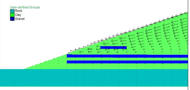
To better explain the effect on the deformation pattern of the location of the lenses, 2 configurations (namely #39 and #49) have been selected as examples and are introduced here to illustrate this localization effect. Both configurations have 20 stochastically-generated gravel lenses but the lenses distribution and their length is different. The displacement along the x direction and the displacement vectors are illustrated in the following figures.
In Fig. 6 the gravel lenses (in blue) are mainly distributed in the center of the slope and most of them outcrop at the face of the slope. Consequently, the deformations in the x direction are quite low, with a maximum of 0.6 m displacement, and concentrated at the top of the slope, where less lenses are present. It is also possible to appreciate in Fig. 7 the decrease of the vectors length every time a gravel lens is intercepted from the top to the bottom.
On the other side, in Fig. 8, the gravel layers are smaller and they have fewer outcrops. The displacements are therefore higher and their pattern induce a different deformation along the surface. The comparison between Fig. 7 and Fig.
24
9 highlights that the clustering of more resistant layers is less effective than a more even distribution. However, the presence of two layers at the foot of the slope is sufficient to have the slip surface moved upslope
Fig. 6: x displacement contours for soil configuration #39 with 20 gravel lenses
25
Fig. 8: x displacement contours for soil configuration #49 with 20 gravel lenses
26
Fig. 10: vectors of displacement for soil configuration #49 with 20 gravel lenses at the foot of the slope
Compared to the zero-slope, one configuration displays a decrease of 60% of the maximum deformation in x direction, while for the other the reduction reaches almost 90%.
This simple example application shows clearly how a small variation in the stratigraphic profile of natural soils may affect the deformation behavior of a slope. This result could be useful in designing road embankments in developing countries for example. In areas where high resistance soils are not available or too costly to get in large amounts the use of small layers of gravel could highly improve the stability of the whole structure even though their position in the embankment could be not that precise. In a way, for some applications gravel layers in slope may be used as reinforcement instead of geotextiles.
3.1.2 Spatial uncertainty
Further analyses that may be done on the whole dataset of configurations in order to determine the most significant location for site investigation. In fact analyzing the mean value and most importantly the standard deviation of deformations in the same locations it is possible to see where a new borehole might reduce the most the uncertainty in the numerical models.
To do so a tridimensional matrix was created in MatLab stacking all soil configuration. Then point wise mean and standard deviation where calculated along the third dimension. Grabbing from FLAC the x,y coordinates of the
27
centroids of the mesh elements it is possible to create a .txt file which may be read easily by MatLab. A dataset with the coordinates of the centroids of each zone and the values of mean and standard deviation for each cell is assembled. For the visualization of results ARC-Map 10.1 commercial software was chosen. Through the “import X,Y” data tool each record of the dataset is converted in a point feature. The results of this procedure are illustrated in Fig. 11 and Fig. 12.
Fig. 11: mean value of x displacement for the 250 soil configurations
Fig. 12: standard deviation of x displacement for the 250 soil configurations
Even in this simple example, an evident pattern for mean values and standard deviation of results appears, which indicate that the best location for a new borehole is at the first third of the slope length starting from the top.
This tool could be extremely useful for the study of landslides, in order to select the points were uncertainty would be reduced most effectively in a new investigation campaign.
28
3.2 3D - Simple slope with horizontal layering
A similar geometry as the previous example was applied in a 3D model (Fig. 13). 3D models may be used when the effect of slopes with complex geometry may affect significantly the deformation pattern.
However, in this example we just analyze the displacement in a simple geometry but with different soil parameters of the matrix.
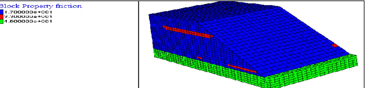
Fig. 13: geometry of the 3D example. Highlighted the friction parameter for soil configuration #22 with 15 gravel lenses – internal lenses are not visible
This was done to investigate the narrowing of the PDFs which was seen in the 2D example, with decreasing number of more resistant layers. In this case a different balance of strength parameters between matrix and layers was used in order to better analyze the interaction between soil types.
Four different couples of soil parameters for the matrix were tested (Tab. 1) with Mohr-Coulomb failure criterion keeping constant the parameters of the layers (33° friction angle and null cohesion).
Tab. 1: sets of soil parameters used for the 3D test
Friction angle [°] Cohesion [kPa]
Test 1 19 8
Test 2 18 8
Test 3 17 8
Test 4 16 8
A number of 250 soil configurations were calculated, 50 for respectively 5, 10, 15, 20, 25 gravel lenses. The geometry of the mesh is quite simple and composed by
29
18774 brick and wedge elements. 12600 are of matrix material subject to the stochastic generation of soil layers, the rest is bedrock and does not change. The computational time for each soil configuration is approximately 4 minutes on a 3.10 GHz processor with 4 GB of RAM, therefore for 250 runs the calculation time is nearly 16 hours.
In Fig. 14 and Fig. 15 as an example two soil configurations with 15 gravel lenses and with the same soil parameters are confronted. The maximum displacements are almost one the half of the other. Moreover the deformation pattern differs significantly in function of only the relative position of the lenses.
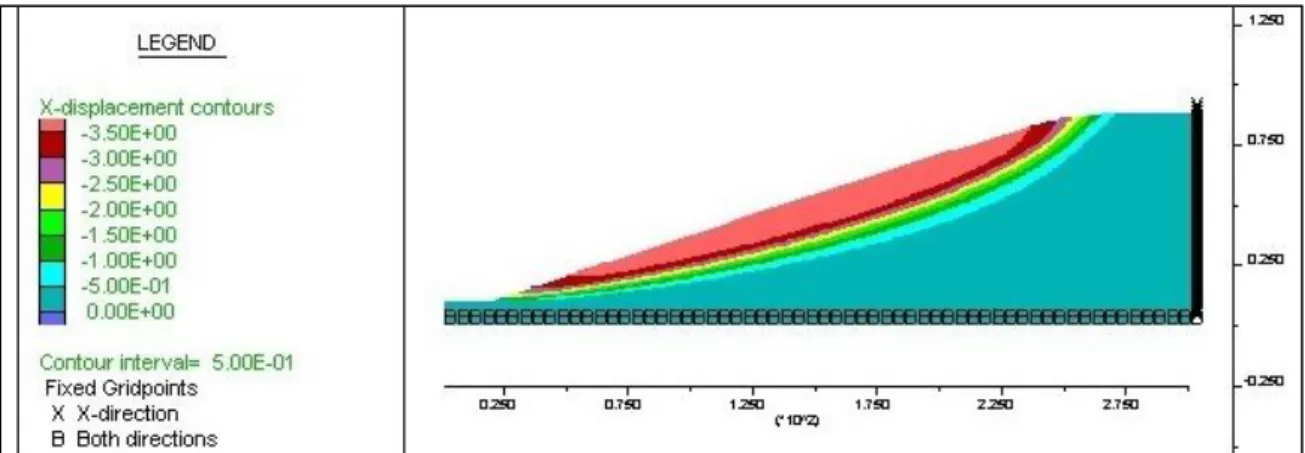
Fig. 14: X displacement contours for soil configuration #22 with 15 gravel lenses and 17° matrix friction angle and 8 kPa cohesion
Fig. 15: X displacement contours for soil configuration #7 with 15 gravel lenses and 17° matrix friction angle and 8 kPa cohesion
In Fig. 16, Fig. 17 and Fig. 18 and the distribution of the maximum deformations for respectively angle of friction of the matrix 19°, 18° and 17° are presented: the clustering of solution for lower numbers of layers is evident and it increases lowering the angle of friction. However, when the angle of friction of the matrix is 16° the deformations increase dramatically (Fig. 18). In this case the PDFs are narrower the bigger is the number of gravel layers, because their presence
30
guarantees a minimum of support which is independent from the positioning of the layers.
Fig. 16: maximum deformations for the 3D slope with matrix parameters of 8 kPa of cohesion and 19° of friction—the bell curves represent the PDF of each set scaled on the area
Fig. 17: maximum deformations for the 3D slope with matrix parameters of 8 kPa of cohesion and 18° of friction—the bell curves represent the PDF of each set scaled on the area
31
Fig. 18: maximum deformations for the 3D slope with matrix parameters of 8 kPa of cohesion and 17° of friction—the bell curves represent the PDF of each set scaled on the area
Fig. 19: maximum deformations for the 3D slope with matrix parameters of 8 kPa of cohesion and 16° of friction—the bell curves represent the PDF of each set scaled on the area
32
Through the analysis of the mean displacement for every angle of friction of the matrix the effect on the standard deviation of the PDF for lower number of layers is less evident (Fig. 20, Fig. 21 and Fig. 22). However, as for the maximum displacements, for 16° of friction angle the standard deviation of the PDF increases significantly for low numbers of gravel layers (Fig. 23). Thus the variation of the size and the positioning of the more resistant strata influence greatly the kinematic of the slope. Within a distribution of 50 soil configurations of 5 layers the mean value of horizontal displacement may vary between 0.2 m to almost 1.2 m.
Fig. 20 mean deformations for the 3D slope with matrix parameters of 8 kPa of cohesion and 19° of friction—the bell curves represent the PDF of each set scaled on the area
33
Fig. 21: mean deformations for the 3D slope with matrix parameters of 8 kPa of cohesion and 18° of friction—the bell curves represent the PDF of each set scaled on the area
Fig. 22: mean deformations for the 3D slope with matrix parameters of 8 kPa of cohesion and 17° of friction—the bell curves represent the PDF of each set scaled on the area
34
Fig. 23: mean deformations for the 3D slope with matrix parameters of 8 kPa of cohesion and 16° of friction—the bell curves represent the PDF of each set scaled on the area
35
4 The Mortisa landslide case study
4.1 Study areaThe Mortisa landslide is located on the west slope of the Cortina d’Ampezzo valley (Veneto, Italy), part of the Dolomites UNESCO World Heritage list.
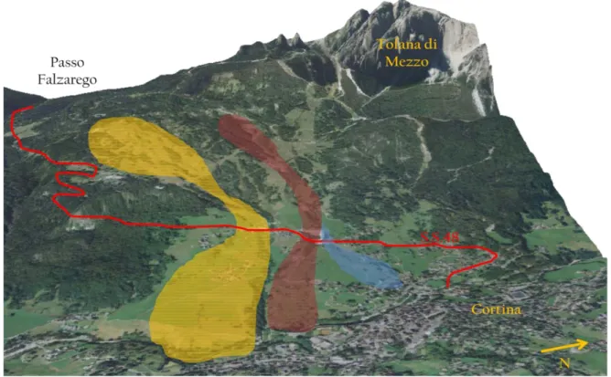
The landslide unit is composed by three slow moving mudslides (Fig. 24) with the typical "hourglass" morphology (Glastonbury & Fell 2008) namely:
• Sector 1: the most southern landslide, which moves under the Mortisa village, in yellow in Fig. 24.
• Sector 2: the central landslide, in red in Fig. 24, which is the most active. • Sector 3: a smaller mudslide, that originates from the track zone of Sector 2 directing to the village of Grignes.
The whole affected area is 3500 m long, stretching from 1750 to 1300 m a.s.l. (Fig. 24). The landscape is characterized by the presence of the magnificent Tofane dolomitic Group that reaches 3244 m a.s.l.
36
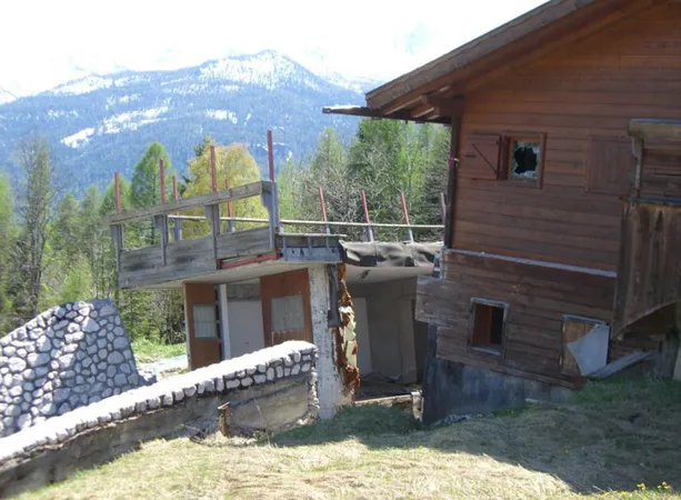
For the significant geo-lithological differences and the variations of altitude and exposure, the area shows a wide variety of physical and geographical environments. Upstream, the landscape is dominated by the vertical walls of the Tofane and by debris deposits accumulated at the foot of dolomitic limestone reliefs. Further downstream alternating meadows and wooded slopes are founded along with the ski slopes and the ski lifts that are the primary anthropogenic element located above the National Road, (SS 48). Below a fairly dense urbanized area follows, where the settlements of Mortisa, Lacedel and Grignes are found. The movement interferes with the national road and secondary road network and during the years it has damaged several buildings (Fig. 25). Due to these landslide risk conditions, the movements have been investigated since 1998.
Fig. 25: a building along Sector 2 completely destroyed by the landslide moments
4.2 Geology
They study area is characterize by the presence of the Dolomites, mountain ridges which have their upper part of dolomite rocks. Organic reefs formed on deposits
37
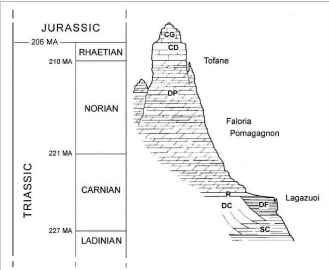
of volcanic, carbonaceous or calcareous origin in the Triassic sea which at that time covered the area. These deposits are layered weak rocks masses, with marl or limestone strata alternating with thin clay shale and claystone layers forming packs up to 1 m in thickness (Soldati et al. 2004). On top the reefs recrystallized into Dolomite rocks and now their thickness reaches some hundreds of meters (Fig. 26).
Fig. 26: Stratigraphic sequence outcropping in the Cortina d’Ampezzo, valley (modified after Bosellini 1996). CG: Grey Limestones; CD: Dachstein Limestones; DP: Dolomia Principale; R: Travenanzes Fm.; DC: Dolomia Cassiana; DF: Durrenstein Fm.; SC: San Cassiano Fm.
The rock types outcropping in Cortina d’Ampezzo (Fig. 27) developed in a period embracing the Middle Triassic to the Jurassic and can be distinguished in:
Dolomites and limestones from Middle Triassic to Middle Jurassic (Dolomia Cassiana; Durrenstein Formation; Dolomia Principale; Dachstein Limestones; Grey Limestones).
38
Calcarenites alternating with marls and clay shales from the Middle-Upper Triassic (S. Cassiano Formation and Travenanzes Formation) cropping out at the foot of the dolomite cliffs, forming the upper part of the valley flanks. The Raibl Formation outcrops between the Dolomia Principale and Dolomia Cassiana.
Fig. 27: geological map of the area surrounding Cortina d’Ampezzo (Panizza et al. 1996). 1: San Cassiano Formation, Durrenstein Formation and Dolomia Cassiana; 2: Travenanzes Formation and Dolomia Principale; 3:other formations; 4:thrust; 5:fault
4.3 Stratigraphy
The study area has been investigated throughout the years in order to comprehend the causes and the evolution of the movements of the landslide.
4.3.1 1989 investigations
The investigation campaigns of 1989 of Genio Civile (Civil Engineering Board) have focused on the stretch of Sector 2 below the national road. The location of
39
the boreholes is indicated in Fig. 28. In this paragraph we briefly illustrate the most significant elements of the cores.
S1-89 is a 20 m deep borehole located at 1188 m a.s.l. a layer of sandy gravel was found with evidence of water circulation between 10 and 13 m from the ground level; another layer of debris was found between the portion 18 and 16.70 meters. The rest of the material consists of silty-clay.
The stratigraphy of the S2-89 (1175 m a.s.l.,) consists of silty-clay in the first 6 feet of gravel in the following four.
S3-89 is located at 1225 m a.s.l.. Alternations of silty-clays and shallow layers of gravel were found along the whole core that is 40 m long.
Stratigraphically the S4-89 survey (1187 m a.s.l. 35 m) comes as a single layer of silty-clay with different consistency: soft on the surface, especially in the first 6 meters from the surface, and compact in the deeper layers. Locally layers with greater presence of gravel clasts in the clay matrix were found.
S5bis-89 is located along the Nation Road at 1302 m a.s.l. and consists predominantly of compact silty-clay, with a level of dolomitic pebbles of 3 meters located between 44 and 47 m from the surface and another one of 2 m between 13 and 15 m.
The stratigraphy of S7-89 consists of silty-clay, more plastic in the first ten meters and then compact; locally layers with clastic inclusions are present.
4.3.2 1991 investigations
In 1991 two other boreholes were performed in the area by researchers of the CNR-IRPI (National Research Council – Research Institute for Geo-Hydrological Protection) in order to install two inclinometers. The drilling technique was continuous core drilling therefore it was possible to examine the cores.
Survey S1-91, located in the area above the confluence of the 2 main channels of the slope at 1240 m a.s.l., reached the bedrock, the San Cassiano Formation, at 61 meters below the surface. The soil consists of plastic clays with inclusions of various sizes; between 44 and 19 meters, and between 55 and 61 there are two layers of gravel.
S2-91 borehole (1246 m a.s.l.) is 21 m long and does not reach bedrock; it consists of compact silty-clay with local inclusions of gravel.
40
Fig. 28: investigation boreholes for the 1989 and 1991 campaigns.
4.3.3 2009 investigations
During the investigation campaign of 2009 three boreholes were drilled. The perforation activity began on May 4, 2009 and ended July 14.
The choice of the locations for the new boreholes was made in order to analyze the behavior of the external portion of the landslide, where lower rate of activity wasto be expected. This was linked to the fact that the boreholes were to be equipped with inclinometric tubes and it was probable for the instrumentation to last longer if it was placed in a zone of the landslide where little and slower movements were likely (Fig. 29).
41
Fig. 29: geomorphological map of the Mortisa area (extracted by Pasuto et al. 2005). In red are indicated what were supposed as active mudslide, in orange dormant mudslide.
Borehole S1 is located in the village of Mortisa at 1,247 m a.s.l. on Sector 1; the localization of the hole was linked to the intention to determine through inclinometric surveys wether that mudslide was actually dormant, as indicated by the Geomorphologic map of the surrounding of Cortina d'Ampezzo (Pasuto et al. 2005). The survey reached the bedrock, represented by S. Cassiano Formation, at a depth of about 60 m, in accordance with the findings of previous surveys conducted in the area. The landslide material is mainly silty-clay with dolomitic inclusions predominantly angular cobbles. The presence in the cores of 4 levels of gravel 50 cm thick has been recorded at 7, 9, 21 and 37 m, moreover two levels of some thicker than a 1 m are indicated at 44 and 46 m. Several samples were taken for laboratory testing, in particular, an undisturbed sample was extracted at depths between 28.00 and 28.50 meters deep and three samples were collected for radiocarbon dating.
The second survey was performed near the settlement of Lacedel, between Sector 1 and 2 at an altitude of 1312 m a.s.l. In this case bedrock has been reached at a depth of about 40 m (the material is still S. Cassiano Formation). The materials composing the cores appear similar to those found in S1 even though gravel layers are thicker. Among those layers the most thick is the one of five meters between 22 and 27 m; however other 7 layers more than a meter thick are present.
S2
S1 S3
42
Borehole S3 was placed near the village of Grignes at an altitude 1253 m a.s.l. The drilling did not reach the bedrock and was stopped at 66 m. The stratigraphy differs fairly from what was found in S1 and S2. Several levels of angular dolomitic gravel of considerable thickness are present in the first 30 m, then gravel becomes predominant. These levels could be attributed to debris flow deposits.
4.4 Geomorphological evolution of the Mortisa landslide
The geomorphological evolution of the valley of Cortina d’Ampezzo has been broadly studied.
Geomorphological features are obviously related to the underlying stratigraphic geological sequence. The succession of rigid and more plastic bodies influenced deeply the structure of the slopes (Bosellini 1996) which were strongly moulded by the processes triggered by the final withdrawal of stadial valley glaciers of the Lateglacial (Borgatti & Soldati 2010) between some 14,000 and 11,000 cal BP (van Husen 1997). In this period a progressive rise in temperature has been ascertained followed by an increase of precipitations. An increase of landslide activitiy has been correlated with this climate change (Soldati et al. 2004) through the analysis of organic samples extracted in landslide bodies.
As part of the Mortisa landslide investigation 6 wooden samples were extracted from the cores to be analyzed through radiocarbon dating. These samples integrated the database of the area that consisted in 3 entries obtained in 1991 (Tab.2) (Soldati et al. 2004; Borgatti & Soldati 2010).
43
Tab. 2: radiocarbon dating
Borehole m a.s.l. borehole Depth sample MATERIAL Conventional age Type of soil matrix S1 1247 - 12 (wood):
acid/alkali/acid 4290 +/- 40 BP Silty clay
S1 1247 - 44 (wood): acid/alkali/acid 8930 +/- 40 BP contact gravel/silty clay S1 1247 - 52.9 (wood):
acid/alkali/acid 9700 +/- 60 BP Silty clay
S2 1312 - 27.5 (wood): acid/alkali/acid 3930 +/- 70 BP contact gravel/silty clay S3 1253 - 61.5 (wood): acid/alkali/acid 8410 +/- 180 BP gravel S3 1253 - 27.2 (wood):
acid/alkali/acid 6740 +/- 60 BP Silty clay
S1-91 1238 - 43.3 wood 10035+/- 110 BP
contact gravel/silty
clay
S2-91 1246 - 22.2 wood 9270+/- 105 BP Silty clay
44
Fig. 30: location of organic sample extraction for radiocarbon dating
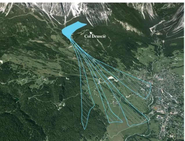
Chronological data interpretation suggest that mudflows affecting the San Cassiano Formation, which is composed by calcarenites, marls and clay shales outcropping at the foot of the dolomite cliffs (Neri et al., 2007) were the first type of slope instability event . Then, a massive rock slide detached from the dolomite units forming the so-called Col Drusciè landslide (marked as CD in Fig. 30). The presence of Col Drusciè influenced greatly the evolution of the landscape. To analyse this dynamic the hydraulic catchment of the slope of Mortisa was identified using Hydrology tools of ArcMap 10.1 on the basis on a 1x1 m LiDAR Digital Terrain Model (DTM). The basin area is 7.4 km2 and is represented in Fig. 31.
From Fig. 31 it is clear that Col Drusciè created an upper basin between the dolomitic flanks of the Tofane Group and the Boite valley. The water which was flowing directly in the Boite torrent it is now gathering into the new basin directed firstly southwards and then merging in the other east-west directed channel (Fig. 32).
45
Fig. 31: watershed of the Mortisa slope
Fig. 32: blue lines for the Mortisa catchment
Col Drusciè
N
Col Drusciè
46
In addition, coarse sediments originating from the Tofane group and from the scarp of the rockslide accumulated in the little basin to be then available for transport. Debris flows triggered by heavy precipitations moved the gravel material along the slope, probably following the old channels, eventually changing their former tracks and runout back and forth across the alluvial fan because of diversion phenomena. This assumption is also coherent with stratigraphic data which indicate a larger amount of gravel lenses with greater thickness in the northern cores.
Fig. 33: schematic dynamic of postglacial debris flow in the Mortisa area
Concurrently a series of silty-clay mudflows, originated from the weathering of the San Cassiano formation on the southern part of the slope, covered the gravel layers creating the alternation of the stratigraphy with time. The present Mortisa landslide body is therefore formed by interdigitated layers of silty-clay and gravel which originated from the alternation of mud and debris flows affecting the slope during the Holocene.
47
To endorse this hypothesis other piece of evidence concur. A series of permeability test were performed by the Civil Engineering Board by means of sub-horizontal drainage pipes that were installed in the lower track of the central slide. From the data it was possible to appreciate the scattering of the gravel lenses. The most interesting element was that significant different response was measured in pipes that were located less than 20 meters apart. This confirms the almost random distribution of the lenses of gravel. Moreover the highly permeable gravel lenses seems to be in contact with the fissured dolomitic rocks on top of the slope and the aquifer hosted in the lenses are confined in the clay matrix in the medium to lower part of the landslide body. In fact, during intense rainfall events, in the piezometers located along the slope, variations of more than 10 m for the water table are recorded.
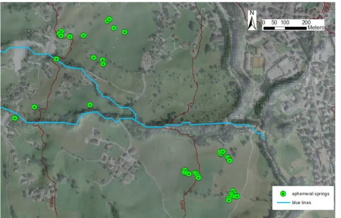
Lastly, a survey to locate with GNSS ephemeral springs and pools was performed (Tromboni 2013). The survey was executed during snowmelt, after a conspicuous rise of temperature (+10°) which following an intense snow precipitation. These springs represents areas with greater hydraulic conductivity therefore are probably related to the presence of gravel layers. In Fig. 34 it is possible to appreciate the scattering of data in the study area. Unfortunately, it was not possible to inspect the area along the ski slopes located between 1350 and 1550 m a.s.l. because maintenance work were conducted and access was forbidden.
48
Fig. 34: ephemeral springs located in the Mortisa slope
A cluster of springs and pools was found south of Col Drusciè (Fig. 35). This is coherent with our geomorphological hypothesis since we suppose that the greater amount of coarse sediment would have come from the basin located between Col Drusciè and the Tofane group.
In the lower part of the slope many springs outcrop Fig. 24. They are located mostly on Sector 1, in the Mortisa fan, and in the area where Sector 2 and Sector 3 are in contact. The large presence of springs in the latter area may be linked to the significant movements occurring in the zone which may increase hydraulic conductivity also by deforming and disaggregating the soil. Moreover in the area a larger amount of gravel is expected since debris flow where more likely to run in this direction.
On the other side the great number of springs and pools marked at the foot of Sector 1 may be linked to the outcrop of the slip surface of the mudslide for the upper group and to the contact between the bedrock and quaternary bodies for the lower group.
49
Fig. 35: ephemeral springs located in the upper part of the Mortisa slope
Fig. 36: ephemeral springs located in the lower part of the Mortisa slope
50 4.5 Monitoring network
4.5.1 GNSS benchmarks
The GNSS (Global Navigation Satellite System) control network for the monitoring of surface deformation of the landslide Mortisa was materialized in July 2008. The local network control consists of one benchmark located in an area considered stable outside the landslide in the village of Ronco, North of Lacedel. The choice of the site was made according to various requirements such as: the accessibility, the possibility of having a protected location for the instrumentation, the lack of obstacles for the visibility of the satellites, a sufficient distance from sources of noise to the signal (high voltage cables, repeaters, etc.), minimum distances between points and dimensions similar to those of the area to be monitored.
In the landslide area 30 benchmarks were materialized, some of which were located outside the most active part in order to verify the actual extension of the mudslides. The points were materialized with topographic nails fixed in the asphalt (unfortunately it was not possible to have many nails on the national road because maintenance works were scheduled) and with forced centering devices in order to avoid positioning errors.
Two different survey techniques were used. For points materialized with the forced centering devices a relative positioning of the static type was chosen with dwell time of 10 minutes, sampling every 2 sec (300 measures to point) and angle of cut-off of the antenna equal to 15 °. The use of this technique is linked to lack of radio signal, given the distance between the target point and some control points. The position of the remaining pillars was determined with a fast static rapid real-time survey with sampling time of 1 second, acquisition time of 2 minutes and a cut-off angle of the antenna of 15°.
51
Fig. 37: GNSS planar displacements recorded between July 2008 and April 2012
From the analysis of the data (Fig. 37) it can be seen that the entire slope is in motion but with different rate of displacements. In fact there are areas of displaying largert activity, in which the displacements are of the order of meters/year and others in which the deformations are centimetric.
Sector 1 is globally the least active even though benchmark 7, installed on a check dam, in 4 years has moved more than 3.3 meters. As the check dam does not show structural damage the depth and extent of the landslide in that section is made clear. Sector 2 shows pronounced deformations, especially in the benchmarks located below the national road where the displacements velocities exceed 1 meter per year. It is most likely that the earth works that were needed in order to guarantee a bigger parking space for the access to the ski slopes caused an overload which aggravated the instability.
Finally, also in Sector 3 there are benchmarks which show large planar deformation; some of these, especially in the upper part (10 and 11), showed significant vertical deformations in the order of cm/year too. To increase the number of available data and have a better understanding of the dynamics of the
52
crown of Sector 3 new benchmarks were installed (the last, named 32, in April 2012) on the side of the national road which, however, were lost as a result of maintenance work performed in the area.
Through the analysis of the GNSS data it was possible to identify Sector 2 as the most active, therefore in the following chapters we will focus on this mudslide, avoiding to illustrate monitoring results for Sector 1 and Sector 3 for clarity.
4.5.2 Inclinometers on Sector 2
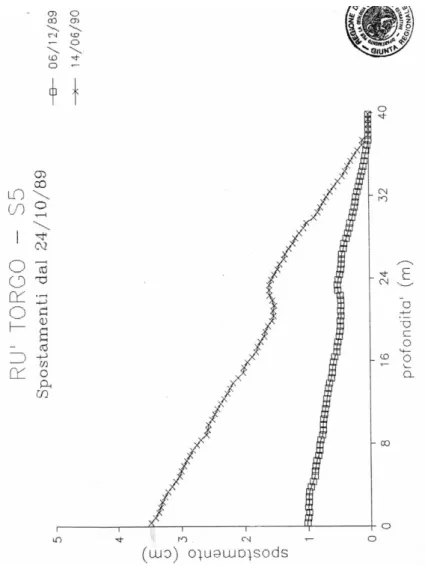
Sector 2 is the most investigated since it shows greater deformations and its movements damage the main road network of the area. For these reasons, in the 1989 campaign a borehole of 51 m equipped with an inclinometric tube was placed near the National Road. From Fig. 38 it is possible to hypothesize the presence of a slip surface at 38 m below the ground surface.
.
53
Another inclinometric tube was installed in S2_91 borehole, located in the center of the lower Sector 2 track (Fig. 28). The inclinometer data show a clear deformation at 10 m below the ground surface. The deformation indicated in Fig. 39 developed in 14 days, then the tube broke and it was not possible to carry out other measurements.