Toward a Magnitude Scale for Low Frequency Seismicity The LP energy for Campi Flegrei caldera

(1)

Alma Mater Studiorum – Università di Bologna

DI RICERCA IN

DOTTORATO

GEOFISICA

Ciclo XXV

Settore Concorsuale di afferenza: 04/A4 Settore Scientifico disciplinare: GEO/10

TITOLO TESI

TOWARD A MAGNITUDE SCALE FOR LOW

FREQUENCY SEISMICITY

The LP energy for Campi Flegrei caldera

Presentata da: IRENE BORGNA

Coordinatore Dottorato Relatore

Prof. Michele Dragoni Dr.ssa Francesca Bianco

(2)

(3)

3

1. Abstract

The energy released during a seismic crisis in volcanic areas is strictly related to the physical processes in the volcanic structure and could be a very important parameter to study in activities dealing with eruption forecasting. In particular Long Period seismicity, that seems to be related to the oscillation of a fluid filled crack (Chouet , 1996, Chouet, 2003, McNutt, 2005), can precedes or accompanies an eruption; these seismic signals may be used to assess the eruptive state of a volcano or its eruptive potential.

The present doctoral thesis is focused on the study of the Long Period seismicity recorded in the Campi Flegrei volcano (Campania, Italy) during the October 2006 crisis.

Campi Flegrei Caldera is an active caldera (situated in a densely populated area in the North of Naples); the combination of an active magmatic system and a dense populated area make the Campi Flegrei a critical volcano.

The source dynamic of LP seismicity is thought to be very different from the other kind of seismicity ( Tectonic or Volcano Tectonic): it’s characterized by a time sustained source and a low content in frequency. This features implies that the duration–magnitude, that is commonly used for Volcano Tectonic events and sometimes for LPs as well, is unadapted for LP (and VLP) magnitude evaluation. The main goal of the research work performed in the framework of the doctoral studies was to develop a method for the determination of the magnitude, for the LP seismicity; we based this method on the comparison of the energy of VT event and LP event, linking the energy to the moment magnitude for the VT. So the magnitude of the LP event would be the moment magnitude of a VT event with the same energy of the LP. We applied this method to the LP data-set recorded at Campi Flegrei caldera in 2006, to an LP data-set of Colima volcano recorded during an experiment performed in 2005 – 2006 and for an event recorded at Etna volcano.

Experimenting this method to lots of waveforms recorded at different volcanoes we tested its easy applicability and consequently its usefulness in the routinely and in the quasi-real time work of a volcanological observatory.

(6)

6

2. Introduction

Volcanoes are geologic manifestations of highly dynamic physical and chemical processes in the interior of the Earth.

Volcanic eruptions and their impact on human society are one of the most severe natural hazards.

Often, before an eruption, a series of phenomena indicative of an abnormal state of the volcano occurs; this phenomena are defined precursors. They include the increasing in the frequency and/or intensity of the earthquakes located below the volcano apparatus, the presence of volcanic tremor, the uplift of the soil, the opening of fractures, the increasing in fumarolic activity and the variation in its temperatures and composition, the compositional variations of the fluids involved…

Their presence, duration and time interval before the eruption depends on factors that currently remain largely unknown. So the study of their temporal evolution may be very helpful in a monitoring context. Precursory observation often coincided with the starting of an eruption in open-conduit volcanoes, but the situation is more complicated in the case of quiescent volcanoes like Campi Flegrei caldera.

Volcano seismology aims to understand the nature and dynamics of magmatic systems, and to determine the extent and evolution of source regions of magmatic energy which are important for the understanding of the volcanic behavior. The energy released during a seismic crisis is strictly related to the physical processes in the volcanic structure and could be very important in eruption forecasting.

The study of the Low Frequency seismicity is relative new and therefore the knowledge about both the physical mechanisms responsible for such signals, and their propagative features it is constantly updated.

In particular, Long Period seismicity seems to be correlated with the resonance of a fluid filled crack (magmatic or hydrothermal fluid) (Chouet , 1996; Chouet, 2003, McNutt, 2005), it can precedes or accompanies an eruption hence these seismic signals may so be used to assess the eruptive state of a volcano or its eruptive potential. For example, swarms of small and shallow LP events can be the only precursor of an important phreatic activity (Barberi, et al., 1992).

The seismic monitoring of the active volcanoes, such as Campi Flegrei, is necessary to put in evidence possible precursors of an imminent eruption. Unfortunately, there is no clear relation between the energy of the precursory seismicity signals and the strength of the subsequent eruption.

(7)

7

The present doctoral thesis is focused on the study of the Long Period seismicity recorded in the volcano of Campi Flegrei (Campania, Italy) in the October 2006.

Campi Flegrei Caldera is an active caldera (situated in a densely populated area in the North of Naples), which last eruption occurred on 1538 affecting the Monte Nuovo eruptive center (Di Vito, et al., 1999). The combination of an active magmatic system and a dense populated area make the Campi Flegrei a critical volcano, and the comprehension of the volcanic state is important to protect the population.

The source dynamic of the Long Period seismicity is thought to be very different form the other kind of seismicity: LP and VLP (Very Long Period) events are characterized by the time persistency of the source, the peak of the spectrum at low frequency (less than 5 Hz for LPs and much less for VLPs) and the absence of high-frequency components in the spectrum of their seismic radiation. One of the practical consequences of the lack of high-frequency coda is that the duration–magnitude, that is commonly used for Volcano Tectonic events and sometimes for LPs as well, cannot be used for LP (and VLP) magnitude evaluation since it could lead to confusing results. The magnitude concept comes from the relationship between the waveform amplitude of a seismic event and its energy (taking into account the path attenuation). The definition of magnitude was then firstly proposed by Richter, measuring the amplitude of an event recorded at a well-known instrument. So the seismogram can be transformed into an equivalent Wood Anderson record using the empirical curve that describes the attenuation of the maximum amplitude with the source-station distance, taking a zero magnitude reference event.

Differently from a VT event, an LP characterized by a long (source) duration and a low maximum amplitude can have the same energy as another LP event with a greater maximum amplitude and a shorter duration, so the maximum amplitude alone is not sufficient to determine the magnitude of a Long Period event.

In fact, the spectral content of the VT event, with a source-duration shorter than that of an LP event, is much broader than that of the LP event, it makes the coda of a VT reach in high frequency energy making it longer than that of the LP event.

Consequently we needed a different parameter to evaluate the energy and then the magnitude of LP events.

After its definition (Kanamori, 1977), the moment-magnitude scale came into common use for the physical definition of a tectonic earthquake strength, since, first of all, it does not saturate for large earthquakes and it is based on the physical properties of the source. It is based on the calculation of the seismic spectrum assuming a double-couple source model and a far-field

(8)

8

radiation and measuring the level of the flat portion of the source spectrum (log-log plot).

Even if the moment-tensor inversion would produce more accurate results (e.g. Aster, et al., 2008 and Auger, et al., 2006) its application in quasi-real time could be more complicated.

We consequently decided to base the developed algorithm for the evaluation of the LP magnitude, on the comparison with the energy of VT event and LP event, linking the energy to the moment magnitude for a VT.

To reach this scope we studied the LP seismicity recorded in the 2006 October at Campi Flegrei Caldera, we developed the new algorithm for the LP magnitude estimation and we applied that method to this seismicity and also to the LP seismicity recently recorded at Colima volcano (Mexico) and Etna volcano (Sicily, south of Italy).

(9)

9

3. Volcanic seismicity – source dynamic and

seismic signature

To have a clear idea of the link between the fluids transport (and therefore the volcanic activity) and the seismicity , it can be useful to classify the volcanic seismicity according to the waveform features and consequently to the physics of the source processes. A magma intrusion or oscillation perturbs the volcano edifice and leads to different kinds of signals. The large variety of seismic signals observed in volcanoes is thus the representation of the structural heterogeneity of the volcanic edifices, and can be classified into two families linked to two different sources: one originates in the rock (Volcano-Tectonic events) and the other originates in the fluid, of magmatic or hydrothermal component (Long-Period, Very Long Period, Tremor and

Hybrids).

The first kind of events is associated with the shear failure in the volcanic edifice where the magmatic processes provide the source of the strain energy that leads to rock failure. These earthquakes are called Volcano-Tectonic (VT), to discern them from the ‘pure’ tectonics events although they’re practically indistinguishable. So it is possible to discern the P and S waves arrivals and the characteristic frequency can reach value much greater than 5 Hz (Figure 1). The only difference from the ‘pure’ tectonic seismicity is the frequent occurrence of swarms of VT events, which do not follow the usual main-after-shock distribution (Wassermann, 2011). They involves purely elastic processes in the brittle rock and are often located around the conduit and magma reservoir. The VT seismicity is often the first sign of a renewed activity. The rising magma acts as an additional stress source, that superimposed to a regional stress field, leads to tensile faulting when magma is breaking the rock, or to earthquakes on preexisting faults as a reaction to additional stress.

(10)

10

Figure 1 VT event recorded at Mt. Merapi (Indonesia). Arrivals of P and S waves clearly distinguishable. The colour coding represents normalized amplitude spectral (Wassermann,

2011).

The other kind of volcano seismicity, involving processes originating by the dynamic of the fluid, inside structures such as crack, pipes or fluid filled conduits, includes Long Period (LP) events, Very Long Period (VLP) and

Tremor. The fluid component can have magmatic or geothermal origin and

the gas content can vary greatly from volcano to volcano, accordingly with the depth of the source and the fugacity of the gas itself.

LP events differ from the tectonic earthquakes in their signature and spectral characteristic. There is no clear arrival for P and S waves and its characteristic frequency varies in fact from 0.5 Hz to 5 Hz (lower than the VT’s) (Chouet , 1996) (Figure 2, Figure 3).

The VLP characteristic frequencies are lower than 0.5 Hz, while tremor have the same frequency band of LP but it differs from the latters about the duration: tremor is characterized by a signal of sustained amplitude lasting from minute to months or longer (Figure 4). This suggests that LP and tremor may have the same source process differing only in duration.

In the study of the dynamics of the whole volcanic structure, LP, VT and tremor are intimately tied together.

(11)

11

Figure 2 LP event recorded at Mt. Merapi. The dominant frequency is about 1 Hz (Wassermann, 2011).

Figure 3 Example of LP event recorded at two different stations at Redoubt volcano (Alaska) (Wassermann, 2011). The spindle shape waveform is also known as ‘tornillo’.

(12)

12

Figure 4 Tremor signal recorded at Mt. Semeru (Indonesia) (Wassermann, 2011).

Moreover, there is another kind of volcanic earthquakes, named Hybrids, that represents the transition between the two families described above, with signal and spectral characteristics of both intermediate between the LP and VT events. The hybrid events have an onset more pronounced than that of the LP, but an harmonic coda similar to the former . They are thought to involve shear faulting on a plane intersecting a fluid-filled crack, so they have both volumetric and shear component, and they can additionally reflect possible path effects (Wassermann, 2011).

This events are also related to a very shallow activity that may be associated with a growing dome (Miller, et al., 1998).

(13)

13

Figure 5 Hybrid event Redoubt volcano (Alaska) (Wassermann, 2011).

3.1 Long Period seismicity

In volumetric sources, gas, liquid and solid are dynamically coupled. The elastic radiation is the result of processes originating in the physics of the multi-phase fluid flow through cracks and conduits and the Long Period events are manifestations of such processes. The fluid (liquid or gas) may be of magmatic or geothermal origin and the gas content can vary depending on the volcano properties.

LP seismicity often occurs in the form of swarms and the similarity in the signature of individual events in some swarms strongly suggests the repetitive excitation of a stationary source in a non-destructive process.

Long Period events show no S-wave arrival but a very emergent signal onset (see, for instance, Figure 2) and, in the still rare cases in which the location of source are determined, they are often situated in the shallow part of the volcano (< 2 Km) (McNutt, 2005).

The source of the low frequency events is believed to be due to the mechanism of resonance produced by the oscillation of a fluid (magma or hydrothermal fluid) within cracks due to a perturbation of short duration (Chouet, 2003).

The LP events may be suitable to describe the volcanic and hydrothermal processes, since the properties of the resonator system may be inferred from the complex frequencies of the decaying harmonic oscillations in the tail of the seismogram.

The damped oscillations in the LP coda are described by two parameters, f and Q; f is the frequency of the dominant mode of oscillation, and the parameter Q represents the quality factor of the oscillatory system (other than the quality factor of the earth medium). The observed Q may be expressed as:

Eq. 1

(14)

14

where represents the radiation losses at the fluid-rock interface (is a function of the impedance contrast at the fluid-rock interface and of the geometry of the resonating cavity) and represents the intrinsic attenuation of the fluid vibration depending only on the fluid properties (Saccorotti, et al., 2007).

Typical frequencies observed for LP events are in the range 0.5–5 Hz (Chouet , 1996), and typical observed Q range from values near 1 to values larger than 100. In the following figure (Figure 6) waveforms recorded at different volcanoes and characterized by different Q values are represented.

Figure 6 Waveforms of LP events recorded at different volcanoes: Kusatsu-Shirane, Galeras, Kilawea and Redoubt. The signatures are characterized by different Q values: the Q values of Kilawea and Redoubt events are between 20 and 50, the Q values of Kusatsu-Shirane and galeras

are higher than 100 (Chouet, 2003).

Once spectral peaks are identified in the wavefield of a LP event, to hypothesize and to test a model for the resonator source represents the next step.

Many geometries are possible resonators (pipes, spheres, cracks…) but the one that better explains the seismic data accordingly with mass transport conditions is the crack model (Chouet , 1996).

The fluid-filled crack model was originally proposed by Aki (Aki, et al., 1977) and has been extensively studied by Chouet (Chouet, 2003 and references

(15)

15

therein) using a more formally detailed description of the coupling between fluid and solid.

This model consists in a rectangular crack with length L, width W and thickness d, filled with a fluid of density ρf, bulk modulus b and acoustic

velocity a. The crack is in a solid half space with density ρs, rigidity µ and

compressional velocity α.

The resonance is impressed by a pressure transient applied symmetrically in a small area in the center of the crack (see Figure 7).

Figure 7 Geometry of the crack model (Chouet, 2003).

The crack resonance is controlled by two parameters: the crack stiffness C and the impedance contrast Z (Eq. 2):

Eq. 2

The stiffness controls the dispersion characteristics of the wave and the resonant frequencies generated by the source. The frequency is also controlled by the impedance contrast Z, that controls the duration of the signal too. The presence of gas bubbles can reduce the acoustic velocity and thus make possible the resonance at long period, and it can also increase the signal duration (increasing the Z). The long period signal can also be generated for an increasing of the C value (increase the phase velocity of the crack wave) if the crack is characterized by a large aspect ratio L/d or large contrast b/µ.

(16)

16

Once assumed a model for the crack-source, the properties of the resonator system can be determined from the complex frequency related to Q and f (Nakano & Kumagai, 2005) of decaying harmonic oscillations in the tail of the seismogram. The complex frequency is defined as where √ , f is the frequency and g the growth rate related to the quality factor of the resonator Q because ⁄ which represents the fractional loss of elastic energy in each oscillation cycle at frequency f (Kumagai & Chouet, 1999).

A spectral method, named Sompi, was developed to quantify the spectral properties of the harmonic signals (Kumazawa, et al., 1990).

So the properties of the fluid involved in the resonator may be deduced from the spectrum of the LP seismicity, but, to better constrain the possible results, a knowledge of geological and geochemical characteristics of the area are necessary (Chouet, 2003).

(17)

17

4. Campi Flegrei Caldera

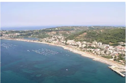
The area of Campi Flegrei (‘burning fields’ from the greek) is located 15 km west north-west of the city of Naples, is almost circular area of size 12x15 Km, inhabited by 0.5 million people.

The Campi Flegrei is a caldera with, inside, numerous volcanic structures, formed during the various eruption, subsequent to those that caused the formation of the caldera.

Figure 8 Campi Flegrei area, with the main volcano structures (Vulcani d'Italia - Uniroma3).

In Campania, the volcanic activity began around 150,000 years ago, in the Ischia island, and later in the Procida island, but in the Campi Flegrei area, the first manifestations, characterized by numerous and also violent eruptions, are probably occurred later, about 50-45000 years ago in the area of Cuma, although perforations made for the realization of geothermal wells, have shown the presence of other products arising from a previous activity. The eruption activity was concentrated in three phases separated by quiescence periods of 1000 and 3500 years (Di Vito, et al., 1999).

The most important eruptions is undoubtedly the gigantic eruption of

Campanian Ignimbrite (CI) (37-40,000 years ago) whose eruptive products,

mainly ash and pumice, spanning an area that is covering the ‘Piana Campana’ up to the Apennines, with thicknesses that reach to 100 m (Scandone &

(18)

18

Giacomelli, 1998). They are almost absent in the central part of the Piana, either due to erosion, either because they are covered by the products of the next activity of Vesuvius and Campi Flegrei themselves and by alluvial soils. The theories on the genesis of CI are numerous. According to some reconstructions (Rosi , et al., 1983) (Rosi & Sbrana, 1987), this eruption occurred along a circular fracture which coincides with the edge of the current Campi Flegrei; the rapid emission of about 80-100 km3 of magma caused the collapse of the roof of the magma chamber and the formation of the caldera depression.

According to Lirer, et al., (1987), however, the eruptive fracture included a larger area reaching the Bay of Naples, while Scandone et al. (1991) it had a NE-SW orientation and ran laterally to the Campi Flegrei. According to these authors, the origin of the Phlegrean caldera is to reconnect to a later stage than that of Ignimbrite Campana, the so-called Neapolitan Yellow Tuff eruption, whose products are widely distributed on the edge and inside the caldera (12000 years ago).

After this eruption the central part of the Campi Flegrei collapsed, forming the caldera (Lirer, et al., 1987). Although smaller than the volume of Ignimbrite Campana (20 to 50 km3 of products, covering over 350 km2), after the NYT eruption, the morphological appearance of the area changed a lot, giving the Gulf of Naples, more or less its present appearance.

According to Scandone (Scandone R., et al., 1991) after the eruption of the NYT, the lowest part of the Campi Flegrei has been submerged by the sea. The activity outside the caldera ends with this eruption, and the successive eruptions are confined within or along the edge of the caldera itself. The post-caldera activity is evidenced at the edge of the post-caldera itself by the cone of

Gauro Tuff, with an age of about 10000 years. Around 8000 years ago, a large

plinian eruption (Pomici Principali), occurs in the eastern area of Campi Flegrei. Is thought that this explosive eruption was followed by the eruption that built the island of Nisida and perhaps by another eruption on the crater rim where lately was formed the Solfatara.

Around 6000 years ago, after a period of stagnation in activity, evidenced by a paleosol, the central part of the Campi Flegrei begins to rise. In Pozzuoli, the movement of the soil is testified by a layer of marine sediments raised by about 40 m above the sea level.

Between 4500 and 3500 years ago, an intense eruptive activity returns in the Campi Flegrei (Astroni, 3700 years ago, and Monte Spina, 4000 years ago); the latest eruptions related to this phase of activity is the eruption of Senga and the Averno (Scandone & Giacomelli, 1998).

Subsequently, the soil of the Campi Flegrei, in its central part, begins to fall slowly in coincidence with a period of stagnation in the eruptive activity.

(19)

19

In Roman times, continued subsidence forced to incessant repair and rehabilitation of the road Erculea, Roman buildings along the coast are gradually reached to the sea, and, around the ninth century AD, the city of Pozzuoli is partially submerged. This phenomenon, which will be explained in more detail in the next section, is called bradyseism, and is thought to be probably related to the gradual readjustment of the soil after the release of large volumes of magma (which occurred in previous eruptions).

The last eruption in the Campi Flegrei happened in the 1538, and the volcanologists have tried to reconstruct the eruptive dynamics from the studies of the historical chronicles the detailed study of the deposits.

Around the 1502, the inhabitants of Pozzuoli noted that new stretches of beach are forming and in 1536 begins a new swarm of earthquakes, which become continuous and violent in the last week of September 1538, when the sea retired before the Tripergole village, near the Averno lake.

At one o'clock in the morning of September 29th, near the sea, a bulge comes from the cold water, probably due to the increased pressure caused by magma on the underground aquifer. Quickly this water is transformed into a cloud of steam and mud that rises in the sky, forming a characteristic mushroom-shaped column and destroying a small group of houses, after that begin to be ejected even pumice and scoria.

After this stage, follows a more properly magmatic phase, perhaps with the issue of scoria and pyroclastic flows. The last stage of the October 6th, is characterized by strombolian activity.

In a few days a mound of about 130 m is formed, and is called, with little imagination, Monte Nuovo (Vulcani d'Italia - Uniroma3).

The volcanic history of Campi Flegrei cannot be considered completed just because there have been 'only' about five hundred years after that eruption, in which there was a large urban explosion that completely ignores the possible risks too.

(20)

20

Figure 9 Crater of Monte Nuovo, (a) from (Vulcani d'Italia - Uniroma3), (b) (OV-INGV)

Figure 10 Disposition of volcanic systems in the Phlegrean caldera. The dashed lines approximate the areas of lowering, as a result of the Ignimbrite Campana eruption (the external one) and the

Tufo Giallo Napoletano eruption (the internal). (Vulcani d'Italia - Uniroma3)

(a) (b)

(21)

21

4.1 The bradyseism and seismic activity at Campi

Flegrei

One of the peculiarities of the Campi Flegrei area is the phenomenon of bradyseism (from the greek ‘slow movement of soil’), which consists of a raising of the ground, often very clear, followed by a phase of slow subsidence.

The phases of uplift are usually accompanied by seismic activity, while the phase of subsidence is aseismic (e.g. Saccorotti, et al., 2001, and references therein).

The place that, more than any other, shows this phenomenon is the Macellum (roman market better known as the Temple of Serapis, Figure 11) located near the port of Pozzuoli. The ruins of this building (which dates from the late first century AD) have been very useful for the reconstruction of bradyseism phases and in particular of changes in soil level compared to the marine’s, observing the holes produced, on the columns, from Lithodomes (mollusks living in the coastal environment in the limit of the free surface) Figure 11 (Morhange, et al., 2006).

Submersion of Pozzuoli (up to 7 m) wasn’t a unique event, but included three maximum threshold oscillations between the fifth and the fifteenth centuries A.D. The first two (400-530 A.D. and 700-900 A.D.) weren’t followed by a volcanic eruption, but the last one was culminated with the 1538 Monte Nuovo eruption (Morhange, et al., 2006).

Vertical ground deformation is common in active calderas but they are not always followed by an eruption. Generally, ground deformation is due to an inflation of magma at depth, so it reflects an evolution of magmatic system possibly ending with an eruption.

In the Campi Flegrei case, the hydrothermal fluids circulating between the surface and the magmatic chamber plays an important role.

(22)

22

Figure 11 Temple of Serapis in Pozzuoli (Vulcani d'Italia - Uniroma3).

Figure 12 Submerged Roman port in the gulf between Baia and Bacoli (Vulcani d'Italia - Uniroma3)

In the last four decades, Campi Flegrei caldera has been among the world’s most active caldera characterized by intense unrest episodes involving huge ground deformation and seismicity, but has not culminated in an eruption. The most recent high intensity bradyseismic crisis, is in the period 1982-1984 (Battaglia M. , et al., 2006, Petrazzuoli, et al., 1999, Bianchi, et al., 1987). In this period there was a noticeable uplift of 1.8 m in the area of the town of Pozzuoli, accompanied by more than 16,000 earthquakes with maximum magnitude M = 4 (these events were recorded by the first mobile digital seismic network, managed by the University of Wisconsin).

Since January 1985, began a phase of slow subsidence, interrupted by short phases of uplift in 1989, 1994, 2000 .

(23)

23

Among these episodes, the one of 2000 (July-August) is accompanied by two seismic swarms, the first of which is characterized by long-period events (LP), never recorded in the Campi Flegrei until that time.

Since August 2000, begins a new phase of subsidence until November 2004, which starts a new light uplift (4 cm) ending in October 2006.

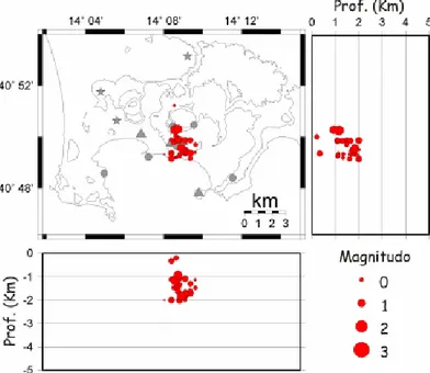
In the period between January 1st and April 14th 2006, only seven microearthquakes were recorded in the Campi Flegrei area. However, throughout the second half of 2006, there has been a strong activity, with the highest number of events since 1985. In fact, 1043 seismic events of small magnitude have been recorded, most of which located in the area of the Solfatara: 166 of these were classified as volcano-tectonic and 877 as Long Period (LP). Their localizations are shown in Figure 13:

Figure 13 Localizations of VT events, recorded between 19th and 28th October 2006, in the Campi Flegrei Caldera. (OV-INGV)

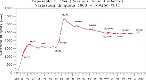
A summary of the history of ground deformation at Campi Flegrei is represented in the following figure (Figure 14).

(24)

24

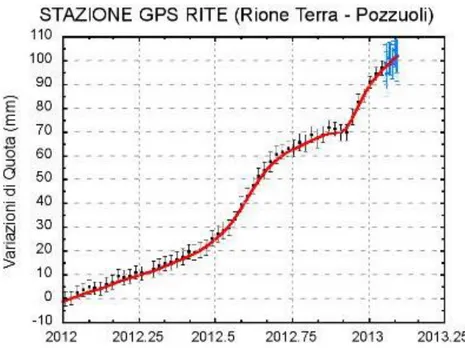
Figure 14 Variations of caposaldo n.25, in the Corso Umberto in Pozzuoli city, measured by geometric leveling (OV-INGV).

About the most recent activity in the Phlegrean area, geodetic measurements show a gradual uplift of the ground since 2008 (Figure 15). At the end of 2007, after a period of subsidence following the uplift of 2004-2006 (+ 4 cm), a new phase of uplift occurred, that has continued up through 2010 (average speed of +1 cm/year). Between April and June 2011, the vertical ground deformation rate increased up to 1 cm/month, after then it returned to the previous value. This evolution is well illustrated by the time series of the change in height for the GPS permanent station of RITE, located in Pozzuoli, in the maximum vertical deformation area (Figure 15).

There is an evidence also in the North and East component of GPS measures of ground deformation, in accordance with the inflation phenomenology of the Pozzuoli area during the 2008-2011 period (Figure 16).

(25)

25

Figure 15 Time series from 2006 of the vertical deformation in Pozzuoli, measured by the GPS permanent station (OV-INGV).

Figure 16 Planimetric displacements in the Phlegrean area in 2008-2011 period (OV-INGV).

About the seismicity, the Campi Flegrei area is characterized by a moderate activity that occurs mostly in swarms and during the deformation crisis the number and the magnitude of the seismic events increase.

Since 2000, 10 seismic crisis with swarms of earthquakes and some individual event occurred. In the beginning of 2011, 62 Volcano-Tectonic events were recorded with magnitude always less than 1 (Figure 17).

These earthquakes are mainly located in the Solfatara, the most active area in Campi Flegrei caldera.

(26)

26

Figure 17 Magnitude of seismic events from 2006 to 2011 (OV-INGV).

In the recent period the dynamic activity at Campi Flegrei caldera increased. Since the end of 2005 up to 2012 the vertical cumulative deformation recorded at the GPS-RITE (Rione Terra) station is of 21 cm (10 centimetres during 2012). The rate of ground deformation in 2012 suffered a rapid increase up to 5 cm/year (Figure 18). On September 2012, 219 earthquakes were recorded in the Campi Flegrei area and the rate of ground deformation reached a value of 1-1.6 cm/month. After this period the seismic activity and deformation went back to the values before this crisis, but at the end of 2012 there was a rapid increasing to 2-3 cm/month and a few number of seismic event. Also the geochemical activity underwent an increasing, mainly in the area of Pisciarelli vent, possibly due to the increasing of rainwater. In the first month of 2013 the ground deformation rate decreased to 1 cm/month (Figure 19) and the seismic activity went back to the background state with just a few small and shallow events recorded in the last months (OV-INGV, Bollettino mensile vulcani campani, 2012) (OV-INGV, Bollettino mensile vulcani campani, 2013).

(27)

27

Figure 18 Vertical ground deformation at the station RITE (Pozzuoli) since 2000 to 31st January 2013 (OV-INGV, Bollettino mensile vulcani campani, 2012).

Figure 19 Temporal series of vertical ground deformation at RITE station (Pozzuoli), since 1st January 2012 to 4th February 2013 (OV-INGV, Bollettino mensile vulcani campani, 2012).

(28)

28

4.2 The seismic network at Campi Flegrei

In order to monitor volcanoes, the principal use of a seismic network is the detection of signals associated to the volcano activity and correlated to the variations of its dynamic state.

Through the detection, analysis and interpretation of the seismic phenomena, the monitoring of volcanic processes aims to report the evolution of volcanic activity leading to a possible eruption in the short or medium term.

The Osservatorio Vesuviano (INGV) manages networks for seismic monitoring of the high risk volcanoes of Vesuvius, Campi Flegrei and Ischia which are high risk volcanoes because of their eruptive style, mainly explosive, and their proximity of large urban areas, and it also provides information on the seismicity at a regional scale measured by the Centralized National Seismic Network (INGV - National Center for Earthquake).

Figure 20 Seismic network of Osservatorio-Vesuviano, (OV-INGV)

The first reports of seismicity for a neapolitan volcano, Vesuvius area, date back to the second half of 1800 (the electromagnetic Palmieri seismometer – 1856).

In the second half of 60’s four stations were operating at the Vesuvius volcano, equipped with electromagnetic seismometers Hosaka and smoked papers records.

The first stations equipped with modern instrumentation (electromagnetic seismometers, frequency modulation, radio and telephone) date back to the early 70's.

(29)

29

Over the years, the Osservatorio Vesuviano Seismic Network was expanded both in number of stations, instrumentation and data acquisition systems. This enhancement has significantly lowered the detection threshold of the network, by doubling the number of localizable events and increasing the number of recorded signals with a high signal-to-noise ratio.

The complete seismic network that recorded the 2006 events at Campi Flegrei is in Figure 21 and consisted of:

 10 analogic stations, three components and short period;

 1 digital station, three components and short period;

 8 stations, three components and broad band;

 1 seismic antenna equipped with 5 sensors, three components and short period, plus 1 accelerometer.

The complete seismic network operating at Campi Flegrei area is illustrated in the following figure (Figure 21).

Figure 21 Map of Osservatorio Vesuviano seismic network operating at Campi Flegrei area (OV-INGV). Blue symbols refers to the permanent network and yellow symbols to the temporary one.

Stations equipped with short period sensor are marked with circles and the triangle are used for the broadband sensor stations. The circle with the black point inside refers to the array

(30)

30

5. The October 2006 seismic events at Campi

Flegrei

After the seismic swarm of October 2005, in October 2006 started a new seismic crisis, consisting of approximately 160 microearthquakes (M≤0.8) (Volcano-Tectonic events), recorded in the period from October 19th to 30th, 2006.

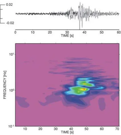
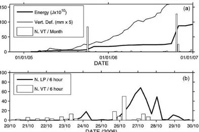
This activity was also followed by several hundreds of weak events with a monochromatic low frequency spectra, peaked at frequencies between 0.7 and 1 Hz. This events have a lack of clear S-wave arrival, a spindle-shaped waveform and were classified as Long-Period events. Their activity climaxed on October 27th, 2006, about one day after the most intense VT activity (Figure 22) (Saccorotti, et al., 2007).

Figure 22 (a) Number of VT earthquakes, energy release and ground vertical deformation in Pozzuoli, from GPS measurements. (b) Number of VT and LP earthquakes during 6 hours in the

20th-30th October 2006 crisis (Saccorotti, et al., 2007).

The last VT swarm occurred on December 21st, 2006, with highest magnitude of the entire period (M=1.4) .

The sources of most of the VT seismicity of October 2005 and October 2006 are clustered at depth spanning from 1 Km to 4 Km beneath the Solfatara crater. The origin of the December 2006 swarm is localized at depth from 1 Km to 2 Km under the Astroni crater.

Focal mechanisms, show a class of normal solutions with nodal planes rotating from N-S to NNE-SSW and finally to NNW-SSE (Saccorotti, et al., 2007).

(31)

31

About the Long Period events, several factors, as the absence of the same frequencies peaks in either the earthquake and the noise spectra, the presence of the same peak among all the stations of the network, suggest that they reflect a source effect.

The waveforms of the Long Period events can be grouped in three clusters (Figure 23) with similar locations along the S-E rim of the Solfatara at a depth of 500 m (Saccorotti, et al., 2007), (Figure 24).

Figure 23 Stacked velocity seismograms for the three clusters, from the NS component of station ASB2, individually normalised to their maximum amplitude (peak-to-peak) (Saccorotti, et al.,

(32)

32

Figure 24 Locations of the three clusters of LP events, superimposed to a map of the Solfatara Volcano (Saccorotti, et al., 2007). The three colors are relative to the three clusters of events

(Saccorotti, et al., 2007).

The monochromatic character of the LP oscillations and the similarity of the stacked waveforms suggest that this signal are generated by a non-destructive process of resonance, probably the harmonic oscillation of a fluid filled crack repeatedly triggered by very impulsive pressure boosts (Saccorotti,

et al., 2007).

To better understand the source of this low frequency seismicity and the characteristics of the fluids involved in the resonance processes, following the Chouet theory (Chouet, 2003) and using the power spectra of those LP, the quality factor of the resonator (different from the quality factor of the Earth medium) and the dominant frequency were estimated (Saccorotti, et al., 2007, Figure 25).

From the relationship (Eq. 3):

Eq. 3

where f is the frequency of the dominant spectral peak and Δf is the width of that peak at half of the peak’s magnitude, the quality factor Q of the resonator cavity could be obtained.

(33)

33

Using the radial components of the waveforms recorded at the ASB2 station (the one with the highest SNR), a quality factor peaked around the value 4 is obtained (Saccorotti, et al., 2007).

The values of Q could span over a wide range (10-500, from literature), reflecting the contrast of different physical properties between the multiphase fluid and the matrix of the surrounding rock (Kumagai, et al., 2002). In our case we can interpret the values of Q, in terms of a contrast of very low impedance at the fluid-rock interface preventing the trapping of elastic energy in the crack.

Figure 25 Dominant frequency (a) and quality factor (b) for the radial component of the LP events at station ASB2. Different tones correspond to event of different cluster (Saccorotti, et al., 2007)

Applying the measured quality factor to the crack-like geometry proposed by Chouet (Chouet, 2003) and considering the shallow depth of the LP source (500 m), the most likely candidate for the source process generating those LP events is a vibrating fracture filled with water vapour mixed with a low gas content (maybe the hydrothermal system of Solfatara volcano, extending over the 0-1500 m depth range) (Cusano, et al., 2008).

The crack length is between 40 m and 420 m, a size range which is consistent with the spatial spreading of the LP hypocentres (Cusano, et al., 2008).

Hence the October 2006 crisis can be explained in terms of fluid exchange between a deeper and a shallower reservoir beneath the centre of Pozzuoli (Battaglia M., et al., 2006). Possibly an overpressure in a cavity at 3-4 Km of depth containing fluids of magmatic origin, may have been caused a batch of magma rich in gas, from a deep source (Troise, et al., 2007).

This pressurization, in addition to the deformation, caused brittle failure in the above rigid layer, producing the VT events, occurring during the uplift phase.

(34)

34

The pressurization increased the permeability of the soil allowing the migration of the fluids and inducing the LP resounance events in the shallow hydrothermal system of the Solfatara (Saccorotti, et al., 2007). This caused an increasing of the temperature and velocity of the gases at the fumaroles (Cusano, et al., 2008) (Figure 26).

This scenario clarifies the role of the hydrothermal systems beneath the volcanoes: it induces ground deformations and LP activity and it amplifies the response to the arrival of fresh magmatic fluids from the depth.

Figure 26 (a) Daily average temperature (infrared measures) at Bocca Grande fumarole of Solfatara (solid line) compared with the steam velocity at the same place (grey dots). The values

are normalized. (b) Daily numbers of VT (black line) and LP (grey line) activity (Cusano, et al., 2008).

The scenario suggested for the October 2006 crisis is illustrated Figure 27 (Saccorotti, et al., 2007).

(35)

35

(36)

36

6. Data analysis – first step

In this chapter, the different steps of the analysis of the LP seismic data will be illustrated.

After the first step in which the waveforms and their characteristics will be studied, the different procedures adopted for the determination of the duration and the energy of that seismic events will be described.

In particular in the first step, the energy will be estimated through the envelope of the waveforms searching for a relation with their durations. During this phases lots of routines were developed to better understand the seismicity in order to quantitatively define the right parameters in the final analysis.

6.1 Preliminary analysis of the waveforms

In order to have the best data set possible, we chose the seismic stations whose waveforms presented the highest value of the SNR: ASB2, TAGG, AMS2, BGNB (Figure 28). The selected seismic stations are all equipped with digital 3C broadband velocimeters and they are localized near the epicentres of the events recorded on the October 2006 and analysed in this work ( see Figure 28).

Figure 28 Seismic network in the Campi Flegrei area. Highlighted in red are the stations whose waveforms are used in this work (OV-INGV).

(37)

37

The waveforms have been bandpassed using a ‘Butterworth’ filter, with 3 poles and 3 zeros, between 0.2 Hz and 1.2 Hz for the ASB2, AMS2 and TAGG stations, and between 0.5 Hz and 1.5 Hz for BGNB.

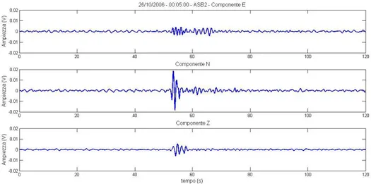
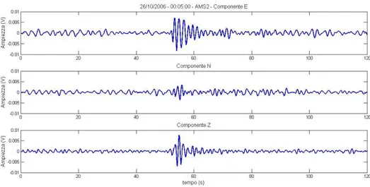
An example of 3C waveform for each station is reported in the Figure 29, Figure 30, Figure 31 and Figure 32, for the event recorded on October 26th 2006 at 00:05 at the four different stations. Hereafter we refer to this event as the "sample event".

Figure 29 Three components of the event recorded on October 26th 2006 at 00:05 at the ASB2 seismic station.

Figure 30 Three components of the event recorded on October 26th 2006 at 00:05 at the TAGG seismic station.

(38)

38

Figure 31 Three components of the event recorded on October 26th 2006 at 00:05 at the AMS2 seismic station.

Figure 32 Three components of the event recorded on October 26th 2006 at 00:05 at the BGNB seismic station.

Choosing waveforms with the highest signal to noise ratio (hereafter SNR), drastically reduced the number of treated events.

The analyzed LP seismicity (actually for the LP seismicity in general) is characterized by an unclear onset and end of the waveform. This evidence, combined with the low SNR, forced to develop a supporting function for manual detection of the onset of the seismic impulse, in addition to the formulation of algorithms useful to the identification of the duration (Section 6.2).

Observing the waveforms, could be noticed, in some components of each seismic station, a repetitive waveform occurrence, with amplitude often gradually lower than the first one (Figure 29, Figure 30, Figure 31, Figure 32). The presence of this kind of ‘sub-events’, even if it goes beyond this work, will be a little better studied in a dedicated Section (Section 6.4.2).

(39)

39

6.2 Duration of the events

Duration-magnitude scale are widely used in the volcanic observatories practice, generally to furnish quantitative evaluation of the energy associated to volcano-tectonic events. At first step, we were interested in trying to find a duration-magnitude calibrated scale for routine rapid estimations of the energy content for the LP seismicity too.

The differences of the LP’s waveforms respect to the tectonic seismicity involve also the difficulties in measuring their onset and their exact time duration. To achieve this goal different procedure have been developed. The duration of the LP was visually selected from the waveforms or from some supporting functions (root-mean-square (RMS) or amplitude-envelope), or automatically checked through two different routines based on the envelope or the RMS of the waveforms.

The three methods proposed will be discussed in the following paragraphs.

6.2.1 Duration – visually selection

It’s not easy to estimate the duration of a low frequency seismic event, due to its emergent onset and to the coda decaying masked into the noise.

Accordingly, we used two different supporting-function for the visual inspection of the waveforms, that helped us in this step of the study.

The first function has been derived by the method adopted in the dissertation of Petrosino, et al., 2007; it is based on the features of a function obtained through the Root Mean Square (RMS) of the signal.

We proceeded in the following way:

 each seismogram has been divided into many intervals of length 0.25 seconds. This duration window is chosen in order to reduce the noise-fluctuations that could masks the real trend of the final function.  for every time window the RMS was calculated (Eq. 4). So we obtained

a value of RMS every 0.25 s of signal.

√∑ Eq. 4

where yi is the waveform amplitude and N the number of the

(40)

40

 the value obtained for every time window was then multiplied by each value of the times of all the recording, obtaining a function which, for sake of simplicity, we will call RMST (Eq. 5).

(√∑ )

Eq. 5

where n is the indices of each point in the signal array.

The obtained curve is very helpful in selecting the duration of these events (Petrosino, et al., 2007); in fact, plotting Eq. 5 as a function of time, it shows a rapid increasing that corresponds to the impulse arrival and, after having reached a maximum, it decreases more or less rapidly until it reaches a minimum value, beyond which it starts to rise again. The time corresponding to this minimum, marks the end of the useful signal (Figure 33).

Figure 33 The function RMST (dotted line) calculated for the VT waveform in the lower panel (Petrosino, et al., 2007).

In fact, before the seismic arrival, the RMS is sensible to the background noise of the seismogram, so its amplitude is very low and even if multiplied by the time it won’t undergo major changes. On the contrary, after the arrival of the

(41)

41

signal, the value of the RMS, and consequently of the RMST, sharply increases.

Only after the end of the signal, the RMS resume very low values, which, however, multiplied by a growing time, and greater than those in the first part of noise (before the seismic impulse), are responsible for an increasing of the RMST function.

To better visualize the function RMST and minimize the fluctuations due to the noise, this function is applied to the waveform envelope. The envelope is calculated through the Hilbert Transform. Since the Hilbert Transform of a function has the characteristic of being out of phase with respect to the starting function (Figure 34), the envelope has been obtained by means of the following formula:

√

̅

Eq. 6

where represents the signal and ̅ is its Hilbert Transform.

Figure 34 Superposition of a signal (black line) and its Hilbert Transform (blue line).

Applying the function RMST to the envelope we were able to select the signal in each recording and to obtain, than, its duration; however sometimes the duration estimate was difficult due to problems in the identification of the end of the signal.

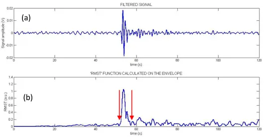
In Figure 35 an example of the seismogram and the related RMST function is illustrated.

(42)

42

Figure 35 (a) Waveform (filtered between 0.2 Hz and 1.2 Hz) of an event of 26th October 2006 at the ASB2 seismic station; (b) its function RMST. The red arrows correspond to the arrival time and

the end of the seismic impulse.

The second developed supporting-function is based on a kind of envelope of the waveforms. We decided to use an amplitude-envelope that refers to the changes of the waveform amplitude over the time. To develop it, we calculated the envelope linking the maximum of the modulus of the amplitude at several times. The complete array of the waveform was divided into intervals of a fixed duration. The time-step was chosen to “enough” reduce the noise fluctuations and to obtain a function that well approximated the waveform trend, at the same time.

For each interval the maximum of the modulus of the waveform amplitude was calculated and saved together with the corresponding time value. So we obtained an array of times correlated to the original ones (in this way, the comparison of the envelope with the original waveform was possible) and the corresponding values of amplitude envelope (See panel (b) in Figure 36 ). To better select the duration we denoised the envelopes subtracting the average of 10 seconds of noise envelope (the amplitude of the envelope several seconds before the seismic impulse) (see panel (c) in Figure 35). So we visually inspected the envelopes selecting the onset and the end of them and using these to determine the duration (panel (c) in Figure 36).

(a)

(43)

43

Figure 36 (a) Waveform (filtered between 0.2 Hz and 1.2 Hz) of an event of 26th October 2006 at the ASB2 seismic station, (b) its envelope, (c) the envelope denoised. The red arrows correspond

to the arrival time and the end of the seismic impulse.

In the definition of the amplitude envelope, the time interval, at which the maximum of the amplitude are selected, is very important, because a very short step doesn’t smooth enough the outline but, if it is too long it could hide the exact time to select.

Both the developed supporting-functions greatly helped us in the onset identification and duration selection, even though sometimes, to better mark the end of signals, the visual inspection of the original waveform was necessary.

6.2.2 Duration routines

In order to improve the previous procedures and make them usable in case of a large data set, we decided to develop some Matlab routines to determine the arrival time and the duration of the seismic impulse.

We decided to develop two routines based on different types of envelope: one obtained through the amplitude-envelope, and the other obtained through the RMS function.

First of all, these two routines were applied to the waveforms recorded at ASB2 since they showed the highest SNR of the entire data set.

6.2.2.1 Duration routine using the amplitude-envelope

This method is based on the calculus of the amplitude-envelope of the waveform (for the amplitude-envelope definition see Section 6.2.1).

(a)

(b)

(c)

(44)

44

The first step is to estimate the threshold to define the first arrival of the impulse. This is defined by computing the average amplitude value for 10 seconds of envelope at the beginning of the seismogram, where there is the contribution of only seismic noise. At this point, the routine scans the entire envelope and, the point for which the amplitude is larger than the threshold multiplied by a coefficient (greater than one) defined by the user, for more than a number of points defined by the user as well, is saved as the first arrival of the impulse. Then the routine continues to scan the envelope and, the time corresponding to an amplitude value lower than the threshold (multiplied by a coefficient different from the first one), for more than a number of points defined by the user, represents the end of the impulse. To avoid mistakes selecting the wrong impulse, the routine saves the waveforms only if their envelope maximum is not less than another threshold defined as the maximum of the envelope multiplied by a coefficient between 0 and 1.

This procedure was applied to each component for each event in order to have a large data set and make the statistical results more reliable.

The results are represented in Figure 37 (red dots).

6.2.2.2 Duration routine using root-mean-square

This routine follows the same steps of the previous one but, instead of the envelope, it uses the Root Mean Square (RMS) to analyze the waveforms. The RMS is calculated as described in the section 6.2.1.

Once calculated the RMS the routine works in the same manner as the previous method based on the envelope. So for the first step the threshold is estimated to define the first arrival of the impulse. This is defined by computing the mean of 10 seconds of the RMS at the beginning of the seismogram before the seismic impulse.

If the amplitude of the RMS, in the entire seismogram, is more than the threshold multiplied by a coefficient (more than one) defined by the user, for more than a number of points defined by the user as well, the corresponding time is saved as first arrival of the impulse. Then, if the RMS amplitude after the first arrival time, is less than the threshold (multiplied by a coefficient different from the first one) for more than a number of points defined by the user, the end of the impulse is defined.

Also in this case the waveforms are saved only if the RMS maximum is not less than another threshold defined as the maximum amplitude of the original waveform multiplied by a coefficient between 0 and 1.

(45)

45

A comparison between the results obtained through the two different routines is reported in Figure 37 where the results corresponding to each component of the ASB2 waveforms are represented.

The two envelope-routines are applied to each waveform and represented, on the same x-axes value, using two different colors (Figure 37): the blue dots for the amplitude-envelope routine and the red dots for the RMS routine. The integer numbers of the x-axes in Figure 37 represent the different events, each number refers to one event and for each of this, in the y-axes, the two different values of duration obtained by the different routines are shown. The results prove that different values of the duration can be obtained using different function, so, for this reason and for a good stability of the results, we decided to not use the routines showed in this section and we selected the duration visualizing the waveforms simultaneously with the amplitude-envelope or the RMST supporting functions (Section 6.2.1).

Figure 37 Comparison between the duration obtained through the two different duration-routines (using the amplitude-envelope (red dots) and the RMS (blue dots) of the waveform)

applied to the ASB2 waveforms. Each integer number (event index) on the x-axes refers to a different event.

(46)

46

6.3 Energy estimates – first step

The main purpose of this study is to estimate the magnitude of the low frequency seismic events. In order to achieve this goal, the first step is the estimate of the energy related to the LP seismicity. In the follow we will discuss the different methods adopted to calculate the energy of the LP events of October 2006 at Campi Flegrei caldera.

We used two different methods for energy estimation:

1. The first one is based on the calculation of energy through a theoretically obtained formula, depending on the amplitude of the waveform, on its dominant frequency and on parameters related to the propagation of the wave in the medium (propagation speed, density... ).

2. The second one is based on the calculation of the envelope of the waveform and of the relative area (once subtracted the background noise). This particular routine has been applied both to individual waveforms and to the average of the envelopes of the two horizontal components of each seismic event.

6.3.1 Energy via theoretical formula

This method has been used in the master thesis and modified through this work.

In order to obtain a big and statistical significant data set, all the components of each event have been used.

Considering a pointing source producing a wave train that propagates in every direction (Kasahara, 1981), we suppose that the seismic wave reaches the station at the epicenter (Figure 38) and we represent it using the displacement equation of the soil (Eq. 7):

( )

Eq. 7

(47)

47

Figure 38 Seismic wave arrival at the surface (Kasahara, 1981).

Consequently, the velocity is given by the time derivative of the displacement: ( )

Eq. 8

The kinetic energy density per volume unity , is then:

(

) ∫ ( ) (

) ∫ ( ) ( ) ( )

Eq. 9

where ρ is the density of the half-space, t0 is the duration of the wave-train

with n waves of period T0, and velocity c of the sound in the halfspace.

So, the energy flux per surface unit is: ct0 , and, if integrated on a h ray

surface (see Figure 38), we have the total kinetic energy at the origin:

( )

Eq. 10

Taking into account some considerations (Kasahara, 1981):

- the kinetic and potential energy are the same, so the total energy will be E= 2Ek ;

- the amplitude doubled at the epicentre (free surface), so a0=2a ,

where a is the wave amplitude at the hypocentre and a0 represents

the amplitude at the free surface;

- the previous calculations are for the S wave. The P wave energy is assumed to be half of the S one;

(48)

48

we obtain the following expression for the energy estimate:

( )

Eq. 11

where h is the depth in meters, t0 and T0 are, respectively, the duration and

the period in seconds, c is the velocity in m/s, a0 is the amplitude measured in

meters andρ is the density of the half-space in Kg/m3. For the LP studied, the wave velocity is 2000 m/s, the density 2000 Kg/m3 and the depth 500 m. To apply the Eq. 11 we used the dominant frequency obtained from the maximum of the amplitude spectrum, and the amplitude a0 obtained from

the maximum amplitude of the modulus of the signal (seismogram corrected taking into account the transfer function of the instrument).

First of all we applied this method to the ASB2 waveforms since they showed a better value of SNR, so, in Figure 39 the energy values are plotted versus the duration of the signal, in order to find a correlation between the two variables.

Figure 39 Energy vs duration for each component of every seismic event (semi-logarithmic scale) of the ASB2 seismic station, obtained using theoretical formula.

A non-correlation between energy and duration is evident in Figure 39. Just to confirm this results we calculated the correlation coefficient, that is -0.123. The modulus of this value is less than 0.3 so it reflects a non-correlation between the two variables.

(49)

49 6.3.2 Energy via envelope

The previous described approach about the energy evaluation (Section 6.3.1) is strongly dependent on the duration of the signal and on parameters typical of the area under study (propagation speed, density…). So, as second approach, we decided to evaluate a variable proportional to the energy of the signal using only some future of the waveform itself, such as the envelope. We assumed that velocity waveforms are representative of the kinetic seismic energy density at a specific location, and the potential energy density, for the equipartitioning of the energy, is equivalent to the kinetic one. This method is widely diffused in acoustic signal analysis, where the ‘relative energy’ associated to a signal is evaluated as the Measured Area under the Rectified Envelope (MARSE) (Lucas, McKeighan, & Ransom, 2001).

We calculated a variable proportional to the energy by integrating the seismic signal envelope over a time that corresponds to the entire duration of the transient. The envelope has been obtained connecting the maximum of the modulus of the waveform every fixed number of points (like in Section 6.2.2.1). The integral was calculated from the signal onset until the time that corresponds to the point where the amplitude returns less than the background noise.

In particular we applied this procedure in two different ways:

1. We calculated the envelope of every waveform, and then, for each of these we calculated the integral;

2. we calculated the average of the envelopes of the two horizontal components of each event (N-S and E-W) and for each of these we selected the duration and computed the integral.

6.3.2.1 Envelope of the single waveforms

For each waveform we calculated the integral for a selected time duration. We decided to select the duration visually inspecting both the waveform and the envelope.

First of all, we applied the envelope calculus on the filtered signal (Butterworth band pass filter between 0.2 Hz and 1.2 Hz for the waveforms recorded at the seismic stations ASB2, TAGG and AMS2; from 0.5 Hz and 1.5 Hz for the BGNB signals) to reduce the noise fluctuations. To avoid the contribution of the background noise we subtracted the average of 10 s of noise envelope (measured before the seismic impulse) to the entire envelope. In Figure 40 the waveform of the N-S component of the sample event recorded at the seismic station ASB2 is shown in the panel (a), in the panel (b)

(50)

50

the envelope is represented versus time and in the panel (c) the envelope after subtracting the ‘noise’ is plotted.

Figure 40 Waveform of an event filtered between 0.2 Hz and 1.2 Hz (a), envelope (b) and envelope corrected for the background noise contribution (c).

Once calculated the ‘denoised envelope’ we considered the duration obtained by a visual inspection of the waveform as well to calculate the integral. The obtained values are proportional to the energy of the events and are reported in the Figure 41 versus the time duration.

At this step of study, we decided to look at the results, showed in Figure 41 and following, obtained for the main impulses and these for the so called ‘sub-impulses’ separately (for a first explanation of the ‘main’ and ‘sub’ impulses see Figure 29, Figure 30, Figure 31 and Figure 32 in Section 6.1) (for a more accurately explanation of the main and sub impulses see Section 6.4.2), in order to eventually point out any different behaviour.

(a)

(b)

(51)

51

Figure 41 ‘Energy’ for each waveform versus duration of the event visually selected from the relative waveform. The blue symbols are relatives to the main impulse in the waveform, the red

one to the first sub-impulse and the green to the second one.

We also calculated the ‘energy’ from the envelope as illustrated before, using a time window selected from the envelope itself, and the results are showed in Figure 42.

Also in this figure we separated the values relatives to the different impulses.

Figure 42 ‘Energy’ for each waveform versus duration of the event selected from the envelope. The blue symbols are relatives to the first impulse in the waveform, the red one to the second

and the green to the third one.

We obtained similar results by selecting the time windows through a visual inspection of the waveforms or of the amplitude-envelope and, in both cases, a non-correlation between the two variables (‘energy’ and duration) is noticeable.