Design of wireless sensor networks for fluid dynamic applications

(1)

ALMA MATER STUDIORUM

UNIVERITÀ DEGLI STUDI DI BOLOGNA

________________________________

Dipartimento di Elettronica, Informatica e Sistemistica

Dottorato di Ricerca in Ingegneria Elettronica, Informatica

e delle Telecomunicazioni – XX CICLO

SSD: ING-INF/01 - ELETTRONICA

Design of wireless sensor networks for

fluid dynamic applications

Tesi di dottorato: Relatore:

Rossano Codeluppi Prof. Ing. Roberto Guerrieri

Coordinatore: Correlatore:

Prof. Ing. Paolo Bassi Prof. Ing. Marco Tartagni

______________________________________

Anno Accademico 2006 – 2007

(2)

(3)

To my family.

To Ale, Micky and Francesca .

To who hasn’t shared with me life and time in the last three years, but who has been always in my heart.

(4)

(5)

Keywords

Wireless sensor networks Capacitive pressure sensors

Fluid dynamics FEM Sensing Embedded system

(6)

(7)

Introduction

In fluid dynamics research, pressure measurements are of great importance to define the flow field acting on aerodynamic surfaces. In fact the experimental approach is fundamental to avoid the complexity of the mathematical models for predicting the fluid phenomena.

It’s important to note that, using in-situ sensor to monitor pressure on large domains with highly unsteady flows, several problems are encountered working with the classical techniques due to the transducer cost, the intrusiveness, the time response and the operating range.

For example sensors for aircraft design need high accuracy and precision, working in ranges up to ±2kPa. Otherwise the internal airflow sensor for automotive design requires a pressure operating range from ±10kPa to about ±30kPa. Considering sensors for nautical applications, they must detect pressure ranges up to only ±250Pa. A common specification in fluid dynamics applications is to create a measurement system able to work over a large size surface, using a large number of robust and conformable sensors so that the required spatial resolution is achieved. Certainly a real-time pressure measure is an important tool for the aerodynamic behaviour analysis of the body and its correct design. The required sensor properties will be: small dimensions, high rejection ratio to temperature, robustness , low cost and low environment-invasion level. The latter characteristic can be satisfied only if the whole measurement system is not invasive. In fact, each sensor need a read-out circuitry and there will be cables to collect data and to supply the structure, embedded inside the body under test.

The above specifications point out that the classical measurement techniques are suitable in laboratories where the aerodynamic surface are designed, but it’s rather unlikely to find them in the real environment where real bodies are used. An example can be to implement a classic pressure system on the top of a sail or on the racing car aerodynamic surfaces

To achieve a real and low invasive level it would be fundamental to remove every kind of wiring connection between the sensor and the device used to perform the data collection.

These remarks give the motivation to investigate the possibilities to change the classic sensor network implemented on the body under test in a sensor network based on wireless technology, without loss of robustness, number of measure points and real-time acquisition. Moreover creating a networks by means of wireless communication , on the top of aerodynamic surface is very challenging. In fact radio communication is an expensive energy process, the dedicated electronic increase the device dimensions and each measurement point must be a little system able to monitor the sensor, creating a digital data and managing a radio transmission.

The technological improvements of the last few years help to implement wireless communication. Wireless Senor Network platforms were born to perform an

(12)

environmental sensing (home control, security, health) but also are useful applications of the technology to allow exploring the technological challenges of further integration. Based on low power devices and miniaturized electronics, these structures are able to manage communications between sensors (set inside a wide area) and data collection point.

A interesting approach for satisfying the previously reported sensor requirements is the implementation of Micro-Electrical-Mechanical-Systems (MEMS). Using this devices small area occupation (tens of µm2) and the proximity of the read-out circuitry to sensor can be obtained permitting to improve the spatial resolution. However, aspects such as sensor packaging, time-consuming processes, robustness and costs cannot be neglected. In fact harsh environments or interfacial stress may be critical for the packaging procedure, limiting MEMS robustness.

The use of devices fabricated with polyimide or polyesters materials and assembled by means of micromechanical circuit board technology may represent a valid alternative to the MEMS solution, allowing sensors costs to be further decreased and providing features of environment-invasive-level and resolution fairly similar to the MEMS ones. Devices based upon the Printed Circuit Boards technology can be used for electro-mechanical transduction.

The purpose of this work is to design, build and test a sensor capable of acquiring pressure data on aerodynamic surface and to design and create a wireless sensor system able to collect the pressure data with the lowest environmental–invasion level possible.

The system is a network of electronics nodes able to sense pressure by means of developed sensor. The sensor is based on a flexible membrane changing the displacement because of fluid dynamics parameters variations. The membrane is an electrode of a capacitor, so that the displacement generates an electrical capacitance variation. The embedded electronics reads out such variations and translate them into a digital data and finally it transmits the information to a collection point. The wireless network must be able to manage several tens of nodes, guaranteeing a robust communication and a long life time of the system.

As a proof of concept, the monitoring of pressure on the top of the mainsail in a sail-boat has been chosen as working example.

(13)

Chapter 1

Fluid field measurement

Particular objects immersed in an ideal fluid and characterised by a geometry that determines a very small and attached vortical zone (non ideal fluid) are defined

aerodynamics and the vortical zone around them is defined as a boundary layer [1].

Example of aerodynamic object are the aircraft wings or the boat sails. When an aerodynamic object passes through the air, it creates a pressure gradient distribution, due to its geometry, velocity and due to the direction with respect to the air motion.

Fig.1.1 : Aerodynamic object moving through a real fluid

The boundary layer theory describes as if the boundary layer is sufficiently thin, there is no static pressure gradient, in the direction normal to the object surfaces: this means that the pressure just above the vortical zone is the same on the object surface. In this way, it is possible to obtain the pressure distribution at the object surface, using the Laplace and Bernoulli equations outside the boundary layer, on the aerodynamic object.

The aerodynamic loads acting on a body immersed in a flowstream are produced by the normal and tangential stresses over its surface due to the pressure distribution. When integrated, these stresses give rise to the resultant load components. These effects are strictly connected with the shape of the aerodynamic body.

It’s understandable how important the knowledge of these forces is.

An active control of the magnitude of pressure, over the surface of an aerodynamic object, is useful both for the design and for the basic concepts of fluid dynamics [2].

(14)

1.1 Pressure measurement background

Pressure can be acquired with different methods depending upon the applications and the required fluid dynamic conditions. The measurement techniques can be generally classified as direct or indirect, depending upon whether the instruments are able to measure the required physical quantity or evaluate it from other measured properties. A wide number of fluid dynamic techniques are available for describing the fluid flow behaviour. Mainly we can divide them by: MEMS devices, conventional pressure transducer and imaging techniques.

The MEMS pressure transducers operate a capacitive, resistance or piezoelectric transduction. They have an excellent spatial resolution and a real low invasive level but they are still expensive. The output accuracy of the MEMS, in fluid dynamic measurements, strongly depends upon a correct calibration as well as upon the conditions in which they are used (harsh environments are not suggested)[3].

The conventional transducers (i.e. Scanivalve®, Setra® Capacitive Instruments) use fluid dynamic probes, such as Pitot or Prandtl tubes to sense the flow field. They have an good spatial resolution but and they are very expensive with an high invasive level.

Finally the imaging techniques, as Pressure Sensitive Paint (PSP) or Optical measurements based on laser Doppler velocimetry can be used. This techniques have an excellent spatial resolution and a medium-high invasive level but they are still very expensive. Moreover the particular measurement setup is suitable only inside a laboratory.

The above remarks depict a technical scenario where is possible to perform excellent measures, investigating carefully the fluid field, but only laboratories are environments suitable to perform the measurements.

1.2 Proposed pressure measurement

Starting from reflections discussed in the last paragraph, it’s clear like, at moment, it’s impossible to perform real time experimental tests in the real environment where the aerodynamic body is used. This is an important technological gap.

In the present work we suggest a solution and we describe a system able to overcome the bounds of the current pressure measurements.

The goal is to create a sensors network to acquire pressure values in the real environment over an aerodynamic surface. The system have to be robust, reliable, with a low invasive level and operating in real time.

We have chosen to apply the sensor network on the surface of sail.

(15)

1.2.1 Measuring system description

To perform the pressure sensing on the top of a sail, in the real environment, is necessary to create a sensor network with the lowest invasive level possible. Every network sensitive point, composed by the sensor and read-out circuitry, must be very thin minimizing the total area. To be implemented on the sail, the sensor network have to remove every kind of physic connection. In fact, the sail is too thin and tens of sensors necessary hundreds of wires, disposed along the surface or embedded in the sail. It’s a quite complicated scenario.

The only solution is to perform a radio communication between every sensitive point and the network data collector. Therefore the sensitive point will be a wireless node housing the sensor, the sensing circuitry, the electronic dedicated to the radio transmission and node management, but also a power supply. The energy source has to be sufficient to allow node life time of several weeks

Fig.1.3 : system layout

The wireless sensor node will be a little system able to translate the data pressure in a digital information suitable to radio communication.

Wireless sensor nodes

PC Data

(16)

The sensor devoted to the application will be developed. The sensing will be done by the transduction of differential pressure between the sail leeward side and windward side (Fig.1.4) (an absolute sensor is not used because pressure variations on the sail are too small compared with atmospheric pressure) so an hole in the sail, below the sensor to create a static tap, will be necessary. Another opening, shaped like the sensor, must be created in the sail to allow the fluid field acting on the membrane sensor.

Fig.1.4 : pressure field detection

To obtain a low invasive level, the proposed wireless sensor network will be developed to be embedded in the sail battens. The wireless sensor node dimensions will be tuned on the batten shape and the number of nodes onboard each batten will be function of pressure map necessary (Fig.1.5).

a) b)

Fig.1.5 : a) example of node , b) batten instrumented

Finally the node will have to be flexible so that will be able to follow the sail curving.

1.3 Additional considerations

The measurement system proposed is devoted to perform a real time pressure monitoring on the top of a sail, operating in the real environment. It can be useful to

wind

Windward p2L p2W p3L p3W p4W p4L p1L Leeward p1W

(17)

trimming. Therefore the system can be an important means for analysis of the sail aerodynamic behaviour, helping the designer to optimize the aerodynamic object; otherwise it can be useful at the helmsman to improve sailing.

(18)

(19)

Chapter 2

Wireless sensor networks

The advances in radio frequency (RF) technology have created low-cost, low–power and multifunction miniature device. Low-cost, high performance RF devices and systems are finding their way in various applications. Some prominent applications include wireless LANs, portable GPS receivers, Bluetooth , RFID or wireless sensor networks (WSN). In particular WSN are applied to remote metering, home automation and large-scale sensor networks [4].

The wireless applications are classified by throughput and transmission range. If we compare the WSN with others applications, short range and low throughput are clear (Fig.2.1).

Fig.2.1 : comparison between WSN and others wireless applications

In fact, the wireless sensor networks have been created to collect sensors data ( few bytes) using limited energy (low power transmission), so that to implement the network over a wide region it will be necessary a huge number of sensor nodes. The architecture of the hardware sensor node consists mainly of five components: sensing hardware, processor, memory, power supply and transceiver (with antenna). Therefore the sensor node is able to sense, compute and actuate into the physical environments [5].

The wireless sensor networks can be an interesting solution to perform the wireless communication inside the proposed pressure measurement system.

(20)

2.1 Features

Operating into ISM (Industrial, Scientific and Medical) band ,the wireless sensor networks have several transmission frequency with different data rate (Fig 2.2). The transmission frequency is a very important parameter choosing the WSN platform suitable for the application, because it changes not only the data rate, but also the transmission range.

In fact, considering the Frijs transmission formula (2.1) that models the theoretical free-space loss between isotropic radiators in a communication system [6] , we have the relation between transmission frequency and power received into a transmission range. 2

4 











=

R

G

P

_R _T _T _R

π

λ

(2.1)

In the (2.1) PR is the received power, PT is the transmitted power, GT is the gain of the transmitting antenna, GR in the gain of the receiving antenna, λ in the operating wavelength and R is the distance between the TX and RX antennas. It’s clear as using the same transmission power but increasing the transmission frequency, it will be possible to obtain the same received power only into a shorter transmission range. The Fig.2.2 describes the available transmission frequency.

Fig.2.2 : ISM band : coverage, data rate and frequency

Changing transmission band, we find different data rate and the maximum is 250kbps. Therefore the WSN works with low data rate and this is a suitable characteristic of networks with low duty cycle like them . The sensor nodes can be active few tens of milliseconds over wide period like minutes or hours, because it has to monitor just a sensor. It’s important to note that low date rate allows to save energy and so it helps to have low power devices. In fact, to create a wide network with a large number of nodes, it’s necessary to have devices with long time life using common battery. To save energy, the wireless sensor networks have short transmission range (low PT) : 30-50metres indoor range, 100-200metres outdoor range. Moreover to have long battery life low power electronic is used Another important characteristic are the node dimensions: a small form factor is necessary to allows the system embedding it the operating environment so single chip with processor and transceiver embedded or miniaturized board are used[7] [8].

(21)

2.2 Network topologies

The wireless sensor networks are composed by two types of devices:

- Full Function Device (FFD) - Reduced Function Device (RFD)

The FFD are devices able to perform the data sensing but also to manage data routing inside the network. They are the routers or controllers network

The RFD are devices devoted to perform only the data sensing. They are the slaves device ( or network end points).

Every network needs at least one controller working like a network coordinator. There will be a large number of slaves able to communicate with the controller and, dependently from network topology, router can be used. The differences between the RFD and FFD are the amount of memory and the software programmed. In fact, the data routing functions are based on wide routing table (memorized) and a particular software management.

The WSN can have hundreds of network nodes, so it is important to find the best network topology to create the system. The three most common topologies are : star, mesh and hybrid.[9]

2.2.1 Star

In the Star topology all nodes (slaves) communicate directly with the network coordinator (Fig.2.3) . This type of network is very simple and the most suitable for short range applications.

Fig.2.3 : Star topology

The single-hop approach for communicating between each slave and the controller is the lowest overall power consumption [10]

2.2.2 Mesh

In the Mesh topology all devices are FFD. In fact, every node con communicates with all devices (into its transmission range). This is a multi-hop approach for

Node

(22)

communicating between each node and the controller. This topology is suitable to implement large-scale networks, with hundreds of nodes.

It’s energetically expensive and the transmission time is increased by each hop. In fact, every node employs some tens of milliseconds to transmits a received data. The communication is really robust, because each node can use many routes to reach the network coordinator.

Fig.2.4 : Mesh topology 2.2.3 Hybrid

The Hybrid topology mixes Star and Mesh topology. This is a multi-hop approach for communicating between each node and the controller, but not all nodes can transmit to every device into transmission range. In fact this topology is useful to shape network on the environmental geographic bounds. This topology is suitable to implement large-scale networks, with hundreds of nodes.

Fig.2.4 : Mesh topology FFD RFD

(23)

2.3 Network and Data management

To manage the wireless sensor networks it’s necessary a RF protocol. Nowadays the user can choose between two options: ZigBee protocol or a proprietary solution based on the RF standard IEEE 802.15.4. It’s important to note that not all WSN platform can use the two solutions, but just one is implemented. Usually the platform it’s chosen also dependently from used protocol [11].

The ZigBee solution is the WSN standard, and huge number of companies cooperate to develop it. Using ZigbBee the user creates a self-organizing sensor network, really reliable , flexible and easy to deploy [9]. This standard appears very interesting when a Mesh network with hundreds node has to be created over a wide area. If the network is small with tens of nodes creating a Star network, using ZigBee can be too complex.

Proprietary solutions, appear real interesting to develop a WSN simple or where the self-organizing property is not important [12]. In fact,programming the nodes is simple and faster than a ZigBee solution.

The RF protocol provides to the user an API ( Application Programming Interface) command data base necessary to develop the WSN management software.

It will be necessary to program the controller, the slaves and finally the router with devoted software.

It’s interesting to describe the basic methods to acquiring and propagating sensor data. There are three common classes: [13]

- periodic sampling : useful where the process needs to be monitored

constantly. Sensor data is acquired from a number of remote points and forwarded to a data collection center on a periodical basis;

- event driven : the sensor data is transmitted only when a certain threshold

is reached;

- store and forward : the sensor data is captured and stored by a remote

node before it is transmitted to the network coordinator.

The right method to acquire and propagate the sensor data is necessary to perform the best monitoring but also to minimize the power consumption. In fact, save transmission or power on the node only if necessary is basic to obtain long battery life.

2.4 The wireless sensor network chosen.

In the chapter 1 the measuring system is described. It’s clear that a wireless sensor network can be used to remove every cable and deploying a sensor network on the top of a sail. This is a shot-range application, because the nodes are deployed into a small area ( few tens of square metres) and the fastest communication between slaves and controller has to be performed. Finally the energy consumption is basic because the environmental bounds limit also the battery dimension.

Using the above remarks we have studied many platform based on ZigBee protocol or a proprietary solution. We have chosen a proprietary solution: the Z-WAVE™ platform by Zensys.

We have chosen Z-WAVE™ ZM0201 single chip solution because it was the first single chip on the market allowing to create a very small sensor node. In fact, into a

(24)

5x5mm QFN package there are a 8051 compatible microcontroller, a 868MHz RF transceiver, a 12 bit rail to rail ADC and ten configurable general purpose I/O pins. The power consumption is small : 2.5µA in sleep mode and 5mA n normal mode. The transmission power is programmable in the range -20dBm to 0dBm allowing to save energy in the transmission.

Finally it is interesting to note like in the Zensys developer kit are available different types of board to simplify the hardware and software test before the full customized electronic is created (Fig.2.5).

a) b) c) d)

Fig.2.5 : Zensys boards: a) ZW2106, b) ZW2106c, c) ZW2102, d) ZM0201

Working in the 868MHz ISM band Zensys platform allows to use less power to cover the same radio link compared with the 2.4GHz ZigBee solutions.

The very low data rate (9.6kbps) appears a limit , and so we will have to use carefully the available band.

(25)

Chapter 3

Design

and

simulation

of

Wing

Pressure Sensor

The strip pressure sensor for aeronautical use, described in the following section, has been developed in strict collaboration with other colleagues. In particular the project has been led off and developed by Dott. M. Zagnoni from the Phd thesis of whom [14] and Eng. A.Rossetti.

The author has been involved only in the sensor structure optimization, in the fabrication of sensor and in the test. The design and optimization of single sensitive unit have been performed by Mr. Zagnoni and Mr. Rossetti.

The performed activity, concerning the aeronautical pressure sensor, has been preparatory to be able to develop the sail pressure sensor, thus the behaviour of materials, the simulation methods and the fabrication technology are reported

The aeronautical pressure sensor is a conformable thin film strip, designed for aerodynamic applications. It is a capacitive differential pressure transducer aimed at monitoring the pressure profile on an aerodynamic body. Capacitive sensing has been chosen because of distinct advantages when compared to other, such as higher sensitivity, lower power consumption and better temperature performance. The differential pressure sensor approach has been preferred to absolute pressure sensors for overcoming altitude problems due to barometric pressure gradients.

The sensor was built using PCB (Printed Circuit Board) technology. This choice has been done because it allows the manufacture of the sensor by fast prototype machine directly into our laboratories so we obtained a technology independence in the development of the device. The materials used are perfect to achieve a good transduction by sensitive units created, and they allow to build a low cost device because cheap. Moreover, in the future, the PCB technology can allow the hosting of electronic sensing and signal processing components by means of smart packaging, (such as the chip on board) directly inside the sensor.

The proposed sensor is able to operate in a pressure field with the range of ±2000Pa and a resolution of units of Pa.

The device developed must be suitable for conforming to the profile surface and must be characterised by a total thickness that will not alter the fluid flow condition. This requirement is satisfied if the sensor is comprised within the boundary layer of the profile.

(26)

3.1 Sensor working principle

The pressure sensor system presented, is meant to produce an electric output related to the pressure distribution that is applied to the sensor strip surface. The fluid dynamic variables act on the deformable part of the sensors, where an electrode is placed, which, changing its geometry, leads to an electrical capacitance variation (Fig.3.1).

The latter can be electronically read in order to collect a set of surface pressure points, through a multiplexed switch capacitor sensing scheme.

Figure 3.1: Differential pressure sensor strip principle of operation. Membranes

deflect upward or downward with respect to the gradient of pressure between the outside and inside of the chamber.

As illustrated in Fig.3.1, the membrane at each point of sensing deforms itself downward or upward with respect to the static pressure reference taken by means of the holes. Since the membrane area is usually much smaller than the aerodynamic surface to be monitored, the corresponding pressure distribution over the deformable film can be considered constant with a good approximation, however the importance of the surface occupation of every sensing element in terms of spatial resolution becomes evident.

(27)

An application example is to investigate the pressure distribution over a wing profile. It depends on free stream velocity V and angle of attack α: a variation in the (α, V ) field leads to a different pressure pattern (Fig.3.2).

3.2 Sensor structure and optimization

3.2.1 Original sensor structure

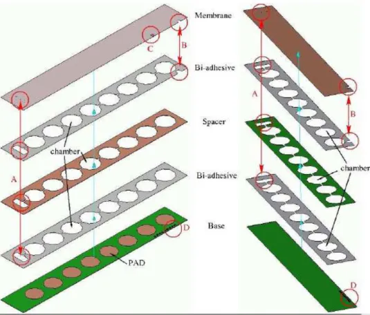
The sensitive unit consists of a three layer structure in a stack: Base, Spacer and Conductive Membrane (Fig.3.3):

- the Base layer is a rigid copper-clad glass-fibre composite layer. This layer hosts as many pads as pressure measurement points. Pads represent the lower plate of every capacitor (fixed electrode).VIAs (particular D) enable the addressing of every pad through the connection to a flat cable;

- the Spacer layer is a rigid glass-fibre copper-clad composite layer which is glued both to the top of the base layer and to the bottom of the membrane layer, forming the cavity within the membrane is deflected by the pressure input. All unity chambers are connected by miniaturised pipes, patterned in the spacing layers, in order to share the same internal pressure, forming a unique bigger chamber.

- the Membrane layer is a 25 µm thick deformable copper-clad (17 µm) Kapton® polyimide composite layer. Small holes (particular A) are drilled on the proximity of one the ends of the sensor, before the first sensing element and act as a pressure reference. A VIA (particular C) is designed for the connection of the upper electrode, through the same flat cable used for connecting the Base.

Layers are attached to each other by means of some 50 µm thick bi-adhesive tape, patterned in the same shape as the spacing layer. As shown in particular A of Fig. 3.3, a small chamber is realized for allowing the pressure reference to be shared in every sensing element chambers.

Exist also a copper layer acts as a guard ring, for reducing the coupling effects between the upper electrode on the membrane and the routes, on the top of Spacer. Particular B and C show how the spacer guard ring and the membrane can be electrically connected.

The device length and width can be set according to the application: the measurements and simulations reported here in this work are related to devices that are from 13 to 16 cm long and from 1.8 to 3 cm wide. The total thickness is comprised within 700 µm and 1 mm, as shown in Fig.3.4.

(28)

Figure 3.3: Pressure sensor strip structure: exploded top view (left side), exploded

bottom view (right side).Membrane, spacer and base are connected by means of bi-adhesive layers. A: small chamber for allowing the pressure reference to flow in the

spacer chamber. B: spacer guard ring electrical connection. C: membrane electrical connection. D: base electrical connections.

(29)

3.2.2 Layout optimization

The sensor has been built using PCB (Printed Circuit Board) technology. This choice, allowing the manufacture of the sensor by fast prototype machine directly into our laboratories, let to reach a technology independence in the development of the device but also it needs to pay attention during the design. In fact, not all manufacture solutions will be possible.

The sensor design depicted above showed some critical characteristics:

1) there is a guard ring ground connected in front of moveable electrode divided by bi-adhesive layer. If Spacer shape process (milling of rigid glass-fibre copper-clad covered by bi-adhesive layer) is not perfect, we can have small rips in the bi-adhesive and so creating short cuts between guard ring and membrane;

2) the guard ring contact is on the top side of sensor. The VIA is critical to solder because Kapton® surrounds and it breaks the flatness around the VIA area;

3) the electrical routes are on the top side of Base layer around the fixed electrode (Fig.3.5). The Base-Spacer junction, created by a 50um bi-adhesive, can be dangerous for sealed cavity within the membrane is deflected by the pressure input. In fact the un-flatness of the Base layer can create small pipes around electrical routes and connecting the inside chambers with external pressure. The pressure shared in every sensing element chambers could be different from the pressure reference.

Figure 3.5: top side of Base layer in the original pressure sensor

To avoid critical features we have changed the Base layer and simplify the Spacer layer.

To obtain a perfect flatness around the fixed electrode, we have translated the electrical routes in the bottom side of the Base layer (Fig.3.6). To perform the electrical connection with the fixed electrodes on the top side we have created a drill plated in the centre of each pad. To note that the drill plated is a pipe to external

(30)

environment: we have provided a cover by a Kapton® layer on the bottom side of the Base layer to close every drill.

Figure 3.6:bottom view of the Base gerber file

The second change has been to remove the guard ring from the Spacer layer and to translate it on the top side of the Base Layer (Fig. 3.7). This solution avoid every short cut chance between membrane and guard ring, and it removes the problem about the electrical connection. In fact, having the guard ring on the top of the Base layer a simply VIA is sufficient to lead the electrical contact on the bottom side, simplify the soldering. All electrical contacts will be in the bottom side of the Base layer.

Figure 3.7:top view of the Base gerber file with guard ring (red part)

The Spacer layer will have the same shape but without guard ring. The Membrane will not need the particular B of Fig. 3.3.

(31)

3.3 Designing methodology

3.3.1 Mechanical model compared with FEM simulation

The first designing step has been to develop an analytical sensor model for modelling the sensor and for identifying the parameters.

A cylindrical structure has been chosen for the sensing element. Such geometry considerably simplifies the model description, since a three dimensional axial symmetric configuration can be easily expressed in two dimensions, allowing much simpler equations to be considered both for the mechanical and the electric model representation.

The mechanical model is based on the classical mechanical theory of large deflection where a linear stress-strain relationship for matters (Hooke’s law) describes the linear displacement of plates with respect to the exerted pressure.

Afterwards Finite Element Method Simulations (FEM simulation) have been performed.

Aim of FEM simulations is to describe more efficiently the physical and structural sensor features, because of the sensor analytical formulation the behaviour might be not sufficiently accurate. To achieve a good design of the device due to the non linearity present both in the pressure-deflections transduction and in the electric capacitance relationship, other approximations are then introduce by means of the model used in the rule of mixtures, these topics lead to a non neglegible error in the capacitance integration.

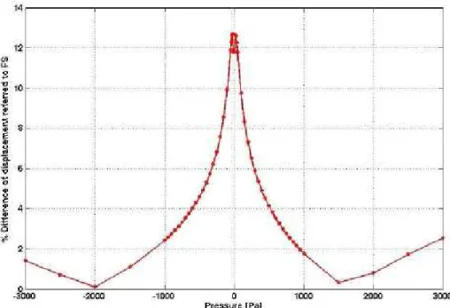
Studying the result of comparison between FEM simulation and analytical model, the latter appears unsuitable to design the sensor, as Fig 3.8 and 3.9 show.

(32)

Figure 3.9: difference (%) of displacement between analytical an FEM simulation

3.3.2 Creep : viscoelastic phenomena

Some materials subject to an external load can be considered, in the range of small deformations at ambient temperature whenever the internal stresses don’t exceed the yield and therefore can be treat as linear elastic solids. This assumption implies that the Hooke’s law can be used and that there is no time-dependent relationship between stress and strain. When a material is subjects to tension exciding the yield point or to lower tension but at high temperature then the relationship between stress and strain strongly depends on the size of the applied load, on the temperature, and crucially on time. This effect is usually referred to as viscoelasticity [15]. Materials as metals or ceramic manifest viscoelastic phenomena at very high temperature and load while other materials as polymers or polyester are still concerned with this phenomena at ambient temperature and low stress levels. An important implication of viscoelastic behaviours is that the stress-strain characteristic cannot be rigorously considered a static (i.e. memory-less, though nonlinear) relationship. Conversely, the stress-strain characteristic exhibits behaviours that appear highly non linear, even for small deformations, and that, most importantly, depends on the derivatives of the stress and strain functions. This phenomenon is well evidenced by the analysis of two cases.

(33)

Figure 3.10: Response to an applied constant stress.

As shown in Fig. 3.10, if a stress function step (σ0) is applied to a sample of material subject to creep, a sudden elastic strain is followed by a viscous and time dependent strain with an increasing trend (ε(t)). This phenomenon is referred as “compliancy” as is defined as: 0 ) ( ) ( σ ε t t D = (3.1)

Figure 3.11: Response to an applied constant strain.

Conversely, if a strain step is applied, the stress decreases as a monotonic function (Fig. 3.11) and is commonly referred as “relaxation”, defined as:

0 ) ( ) ( ε σ t t E = (3.2)

This type of behaviour is usually present in polyimides at ambient temperature and for stress bigger than 1 MPa [16] and is conventionally known as creep, where the common trends followed by materials are shown in Fig. 3.11. In viscoelastic material

(34)

the stress is a function of strain and time and so may be described by an equation of the form: ) , ( t f ε σ = (3.3)

This is known as a non-linear viscoelasticity, but as it is not amenable to simple analysis it is frequently approximated by the following form:

) (t f ⋅ =ε σ (3.4)

This response is the basis of linear viscoelasticity and simply indicates that for a fixed value of elapsed time the stress will be directly proportional to the strain.

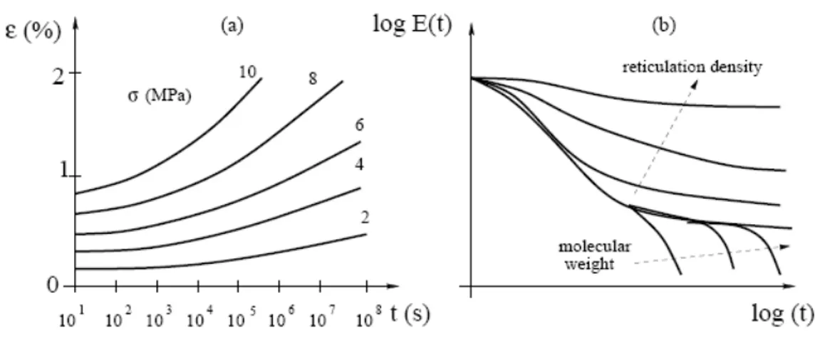
Figure 3.12: a) Creep deformation for different applied stresses. b) Qualitatively behaviour of the relaxation modulus as function of time and molecular structure.

However, this doesn’t imply that the time function is linear. First of all, it can be observed that the mechanical deformation of a body subject to creep phenomena is a function of the entire loading history of the body itself. In other terms, thanks to viscoelasticity the system gains memory: all previous loading steps contribute to the final response, as shown in Fig. 3.13.

(35)

Figure 3.13: Presumed creep response when different stresses are applied Creep affects the proposed structure, causing membrane deflections of some µm, manifesting themselves in time-scales of tens of minutes. The above observation implies that in order to know the exact response of a structure subject to creep, a model of its excitation should be available, describing the evolution in time of input stress (or strain). This is normally not possible in fluid dynamic applications where the input loading and its dynamic is unknown. In this case, the best that can be achieved is a bound on the maximal deviation that creep may introduce with regard to static models. Such bound can be roughly interpreted as an uncertainty that should be taken into account when using the sensor as a measurement device in a dynamic environment. A convenient way to obtain such bound consists of realising that creep can be approximately classified as a low-pass phenomenon, so that a typical ex-periment to estimate its extent consists of applying, at t = 0, a step-like excitation in stress spanning the whole allowable stress range and in evaluating the difference between the response at t = 0+ and the response at t →∞_{, where, of course, t}→∞ means a temporal value for which the experiment can be considered settled or the viscoelastic effect has reached more than 90 % of his relaxation behaviour.

The major reason to practise this kind of analysis is to understand how actions on the geometry and materials employed in the sensor fabrication can reduce the extent of the viscoelastic response and thus tighten the error bounds.

In the modelling of creep [17], the deformation model of a membrane changes from a static, non-linear, time-invariant model to a dynamic, non-linear, time-invariant model. In other terms, one could in principle model the viscoelastic behaviour by introducing time derivatives into the system of partial equations that rule the mem-brane deformation. In many conditions it is useful to model creep by using equations where time-varying parameters take care of describing the dynamical effects. A particularly effective way of doing so is by the introduction of a time dependent module of elasticity, obtained starting from Kapton®data sheets [16]. As shown in Fig. 3.14, from strain versus time curves, given by different applied stresses, the corresponding time dependent modulus of elasticity have been calculated, interpolating the strain curves, as:

) ( ) ( t t E i i εσ τ = (3.5)

where ε_i_{(t)is the time dependent strain,}σ_i_{is the corresponding stress and the index} “i” represents different values of stresses and temperature conditions. The approach

(36)

is convenient because it leads to equation sets which fit more easily into an analytical and conventional FEM simulation structure than models with explicit time derivatives. In other terms it allows creep to be obtained by a sequence of static simulations referring to different time instants. These curves (Fig. 3.14.b) have been fitted by :

(

)

i j t B ije k A t E ()=

∑

ij + τ (3.6)

where Aij , Bij and Ki parameters are representative of the elastic and viscous

be-haviour of the membrane in particular condition of exerted stress and temperature. The expressions obtained in Eq. 3.6 will be used for time dependent mechanical simulations and for analytical approximation in the design phase. The approach followed is an alternative and easier way to reproduce creep behaviour without differential equations, basing the estimation of the coefficients of Eq. 3.6 by means of interpolation, depending upon the stress and the temperature. Since the maximum membrane relaxation, due to creep, is obtained for the maximum pressure value, a time dependent capacitance variation can then be calculated until the transient response can be considered as finished or no longer relevant for the proposed application.

Figure 3.14: Kapton® creep: a) strain versus time behaviour from datasheet for particular temperature and stress conditions. b) time dependent modulus of elasticity Eτ_{(t), as described in Eq. 2.18 for particular temperature and stress conditions.}

(37)

3.3.3 Electro-Mechanical model compared with FEM simulation

The electric model has been developed considering the axial symmetry of the sensor and a parallel plate capacitor structure with electrodes of the same area The capacitance C is given by:

d A

C =ε (3.1)

where ε_{, A and d are the permittivity of the gap, the area of the plates and the} distance between the plates, respectively. For moving circular diaphragm sensor, the capacitance becomes: ϑ ε fdrd r w d C

∫∫

− = ) ( 0 (3.2)

where d0 is the distance between the plates when no pressure is applied and w(r) is

the deflection of the diaphragm . Due to the axial symmetry of the structure there is no dependence on the angle θ_.

Developing the expression 3.2 it’s possible obtain a math relation between sensor capacity and pressure applied in function of the membrane Young’s modulus E .The creep behaviour in the membrane is evaluated with a first order approximation, using two different values for the Young’s modulus, EMax and EMin.

The FEM simulation has been performed using modulus of elasticity Eτ_{(t) obtained} from Kapton®data sheets.

Figure 3.15: Electro-Mechanical model compared with FEM simulation As Fig.3.15 shows, the analytical and simulated methods presents a significant difference, especially for pressure values that lead the plates to get closer. The FEM

(38)

model remains a useful mean for a qualitative interpretation and it allows the designer to understand which effects are produced by changing the sensor parameters.

3.3.4 Conclusion

During the designing of sensor the best tool has been FEM model. It’s important point out that the design created without viscoelastic phenomena consideration (creep) appears unless. In fact, the creep change radically the behaviour sensor. Thus to perform a correct analysis we must to know modulus of elasticity Eτ_{(t); for the} wing pressure sensor we have used the Eτ_{(t) obtained from Kapton®}_{data sheets[16].}

(39)

Chapter 4

Fabrication of wing pressure sensor

For assembling the sensor we have chosen standard printed circuit board technology. This choice has been done because it allows the manufacture of the sensor by fast prototype machine directly into our laboratories so we have obtained a technology independence in the device development. The materials used are perfect to achieve a good transduction by created sensitive units, and they allow to build a low cost device because cheap.

Manufacturing the rigid part of sensor, fibreglass epoxy layers were used. They low thickness and stiffness guarantee both a low total thickness and a strong frame above which to stretch the membrane. The membrane is a Polyimide layer, a polymer commonly used for obtaining flexible connections in devices where a moveable part is utilised, i.e. inject printers, due to its resistance to cyclic stresses. Bi-adhesive tapes habe been used for assembling the three main parts of sensor (base, spacer and membrane).

4.1 Materials

4.1.1 Epoxy resin

FR4 laminate is the usual base material from which plated-through-hole and multilayer printed circuit boards are constructed. ”FR” means Flame Retardant, and Type “4” indicates woven glass reinforced epoxy resin. The laminate is constructed from glass fabric impregnated with epoxy resin and copper foil. Foil is generally formed by electro-deposition, with one surface electrochemically roughened to promote adhesion. FR4 laminate displays a reasonable compromise of mechanical, electrical and thermal properties. Dimensional stability is influenced by construction and resin content.

We used a two types of FR4 laminate:

- FR4 DURAVER-E-CU 104ML : 200 µm thick with copper 35 µm thick (both side) - FR4 DURAVER-E-CU 104ML : 125 µm thick with copper 17 µm thick (both side)

4.1.2 Polyimide

Polyimides are a very interesting group of incredibly strong and astoundingly heat and chemically resistant polymers, which are often used for replacing glass and metals, such as steel, in many demanding industrial applications. They can also be used in circuit boards, insulation, fibres for protective clothing, composites, and adhesives.

(40)

Aromatic heterocyclic polyimides are typical of most commercial polyimides, such as DuPont’s Kapton®. In this work we used:

- AKAFLEX KCL: a composite laminate made of a Kapton® VN layer and copper layer, whose thickness was 25 µm and 17 µm respectively, was used for the sensitive membrane.

- A generic 50 µm Kapton® layer : it was used like protective clothing of the sensor bottom side, where there are the electrical paths.

4.1.3 Bi-adhesive

We have used, for assembling the sensor layers, 3M Acrylic Adhesive 200MP in the format 7962MP. 200MP tapes are usually employed for bonding a variety of substrates, including most metal, sealed wood and glass, as well as many plastics. They are characterised by specific features such as high tensile strength, high shear and peel adhesion, resistance to solvent and moisture, low outgassing and conformability. The 3M Acrylic Adhesive 200MP in the format 7962MP is a 50 µm adhesive layer double coated by two 100 µm protective layers, presenting a total thickness of 150 µm (± 10% tolerance). It’s ideal for selective die-cutting.

4.2 Tools

The sensor fabrication consists of two steps: the first one produces the BASE, the SPACER and the MEMBRANE layer of the pressure sensors; the second step concerns to assemble the parts. Every layer is designed by CAD software and it’s created by PCB fast prototyping techniques. The layers have been bonded together by bi-adhesive films. To perform the layer bonding we have built a particular assembler device working with a vacuum table.

4.2.1 Fast prototype machine

To create every sensor layer the LPKF Protomat S62 fast prototype machine has been used.

(41)

This machine by means of milling tools, it’s able to draw, on a FR4 substrate or on other material (sheets of plastic, aluminium, copper) electronic circuit, and mechanical structures.

To use the fast prototype machine, we have created a project where the action of every machine tools are described by a dedicated software (CircuitCam) able to translate a generic CAD design in a project to be used by the prototype machine. To carry out the project we must use a particular management software (BoardCircuit): it creates the job machine which describes the number of devices and where the devices will be created, but it allows also the machine setup.

The LPKF Protomat S62 is a three axis (X,Y,Z) machine able to work with a maximum of 10 different tools in the same job, creating holes with different diameters and drawing lines of 100 um wide with a working precision of 10 um on the horizontal surface (X,Y). It isn’t a full 3D machine: in Z direction it’s possible to set only the tool working depth.

4.2.2 Assembler Device

The assembly procedure has been performed by means of special assembler built in laboratory of the faculty. The assembly device is presented in Fig. 4.2 a), it is composed by three floor of which just the middle one is movable. The bottom floor is fixed (Fig.4.3 a))on the ground and by means of three reference pivots allows the alignment of the base layer settle on it. The movable floor is actuated by a circular crank handle, and it houses also three reference pivots to perform the layers alignments . Moreover the movable floor is a suction surface, in fact it is connected, by means of a rectangular sealed chamber and a circle plug, to an extractor fan. It is thus possible to lay subsequently both the spacer and membrane layers to the movable floor, and to lower the floor to perform first the base–spacer junction and then the spacer-membrane junction to complete the assembly procedure. In Fig.4.2 b) the assembler device completely lowered is shown.

Figure 4.2 : a) assembler device sketch, b) created assembler device

Fix floors

Movable floor

Sealed suction chamber Crank handle

(42)

a) b)

Figure 4.3 : assembler device a) bottom floor, b) top and movable floor

4.3 Layers

The sensing unit is a three layers stacked structure:

- BASE : rigid part of the sensor built using a FR4 layer - SPACER : rigid part of the sensor built using a FR4 layer

- MEMBRANE : deformable part of the sensor built using AKAFLEX KCL The sensor vertical section is presented in Fig.4.4 : it’s possible to note the structure of every layer.

(43)

4.3.1 BASE

The BASE layer is an FR4 substrate covered by a double layer of copper. The copper thickness on each side of FR4 is 35um, the FR4 is 200um thick. After the creation of project by means of an electronic CAD, the sensor sketch is exported into the prototype machine management software.

a)

b)

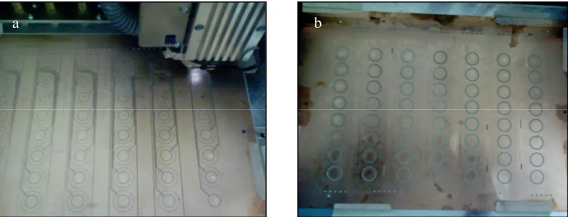
Figure 4.5 : Base gerber files: a) top view , b) bottom view

The fast prototyping machine area has been able to milling seven sensor layers at once (maximum working area is A4 size). The three different layers have been realized and bonded in the assembly procedure all at once, and subsequently divided by each others.

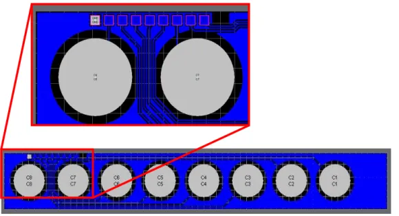
In the BOTTOM side of the BASE layer the electronic paths and the pads to carry out the electronic signals are present Fig.4.6 a). In the TOP side of the BASE layer the fixed electrodes of the capacitors are milled as shown in Fig.4.6 b). The signal of every fixed electrodes in the upper side, is routed to the electric paths on the bottom, by means of drills plated. It’s important point out that all fixed electrodes are enclosed by ground plane (shield) : it’s important to flat the junction surface between BASE and SPACER to obtain the best peel adhesion and to protect the fixed plate from electromagnetic interferences. The shield has been connected to ground by a devoted via near others fixed electrodes signal pads. Near the signal pads a square cut has been realized to allow the signal of the conductive membrane to be lead to the bottom side of the BASE through the thickness of the whole sensor. (Fig. 4.7)

Figure 4.6 : BASE layer: a)bottom side, signal routing, b)top side, fix electrode a

)

b )

(44)

Figure 4.7 : BASE gerber file: zoom of signal pads side

Drills holes between every internal cavity sensor and the external environment have been closed by means of a Kapton® layer set above the bottom side of the BASE, to avoid air to penetrate inside the cavity of every sensing unit. The Kapton® layer is also useful to preserve, the electronics path in the bottom side of the base, from oxidation (Fig. 4.8).

Figure 4.8 : Bottom side BASE sensor covered by Kapton® layer

4.3.2 SPACER

The SPACER layer is an FR4 substrate covered by a double layer of copper. The copper thickness of every layer is 17um, the FR4 is 125um thick. After the project creation by means of an electronic CAD, the sensor sketch is exported into the prototype machine management software.

(45)

Figure 4.9 : SPACER gerber files

All unity chambers are connected by miniaturised pipes, patterned in the SPACER layers, in order to share the same internal pressure, forming a unique bigger chamber. It’s possible to note that in the BASE gerber file, a square cut has been realized to allow the conductive membrane signal to be lead in the bottom side of the BASE through of the whole sensor thickness. (Fig. 4.9)

Figure 4.10 : SPACER layers covered by bi-adhesive

The SPACER layer is an FR4 substrate where the copper layers has been chemically removed, this layer when bonded to the base create the inner circle cavities where the circular electrode are present and the membrane is deflected. In order to create the internal chamber between the BASE and the MEMBRANE, the bi-adhesive layer has been bonded in upper and lower side of the FR4 SPACER layer before the milling process (without peeling off the remaining external coating protection). Acting in this way the spacer and the two bi-adhesive layers are shaped at once (Fig.4.10).

4.3.3 Membrane

The MEMBRANE layer is a 25 µm thick deformable copper-clad (17 µm) Kapton® polyimide composite layer (AKAFLEX KCL). After the creation of project by means of an electronic CAD, the sensor sketch is exported into the prototype machine management software.

(46)

Figure 4.11 : MEMBRANE gerber file

Three small holes are drilled on the proximity of one the ends of the sensor, before the first sensing element and acting as a pressure reference. The MEMBRANE was a AKAFLEX KCL sheet with the same dimension of sheet containing the seven SPACER layers.

4.4 Methods

4.4.1 BASE – SPACER bonding

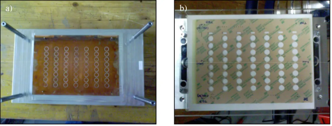
The BASE-SPACER bonding is performed aligning the sheet containing the seven BASE layer, above the fixed floor, of the assembler device, by the three reference pivot. The BASE layer is arranged to share the top side ( the one with the fixed electrode ) towards the movable floor (Fig.4.12 a)). The SPACER layer is aligned above the movable suction floor (Fig.4.12 b)), the bi-adhesive protective film is removed and subsequently the movable floor is lowered to perform the bonding process.

To obtain optimum adhesion, the bonding surface must be well unified, clean and dry. At room temperature, approximately 50% of the ultimate strength will be achieved after 20 minutes and 100% after 72 hours. In Fig.4.13 the BASE and SPACER layers are shown after the bonding process. The top side of the SPACER layer still present the bi-adhesive protection film, that will be removed in the following SPACER-MEMBRANE bonging.

Figure 4.12 : a) BASE layer above the fixed floor, b) SPACER above movable floor

(47)

Figure 4.13 : BASE and SPACER layers after the bonding

4.4.2 MEMBRANE – SPACER bonding

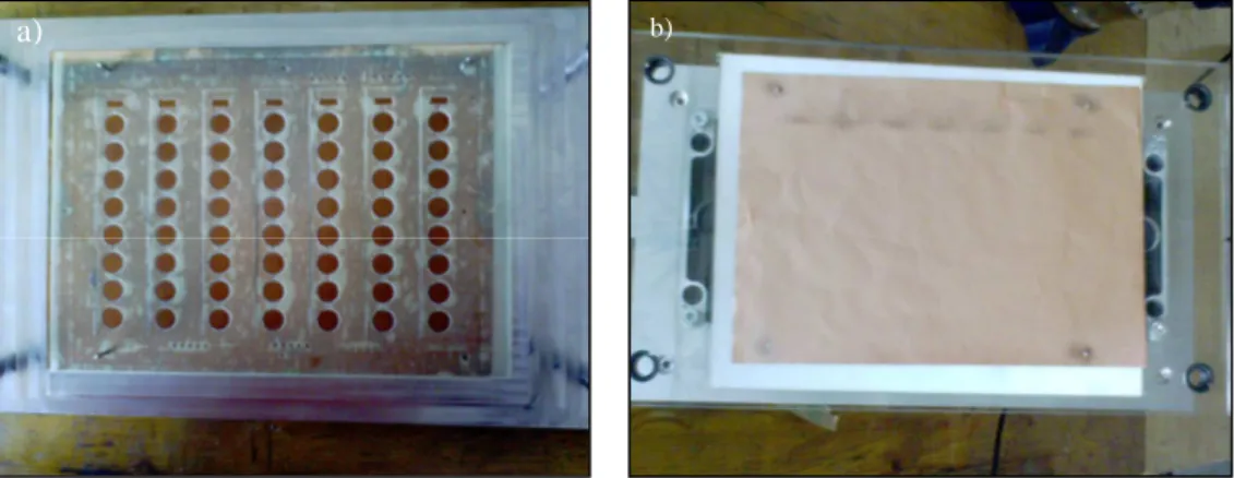
The MEMBRANE-SPACER bonding is performed aligning the previously bonded BASE and SPACER layers above the fix floor. The bi-adhesive protection film is removed from the upper side of the SPACER (Fig.4.14 a) ). The MEMBRANE layer is aligned above the movable floor and is arranged to share the bottom conductive side toward the bi-adhesive layer. The suction performed by means of the suction surface ensure the planar shape of the flexible membrane (Fig.4.14 b) ).

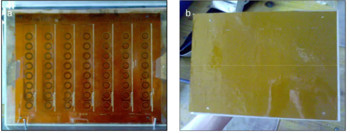
Subsequently the movable floor is lowered to perform the bonding process, in Fig.4.15 a) and b) the bottom and the top side of the assembled array of strip sensor are shown.

Figure 4.14 : a) BASE layer above the fixed floor, b) SPACER above movable floor

(48)

Figure 4.15 : assembled array of strip sensor a) bottom side , b) top side

Finally the array of strip sensor is aligned inside the PCB prototyping machine, to separate along the edge the single sensor unit. In Fig. 4.16 one of the final strip sensor is presented.

Figure 4.16 : final strip sensor - bottom side

The final size of strip sensor are: 158mm long, 22mm wide and only 0.6mm thick.

(49)

Chapter 5

Experimental results of wing pressure

sensor

The fabricated strip sensor in laboratory, as described in chapter 4, has been tested. The analysis set up intended to validate large deflections and creep simulation models for the sensitive unit in the array: this has been obtained by applying several pressure values (in the range from tens to hundreds of Pa) on the device membrane by means of sealed chambers that allow an independent measurement to be conducted on each sensing unit.

The test results have been compared to the first sensor series prototypes built by a PCB Swiss manufacturer, since in the laboratory where this work was originally developed, there were not the facilities for assembling the devices.[14]

5.1 Experimental setup

The experimental test targets were to obtain the static characteristics of the sensor and testing the long term behaviour of the sensor in order to depict the viscoelastic behaviour of sensor membrane. The setup to perform the tests is composed by:

- a wind tunnel, - a Pitot tube,

- sealed chambers for applying loads independently on the sensor membranes, - a conventional silicon-based pressure transducer,

- an LCR meter,

- a Labview® interface control system. The complete setup is shown in Fig. 5.1.

(50)

Fig 5.1 : the measure setup

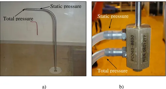
5.1.1 Wind tunnel and Pitot tube

A system composed by a wind tunnel and a Pitot tube has been used, to apply different pressure values on the membranes. Low pressure values, into a range of units to hundreds of Pascal, are very difficult to obtain statically acting on small volume variations. Indeed the temperature drift and of the pressure waves propagation create instabilities in the resulting thermodynamic pressure.

The problem depicted above has been avoided using, as referenced applied load, the dynamic pressure obtained from a Pitot tube in the wind tunnel test chamber inserted. Varying the wind tunnel free stream flow velocity, various pressure values can be achieved as the difference between the static pressure and the total pressure, as shown in Fig. 5.2.

a) b)

Fig 5.2 : Pitot tube a) into wind tunnel , b) output pressure channels

Total pressure

Static pressure

(51)

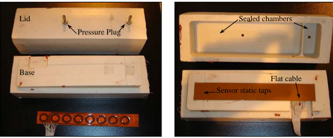
5.1.2 Sealed chamber

The sealed chambers for applying loads independently on the top of the sensor membrane has been built using PVC by means of a numeric-controlled milling machine in our laboratories. The PVC device is composed by a base (Fig. 5.3) where the sensor is leaned (like above an airfoil surface) and a lid where two sealed chamber have been milled. In the smaller sealed chamber by means of three static taps in the forward part of sensor, the reference pressure is led inside the internal chambers of all sensing units. In the larger sealed chamber a different pressure value is led, thus each sensing unit share the same differential pressure.

Fig 5.3 : sealed chamber

Every capacitor of the sensor is connected electrically to the measure instrument by a flat cable, soldered to the array.

5.1.3 Data read-out system

The conventional silicon pressure transducer, a Setra® Capacitive Instruments, connected to an National Instrument acquisition board, is used for measuring the pressure every time that the wind tunnel free stream velocity is varied by the dedicated control panel.

Fig 5.4 : Setra® Capacitive Instruments Lid

Base

Pressure Plug

Sealed chambers

Flat cable Sensor static taps

(52)

An Agilent 4284A Precision LCR meter has performed the data acquisition. The instrument is used for measuring directly the capacitance values to estimate the accuracy of the characteristic evaluated by the theory and by the FEM simulations. Data have been sampled by a National Instrument PCI-6070E High Performance 1.25 MS/s 12-bit multifunction acquisition board, controlled by a Labview program (Fig.5.5)

a) b)

Fig 5.5 : a) Labview programm ;B) Agilent 4284A Precision LCR meter

5.2 Static characteristic

A set of different constant pressure values have been exerted on the sensor membrane, each value being applied for an acquisition period of about sixty second , by mean of the sealed PVC chamber shown in Fig. 5.3. The static sensor characteristic and the creep drift was obtained by the modelling procedure described in chapter 3.

The fabrication process and the material employed are crucial issues in obtaining an reliable pressure sensing device; therefore a certain fabrication experience must be achieved. Tests on the first home made prototypes have shown a lack of repeatability in the static characteristic behaviour of the eight sensing unit of which the strip is composed (the results in Fig.5.6 are presented).

Fem upper bound

Fem lower bound

Nominal Fem characteristic

Design of wireless sensor networks for fluid dynamic applications

ALMA MATER STUDIORUM

UNIVERITÀ DEGLI STUDI DI BOLOGNA

________________________________

Dipartimento di Elettronica, Informatica e Sistemistica

Dottorato di Ricerca in Ingegneria Elettronica, Informatica

e delle Telecomunicazioni – XX CICLO

SSD: ING-INF/01 - ELETTRONICA

Design of wireless sensor networks for

fluid dynamic applications

Rossano Codeluppi Prof. Ing. Roberto Guerrieri

Prof. Ing. Paolo Bassi Prof. Ing. Marco Tartagni

______________________________________

Anno Accademico 2006 – 2007

Keywords

Contents

Introduction

Chapter 1

Fluid field measurement

1.1

Pressure measurement background

1.2 Proposed pressure measurement

1.3 Additional considerations

wind

Chapter 2

Wireless sensor networks

2.1 Features

4













=

R

G

G

P

P

π

λ

2.2 Network topologies

2.3 Network and Data management

2.4 The wireless sensor network chosen.

Chapter 3

Design

and

simulation

of

Wing

Pressure Sensor

3.1 Sensor working principle

3.2 Sensor structure and optimization

3.3 Designing methodology

(

)

∑

∫∫

Chapter 4

Fabrication of wing pressure sensor

4.1 Materials

4.2 Tools

4.3 Layers

4.4 Methods

Chapter 5

Experimental results of wing pressure

sensor

5.1 Experimental setup

5.2 Static characteristic