Development of innovative transducers based on Magnetic Fluids

(1)

NOTA: tagliare il blocco di pagine della tesi (stampata fronte-retro)

lungo le due linee qui tracciate prima di effettuare la rilegatura

NO

T

A:

an

ch

e

qu

es

ta

p

ag

ina

bi

an

ca

f

a

pa

rt

e

de

l b

lo

c-co

d

i p

ag

in

e d

ell

a te

si

(2)

(3)

UNIVERSITÀ DEGLI STUDI DI CATANIA

FACOLTÀ DI INGEGNERIA

D

OTTORATO DI

R

ICERCA IN

I

NGEGNERIA

E

LETTRONICA

,

A

UTOMATICA E DEL

C

ONTROLLO DI

S

ISTEMI

C

OMPLESSI

XXIV

CICLO

A

NGELA

B

ENINATO

Development of innovative transducers based on

Magnetic Fluids

Ph.D. Thesis

Tutor: Prof. Ing. Salvatore Baglio

Coordinator: Prof. Ing. Luigi Fortuna

(4)

(5)

(6)

(7)

Acknowledgements

During the period of my Doctorate I had the support of many people who contributed, in different ways, to the realization of this work.

First of all I would like to thank my guardian Angels, my parents, whose sacrifices allowed me to reach this important achievement, and my brother Danio, whose support was very important for me.

A very special thank to Alessandro, who always sustained and en-couraged me with love and patience and who believed in me and in this project. He stood by me in the most difficult periods of my life, helping me to overcome them. He was and he is my light in the dark. For all these reasons and for much more this Thesis is dedicated to him.

I want to say how grateful I am to Prof. Salvatore Baglio and Prof. Bruno Andò for the thrust they had in me and for all their lessons and

(8)

suggestions; they were an inexhaustible source of ideas, inspirations and enthusiasm, and I have learned a lot from them.

I would like to thank Prof. Luigi Fortuna, Coordinator of my Ph.D. course, for the opportunity he gave to me.

I want to say thanks to my colleagues Elena, Vincenzo, Carlo, Salvo and Gaetano for the several mutual information exchanges that have been very relevant to improve my knowledge, and for making my work-ing days very pleasant.

(9)

Preface

The investigation of new approaches and methodologies for the devel-opment of sensors and actuators is strictly related to the investigation of novel materials and technologies allowing for widening devices usability well beyond traditional fields of applications.

Actually, the use of novel materials can permit the development of sensing methodologies and readout strategies with interesting peculi-arities.

This Ph.D. thesis addresses the possibility to exploit magnetic fluids for the realization of innovative sensors and actuators. The use of such “shapeless” materials allows the synthesis of transducers with dramatic features especially in terms of reliability to mechanical shocks and ar-chitectural flexibility which opens the use of these devices to a wide range of real applications.

(10)

Above a general introduction on magnetic fluids and their standard applications, the thesis covers aspects related to innovative sensing strategies adopting a ferrofluid sample as the active inertial mass of the transducer. Novel ideas, design, models, simulations, implementation of lab-scale prototypes and their metrological characterizations are the main contributions of this Ph.D. Thesis.

The Thesis content is really deep and, although rich of already con-crete methodologies assessed by real working devices, in my opinion it represents a milestone in the context of ferrofluid transducers stimulat-ing further research activities in this field.

This Thesis resumes an intense research activity that Angela well conducted within the research group working in the sensor laboratory at the DIEEI in Catania. Reading this work evidences the original and valuable contribution of the author in the field of innovative transduc-ers using ferrofluids, her competencies and scientific maturity.

I would like to give to Angela my personal compliments for this ex-haustive and high level job and I wish the best for her future job and success for her life.

(11)

List of figures

FIGURE 1-1 A)RANDOM ORIENTATION OF ATOMIC MAGNETIC MOMENTS IN AN UNMAGNETIZED SUBSTANCE. B) WHEN AN EXTERNAL FIELD IS APPLIED, THE ATOMIC MAGNETIC MOMENTS TEND TO ALIGN WITH THE FIELD, GIVING THE SAMPLE A NET MAGNETIZATION VECTOR . ... 9

FIGURE 1-2 IN BULK FERROMAGNETIC MATERIALS DIPOLE ALIGNMENT IS SPLIT UP INTO DOMAINS. ... 10

FIGURE 1-3 MAGNETIC HYSTERESIS LOOPS FOR SOFT AND HARD MATERIALS ... 11

FIGURE 1-4 TYPES OF MAGNETISM: PARAMAGNETISM, FERROMAGNETISM, ANTIFERROMAGNETISM AND FERRIMAGNETISM. ... 14

FIGURE 1-5 BEHAVIOR OF THE MAGNETIC FIELD PRODUCED BY AN ELECTROMAGNET CENTERED IN WITH A RADIUS . 17

FIGURE 1-6 BEHAVIOR OF THE MAGNETIC FIELD PRODUCED BY A PERMANENT MAGNET CENTERED IN AND WITH A RADIUS

(16)

FIGURE 1-7 MAGNETIC FIELD SENSORS ARE DIVIDED INTO TWO CATEGORIES BASED ON THEIR FIELD STRENGTHS AND MEASUREMENT RANGE: MAGNETOMETERS MEASURE LOW FIELDS AND GAUSSMETERS MEASURE HIGH FIELDS. ... 22

FIGURE 2-1 SCHEMATIC OF FERROFLUID PARTICLES, WITH HIGHLIGHTED THE MAGNETIC CORE AND THE SURFACTANT. ... 27

FIGURE 2-2 EXAMPLES OF FERROFLUIDS SUBJECTED TO MAGNETIC FIELDS. ... 29

FIGURE 2-3 STRUCTURAL LATTICES FORMED IN A THIN LAYER OF THE MAGNETIC FLUID EXPOSED TO AN ALTERNATING ELECTRIC FIELD AT DIFFERENT FREQUENCIES: A)2 AND B) 10 . ... 29

FIGURE 2-4 VS , AND VS FOR EFH1 FERROFLUID. ... 38

FIGURE 2-5QUALITATIVE BEHAVIOR OF THE MAGNETIC FORCE PRODUCED BY AN ELECTROMAGNET. ... 41

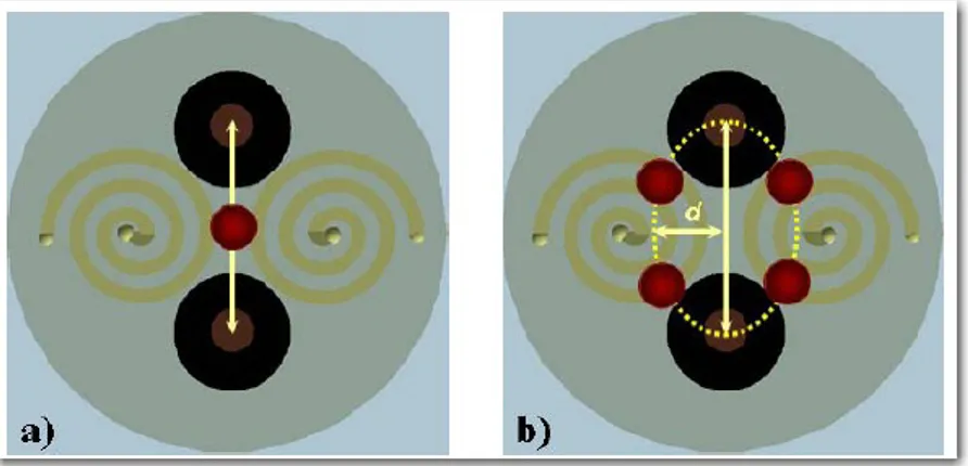
FIGURE 3-1SCHEMATIZATION OF THE FERROFLUID GYROSCOPE. ... 45

FIGURE 3-2 SCHEMATIC OF THE MOTION OF THE FERROFLUID MASS A) WITHOUT ANGULAR RATE AND B) WITH ANGULAR RATE.THE DISTANCE D DEPENDS ON THE ANGULAR RATE AMPLITUDE ACTING ON THE SYSTEM.

... 46 FIGURE 3-3BLOCK DIAGRAM OF THE DRIVING ELECTRONICS. ... 47

FIGURE 3-4SCHEMATICS OF THE READOUT SENSING ELECTRONICS. ... 48

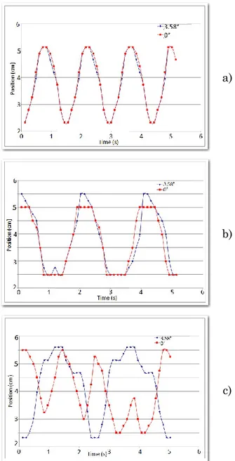
FIGURE 3-5 A TYPICAL FRAME AND THE SUPERIMPOSED GRID WITH A RESOLUTION OF . ... 51 FIGURE 3-6TIME EVOLUTION OF THE FERROFLUID MASS ( ) POSITION FOR A DRIVING SIGNAL OF: A) @690 , B) @500 C) @ , AND FOR TWO DIFFERENT TILTS.CASES B) AND C) ARE EXAMPLES WHERE THE FERROFLUID MASS FAILS TO FOLLOW THE DRIVING SIGNAL. ... 52

FIGURE 3-7 DRIVING PARAMETER MAP HIGHLIGHTING THE OPTIMAL WORKING REGION (TILT=0°). ... 53

FIGURE 3-8REAL VIEW OF THE SENSOR ARRAY USED FOR THE ESTIMATION OF THE ELECTROMAGNETS FIELDS. ... 54

FIGURE 3-9 SCHEMATIZATION OF THE SENSOR ARRAY USED TO MEASURE THE GENERATED MAGNETIC FIELDS. ... 55

(17)

Indexes vii

FIGURE 3-10 SPATIO-TEMPORAL BEHAVIOR OF THE MAGNETIC FIELD MEASURED ALONG THE DRIVING AXIS DUE TO ONE ELECTROMAGNET. . 55

FIGURE 3-11 EVOLUTION OF THE MAGNETIC FIELD AND THE MAGNETIC FORCE ALONG THE DRIVING AXIS. ... 56

FIGURE 3-12 TIME EVOLUTION OF THE MAGNETIC FORCE, THE MAGNETIC FIELD AND THE FERROFLUID MASS POSITION A) IN A GENERIC POINT ALONG THE DRIVING AXIS, AND B) IN THE LOCATION OF ONE ELECTROMAGNET. ... 57

FIGURE 3-13 BEHAVIOUR OF THE MAGNETIC FIELD AND THE MAGNETIC FORCE ALONG THE DRIVING AXIS FOR THE SPECIFIC TIME SLOT WHERE THE MAGNETIC FIELD AMPLITUDE REACHES ITS MAXIMUM VALUE

(SCALING FACTORS GIVEN IN THE VERTICAL AXIS LABEL HAVE BEEN USED FOR THE SAKE OF CONVENIENCE). ... 58

FIGURE 3-14MODEL OF THE NUMERICAL INTEGRATION ADOPTED. ... 59

FIGURE 3-15 COMPARISON BETWEEN THE EXPERIMENTAL AND THE PREDICTED EVOLUTION OF THE FERROFLUID MASS. ... 60

FIGURE 3-16 SIMULATION RESULTS OF THE MASS TRAJECTORY INTERSECTIONS WITH THE Y AXIS AS A FUNCTION OF THE IMPOSED ANGULAR RATE. ... 61

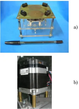
FIGURE 3-17 EXPERIMENTAL SET-UP ADOPTED FOR THE DEVICE CHARACTERIZATION; A) SENSING-DRIVING SYSTEM AND B) STEP MOTOR.

... 63 FIGURE 3-18CALIBRATION DIAGRAM OF THE FERROFLUID GYROSCOPE. .. 64

FIGURE 3-19 SCHEMATIZATION OF FORCES ACTING ON THE FERROFLUID MASS: IS THE MAGNETIC FORCE, IS THE GRAVITATIONAL FORCE AND IS THE HYDROSTATIC FORCE. ON THE LEFT HAND SIDE THE STEADY STATE REGIME IS SHOWN; ON THE RIGHT HAND SIDE AN EXTERNAL STIMULUS PERTURBS THE SYSTEM AND THE FREE-END OF THE FERROFLUID SPIKE CHANGES ITS POSITION. THE DIODE USED TO PRODUCE THE IR EMISSION IS REPRESENTED WITH FOUR YELLOW AND SYMMETRICALLY ARRANGED CIRCULAR RING SEGMENTS, WHILE THE PHOTODIODE IS REPRESENTED WITH A FILLED YELLOW CIRCLE. ... 66

FIGURE 3-20 BLOCK DIAGRAM OF THE READOUT STRATEGY. THE FIRST BLOCK IN THE LEFT-HAND SIDE IS THE PIPETTE WITH THE SPIKE SHAPED FERROFLUID MASS; THE SECOND BLOCK REPRESENTS THE

(18)

CONVERSION BETWEEN THE FERROFLUID DISPLACEMENT AND THE IRRADIATED AREA OF THE IR DEVICE; THE LAST BLOCK IN THE RIGHT -HAND SIDE REPRESENTS THE IR DEVICE. A VOLTAGE TO CURRENT CONVERTER WAS USED TO DRIVE THE IR TRANSMITTER, WHILE A STANDARD VOLTAGE DIVIDER WAS USED TO OBTAIN AN OUTPUT VOLTAGE FROM THE IR DEVICE. ... 68

FIGURE 3-21 SCHEMATIZATION OF THE INTERACTION BETWEEN THE FERROFLUID SPIKE AND THE IR DEVICE. ... 69

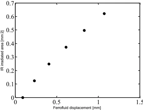
FIGURE 3-22 THE RELATIONSHIP BETWEEN THE DISPLACEMENT OF THE FERROFLUID SPIKE (FREE-END) AND THE IRRADIATED AREA.A LINEAR FITTING BY MODEL PRODUCES AN ESTIMATED RESIDUAL OF 0.008 . ... 70

FIGURE 3-23 A) REAL VIEW OF THE DEVICE; B) ZOOM OF THE FERROFLUID SPIKE; THE IR EMITTER DIODE IS REPRESENTED BY A DOTTED CIRCLE WHILE THE PHOTODIODE IS REPRESENTED BY A FILLED WHITE CIRCLE.

... 72 FIGURE 3-24 CONDITIONING ELECTRONICS USED FOR A) DIODE AND B) PHOTODIODE. ... 73

FIGURE 3-25 EXPERIMENTAL SET-UP FOR THE DEVICE CHARACTERIZATION. ... 74

FIGURE 3-26FREQUENCY RESPONSE OF THE SHAKER. ... 75

FIGURE 3-27FREQUENCY RESPONSE OF THE DEVICE. ... 75

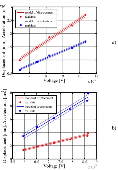
FIGURE 3-28 CALIBRATION DIAGRAMS FOR STIMULI A) @4 AND B) @8

.DOTTED LINES REPRESENT THE UNCERTAINTY BAND ESTIMATED. 77

FIGURE 3-29SCHEMATIZATION OF FLOW SENSOR. ... 80

FIGURE 3-30 CONDITIONING ELECTRONIC FOR THE INDUCTIVE READOUT STRATEGY. ... 80

FIGURE 3-31THE FERROFLUID SPIKE INSIDE THE PIPE FOR A) NULL FLOW RATE AND B)0.3 .THE MASS OF FERROFLUID CHANGES ITS SHAPE DUE TO THE TIP MOVEMENT ... 82

FIGURE 3-32THE FERROFLUID SPIKE INSIDE THE PIPE FOR A) NULL FLOW RATE, B)1 AND C)1.7 . THE MASS OF FERROFLUID CHANGES BOTH ITS SHAPE (TIP DEFLECTION) AND POSITION. ... 83

(19)

Indexes ix

FIGURE 3-33 BEHAVIORS OF THE FERROFLUID SPIKE TIP DISPLACEMENT,

X, AS A FUNCTION OF THE FLOW RATE INTENSITY FOR DIFFERENT VALUES OF THE RETAINING MAGNETIC FIELD. ... 84

FIGURE 3-34 TWO TYPICAL FRAMES FOR THE ESTIMATION OF THE FERROFLUID SPIKE TIP POSITION. ... 85

FIGURE 3-35SIMULATED FREQUENCY RESPONSES OF THE DEVICE. ... 88

FIGURE 3-36 SIMULATED STEP RESPONSES (FOR Q=1 ) OF THE DEVICE. ... 88

FIGURE 3-37 A) REAL VIEW OF THE FLOW SENSOR; B) EXPERIMENTAL SET -UP ADOPTED TO CHARACTERIZE THE SENSOR PROTOTYPE... 90

FIGURE 3-38THE SENSOR RESPONSE FOR RETAINING MAGNETIC FIELDS OF

133G,153G AND 186G. ... 90

FIGURE 3-39 SCHEMATIZATION OF THE DEVELOPED TDR INCLINOMETER.

... 94 FIGURE 3-40BLOCK DIAGRAM OF THE SENSOR WORKING PRINCIPLE. ... 96

FIGURE 3-41 QUALITATIVE BEHAVIOR OF THE SIGNAL MODULATION DUE TO THE MASS MOVEMENT: . ... 98 FIGURE 3-42 A SCHEME OF THE ELECTRONICS USED TO DRIVE THE ACTUATION COIL. ... 99

FIGURE 3-43 A SCHEME OF THE ELECTRONICS USED TO SENSE THE MASS POSITION. ... 99

FIGURE 3-44REAL VIEW OF THE DEVELOPED PROTOTYPE. ... 101

FIGURE 3-45 SNAPSHOTS OF THE REALIZED INTERFACE: A) CONTROL OF THE TILT, B) COMPARISON OF THE OUTPUT SIGNAL WITH THE TWO THRESHOLD VALUES AND MONITORING OF THE SIGNAL PROCESSING, C) ACQUISITION OF THE OUTPUT DATA. ... 103

FIGURE 3-46 OUTPUT SIGNALS OBTAINED IMPOSING DIFFERENT TILT VALUES. ... 105

FIGURE 3-47 COMPARISON BETWEEN TWO OUTPUT SIGNAL WITH CONSECUTIVE VALUES OF IMPOSED TILT... 106

FIGURE 3-48 POWER SPECTRUM DENSITY VS FREQUENCY FOR FOUR DIFFERENT IMPOSED TILTS: A)1.2°, B)4.8°, C) 8.4° AND D) 13.2°. IT IS EVINCIBLE THAT THE PEAK DEPENDS ON THE TILT. ... 108

(20)

FIGURE 4-1 SCHEMATIC OF THE PROPOSED DESIGN FOR FP1 PUMP ARCHITECTURE. IT IS POSSIBLE TO VIEW THE MAGNETIC VOLUME FLATTENED IN THE CHANNEL DUE TO THE MAGNETIC FORCE APPLIED BY THE PERMANENT MAGNET, THE POLARIZATION OF THE ELECTROMAGNET AND THE COILS, USED TO CREATE AND MOVE THE CAP OF MAGNETIC FLUID IN THE GLASS PIPE, WOUNDED AROUND PIPE AND MAGNET. ... 113

FIGURE 4-2 SCHEMATIZATION OF THE ACTUATION STRATEGY USED TO PUMP THE LIQUID FROM THE LEFT TO THE RIGHT SIDE OF THE PIPE. . 115

FIGURE 4-3THE BEHAVIOUR OF THE TOTAL MAGNETIC FORCE INSIDE THE CHANNEL AND THE CONDITION FOR THE CAP FORMATION.THE DRIVING SIGNALS CONSIDERED ARE OF 400 @ 0.5 , WHILE OTHER SIMULATION PARAMETERS ARE EVINCIBLE BY TABLE 4-1. ... 116

FIGURE 4-4TIME EVOLUTION OF THE CAP POSITION FOR DIFFERENT PHASE LAGS. THE FERROFLUID CAP CAN BE MOVED FROM THE LEFT TO THE RIGHT OF THE ACTIVE AREA. EACH PLOT SHOWS THE IDEAL CAP TRAJECTORY (THE CONTINUOUS LINE) AND THE SIMULATED BEHAVIOUR

(SYMBOLS). ELECTROMAGNETS ARE DRIVEN WITH SIGNALS WITHOUT SUPERIMPOSED BIAS. ... 119

FIGURE 4-5THE J INDEX ADOPTED FOR THE OPTIMIZATION OF THE PHASE LAG BETWEEN THE DRIVING SIGNALS. ... 120

FIGURE 4-6TIME EVOLUTION OF THE CAP POSITION FOR DIFFERENT PHASE LAGS. THE FERROFLUID CAP CAN BE MOVED FROM THE LEFT TO THE RIGHT OF THE ACTIVE AREA. EACH PLOT SHOWS THE IDEAL CAP TRAJECTORY (THE CONTINUOUS LINE) AND THE SIMULATED BEHAVIOR

(SYMBOLS).ELECTROMAGNETS ARE DRIVEN WITH SIGNAL WITH OFFSET.

... 122 FIGURE 4-7EVOLUTION OF AS FUNCTION OF THE PHASE LAG. ... 123

FIGURE 4-8 THE FERROFLUID PUMP, FP1, PROTOTYPE: VIEW OF THE ACTUATION SYSTEM WRAPPED AROUND THE GLASS PIPE AND OF THE MAGNET. ... 123

FIGURE 4-9 EXPERIMENTAL SETUP USED TO CHARACTERIZE THE FP1_A PUMP. ... 125

(21)

Indexes xi

FIGURE 4-10 RESULTS OBTAINED THROUGH THE DEVICE CHARACTERIZATION PROCEDURE. THE DRIVING CURRENT HAS BEEN FIXED TO: A)300 , B)400 , AND C)450 . ... 128 FIGURE 4-11 RESULTS OBTAINED THROUGH THE DEVICE CHARACTERIZATION PROCEDURE. THE DRIVING CURRENT HAS BEEN FIXED TO: A)180 +90 , B)200 +100 AND C)230

+115 . ... 129 FIGURE 4-12 THRESHOLD PRESSURE AND THE CORRESPONDING PUMP FLOW RATE AS A FUNCTION OF THE EXCITATION CURRENT: A) SIGNALS WITHOUT SUPERIMPOSED BIAS AND B) SIGNAL WITH SUPERIMPOSED BIAS. ... 130

FIGURE 4-13DPMAX VS FREQUENCY: A) SIGNALS WITHOUT SUPERIMPOSED BIAS AND B) SIGNALS WITH SUPERIMPOSED BIAS. ... 131

FIGURE 4-14AMOUNT OF PUMPED LIQUID IN VACUUM. ... 132

FIGURE 4-15 A) AVERAGE AMOUNT OF PUMPED LIQUID FOR THE TWO DIFFERENT TANKS AND B) MAXIMUM DROP PRESSURE FOR THE TWO DIFFERENT TANKS. ... 133

FIGURE 4-16 THE SENSING ARCHITECTURE REALIZED TO OBSERVE THE CAP EVOLUTION INSIDE THE CHANNEL. A) SCHEMATIZATION OF THE DEVICE HOUSING THE IR SENSOR ARRAY; B) A REAL VIEW OF THE IR SENSOR ARRAY. ... 135

FIGURE 4-17 TIME EVOLUTION OF SIGNALS, VSI, COMING FROM EACH

SENSOR OF THE IR-LED ARRAY DURING EXPERIMENTS ASSESSING THE OPERATION OF THE SENSING STRATEGY ADOPTED TO SENSE THE FERROFLUID CAP POSITION INSIDE THE CHANNEL. A) THE WHOLE SIGNAL EVOLUTIONS; B) A DETAIL OF A CAP EVOLUTION FROM THE LEFT -HAND SIDE TO THE RIGHT-HAND SIDE OF THE ACTUATION AREA, CORRESPONDING TO THE TIME INTERVAL HIGHLIGHTED IN FIGURE 4A; C) SYNTHESIS OF THE RESULTS SHOWN IN FIGURE 4-17B. ... 136

FIGURE 4-18 TIME EVOLUTION OF SIGNALS COMING FROM THE IR-LED ARRAY DURING A PUMPING SESSION. A) ORIGINAL SIGNALS AND B) FILTERED SIGNALS.THE DRIVING SIGNAL PARAMETERS ARE:200 +

100 @0.6 . ... 138 FIGURE 4-19 OBSERVED EVOLUTION OF THE CAP POSITION DURING A PUMPING SESSION (DIAGONAL BANDS) AND COMPARISON WITH THE

(22)

THEORETICAL TREND (SOLID LINE) IN FIGURE 4-6. FORCING SIGNALS PARAMETERS ARE: A)200 +100 @1 AND B)0.6 . ... 139

FIGURE 4-20 SCHEMATIZATION OF THE MECHANISM OF MAGNETIC LABELLING: THE ANTIGEN IS LINKED ON THE ONE HAND WITH A CAPTURING ANTIBODY AND ON THE OTHER HAND WITH A DETECTING ANTIBODY, LINKED WITH THE MAGNETIC MARKER COATED WITH A BIOCOMPATIBILE MOLECULE... 140

FIGURE 4-21 A) SCHEMATIZATION OF THE MATRIX OF THE SITES IN WHICH FERROFLUID CAN BE STATES AND B) SCHEMATIZATION OF THE MAGNETIC ACTUATION SYSTEM. ... 143

FIGURE 4-22 BLOCK DIAGRAM OF THE SEQUENCE PERFORMED TO MOVE THE MASS FROM THE A POSITION TO THE B POSITION. ... 144

FIGURE 4-23REAL VIEW OF THE REALIZED PROTOTYPE. ... 144

FIGURE 4-24SCHEME OF THE ELECTRONICS. ... 145

FIGURE 4-25 A PICTURE OF THE REALIZED INTERFACE IN LABIEW® SOFTWARE. ... 146

FIGURE 4-26 FRAMES OF A VIDEO SHOWING THE MOVEMENT OF THE FERROFLUID MASS ALONG A PRE-DEFINED PATH... 147

FIGURE 4-27 NUMBER OF SUCCESSFUL TRANSITIONS BETWEEN TWO ADJACENT POSITIONS VS MINIMUM TIME STEP BETWEEN THE INPUT SIGNAL FOR TWO CONSECUTIVE ELECTROMAGNETS. ... 148

FIGURE 5-1 THE FUNCTIONAL BLOCK SCHEME OF THE LAB ON CHIP SYSTEM EMBEDDING THE INDUCTIVE SENSOR FOR MAGNETIC BEADS.

... 152 FIGURE 5-2 WORKING PRINCIPLE OF THE PLANAR DIFFERENTIAL TRANSFORMER. ... 154

FIGURE 5-3 SCHEMATIC OF THE CROSS-SECTION ALONG A RADIAL DIRECTION. ... 156

FIGURE 5-4 DISTRIBUTION OF THE MAGNETIC FIELD PRODUCED BY THE PRIMARY COIL AND VIEW OF THE SECONDARY COILS (TOP).ZOOM OF THE AREA INSIDE THE ACTIVE COIL (THE ONE AT THE RIGHT IN THE TOP FIGURE) BOTH IN ABSENCE -PICTURE B) ON THE TOP SIDE- AND IN PRESENCE -PICTURE B) IN THE BOTTOM SIDE- OF MAGNETIC BEADS. . 157

FIGURE 5-5 THE DEDICATED TECHNOLOGY USED TO REALIZE THE DIFFERENTIAL INDUCTIVE SENSOR. ... 158

(23)

Indexes xiii

FIGURE 5-6PICTURES OF THE ACTIVE SECONDARY COIL WITH DIFFERENT DEPOSITION OF MAGNETIC PARTICLES: A) QUANTITY Q1; B) QUANTITY

Q2=2*Q1 AND C) QUANTITY Q3=10*Q1. ... 159

FIGURE 5-7 SENSOR OUTPUT VOLTAGE WITH DIFFERENT AMOUNT OF DEPOSITED MAGNETIC PARTICLES. ... 160

FIGURE 5-8 MEAN VALUE OF THE SENSOR OUTPUT AS FUNCTION OF THE MAGNETIC PARTICLES AMOUNT. ... 160

(24)

(25)

List of tables

TABLE 1-1 COMPARISON BETWEEN DIFFERENT KIND OF MAGNETIC MATERIALS AS FUNCTION OF PERMEABILITY AND SUSCEPTIBILITY ... 15

TABLE 2-1PHYSICAL PROPERTIES OF THE EFH1 FERROFLUID. ... 38

TABLE 3-1 SPECIFICATIONS OF DRIVING ELECTROMAGNETS AND PLANAR COILS. ... 48

TABLE 3-2ELECTRICAL PARAMETERS OF ENCODER. ... 62

TABLE 3-3LASER SPECIFICATIONS ... 74

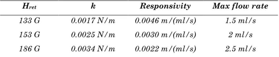
TABLE 3-4SUMMARY OF THE DEVICE PERFORMANCES AS A FUNCTION OF THE RETAINING MAGNETIC FIELD. ... 87

TABLE 3-5 CALIBRATION MODELS OF THE FLOW SENSOR IN DIFFERENT OPERATING CONDITIONS. ... 91

TABLE 3-6 DEVICE SPECIFICATIONS FOR THREE DIFFERENT VALUES OF THE RETAINING MAGNETIC FIELD. ... 91

TABLE 3-7PARAMETER VALUES OF THE DRIVING SYSTEM. ... 104

TABLE 3-8PARAMETER VALUES OF THE SENSING SYSTEM. ... 104

TABLE 4-1CHARACTERISTIC OF ELECTROMAGNETS USED IN THE MATLAB® SIMULATION. ... 117

(26)

TABLE 4-2 OPERATIVE CONDITIONS OF THE ELECTROMAGNET AS FUNCTION OF THE DESIRED CURRENT VALUE. ... 145

TABLE 5-1 GEOMETRIC CHARACTERISTICS OF DIFFERENTIAL TRANSFORMER. ... 156

(27)

Introduction

It is quite common, in the advances on scientific research, to witness how material properties are exploited toward sensing applications in order to realize novel devices with high performances and tunable cha-racteristics.

The synthesis of materials that are not in nature but that are rea-lized in chemical laboratories is often a response to such a requirement. In particular “meta” materials and, in general, those materials made by the aggregation of several components to result into a multi-phase compound, are often very flexible and can provide very interest-ing performance in many different application fields.

Among these, magnetic materials have gained great relevance thanks to the possibility of controlling many of their features via exter-nal magnetic fields but also to the fact that their presence, position or space distribution, is easily detectable by using magnetic sensors.

(28)

In this Thesis an innovative approach to the development of com-plex devices made by multiple sensing parts together with actuators, and an integrated micro-fluidic system are considered.

The basic concept here is the use of new materials, called ferrofluids or magnetic fluids, made by a suspension of magnetic nanoparticles in a carrier fluid; several different devices have been developed and are shown here in order to demonstrate the possibility to use ferrofluids as a core material to realize both the actuating section of a fluidic system and the sensing.

The devices realized have been developed as laboratory prototypes and as proofs of concept of the ideas that have been first conceived, and then mathematical and numerical modeled prior to be designed as expe-rimental devices.

Due to the intrinsic magnetic nature of the ferrofluids, a briefly in-troduction on basic concepts about magnetism is discussed in Chapter 1. A classification of materials in nature according to their magnetic beha-vior is reported, together with some details about the two fundamental source of magnetism: permanent magnets and electromagnets. Finally the main typologies of magnetic sensors commercially available are dis-cussed.

In Chapter 2 the magnetic fluids are presented, together with their applications both in the market and in the research world. The main forces acting on a ferrofluid mass are discussed and modeled.

In Chapter 3 the attention is focused toward sensors realized dur-ing this Ph.D. research activity: a gyroscope, a displace-ment/acceleration sensor, a flow sensor and an inclinometer are

(29)

dis-Introduction 3

cussed, together with their physical model and with the experimental characterization.

In Chapter 4 research results on ferrofluids when used in actuators are presented. Plungers, valves and a position control system for ferrof-luids drop in water have been developed. Two devices are presented: a pump in which a ferrofluid mass is controlled by an array of electro-magnets, and a path tracking system, in which a mass is moved along a pre-defined path by a matrix of electromagnets.

The implementation toward integrated device is nowadays of para-mount importance in the development of novel systems and transduc-ers. The devices presented here has been developed as laboratory proto-type and their scaling toward microsystems is straightforward and has been also addressed during this Ph.D. activity. In Chapter 5 two exam-ples of integrated system in which ferrofluids can be used both in the fluidic part and in the sensing devices are presented. The former struc-ture is a system that can be used for biological measures; in this case ferrofluid is used both in the fluidic part implementing valves and plun-ger, and as magnetic label for biological entities. The latter one represents a multi-sensorial systems, in which ferrofluids are used in order to implement valves and also as inertial mass of the sensors inte-grated in the structure.

(30)

(31)

Chapter 1

T

HE MAGNETISM

1.1. Magnetism in matter

An electron moving around his nucleus constitutes a tiny current loop (because it is a moving charge), having in this way a magnetic moment associated with the orbital motion.

All substances contain electrons, but not all substances are magnet-ic, because in most substances the magnetic moment of one electron in an atom is canceled by that of another electron orbiting in the opposite direction. The net result is that, for most materials, the magnetic effect produced by the orbital motion of the electrons is either zero or very small.

In addition to its orbital magnetic moment, the spin of the electron contributes to its magnetic moment. The magnitude of the angular

(32)

mo-mentum associated with spin is of the same order of magnitude as the angular momentum due to the orbital motion. In non-magnetic atoms, for each electron spinning in one direction, there is another electron spinning in the opposite direction. The atom is said to be in a state of magnetic balance and the total spin magnetic moments is zero. A state of magnetic unbalance exists when there are more electrons spinning in one direction than the opposite direction.

The magnetic properties of an atom increase in direct proportion to the number of electrons that are not compensated. The total magnetic moment of an atom is the vector sum of the orbital and spin magnetic moments.

The nucleus of an atom also has a magnetic moment associated with its constituent protons and neutrons. However, the magnetic mo-ment of a proton or neutron is much smaller than that of an electron (due to their much greater mass) and can usually be neglected.

The magnetic state of a substance is described by the magnetization . The magnitude of this vector is defined as the magnetic moment per unit volume of the substance. The total magnetic field at a point with-in a substance depends both on the applied (external) field and on the magnetization of the substance, in according with the following equa-tion:

(1.1)

where is the field produced by the magnetic substance, is the applied magnetic field and is the permeability of the free space (4π*10-7 H/m).

(33)

The magnetism 7

Introducing the magnetic field strength , the previous equation can be expressed as:

(1.2)

1.2. Classification of magnetic materials

Substances can be classified in three categories depending on their magnetic properties. Paramagnetic and ferromagnetic materials are those made of atoms that have permanent magnetic moments. Diamag-netic materials are those made of atoms that do not have permanent magnetic moments [1], [2].

For paramagnetic and diamagnetic substances, the magnetization vector is proportional to the magnetic field strength . For these sub-stances placed in an external magnetic field, it can be written:

(1.3)

where is a dimensionless factor called the magnetic susceptibility. For paramagnetic substances, is positive and is in the same direc-tion as . For diamagnetic substances, is negative and is opposite to . Substituting Equation 1.3 into Equation 1.2 the following relation-ship is obtained:

(1.4)

where the constant is called the magnetic permeability of the substance and is related to the susceptibility by:

(34)

Substances may be classified in terms of how their magnetic per-meability compares with as follows:

Paramagnetic Diamagnetic

Because is very small for paramagnetic and diamagnetic sub-stances is nearly equal to for these substances. For ferromagnetic substances, however, is typically several thousand times greater than . is not a linear function of for ferromagnetic substances. This is because the value of is not only a characteristic of the ferro-magnetic substance but also depends on the previous state of the sub-stance and on the process underwent when it moved from its previous state to its present one.

Ferromagnetism

A small number of crystalline substances in which the atoms have per-manent magnetic moments exhibit strong magnetic effects called ferro-magnetism.

These substances contain atomic magnetic moments that tend to align parallel to each other even in a weak external magnetic field. Once the moments are aligned, the substance remains magnetized after the external field is removed. This permanent alignment is due to a strong coupling between neighboring moments.

All ferromagnetic materials are made up of microscopic regions called domains, regions within which all magnetic moments are aligned. In an unmagnetized sample, the domains are randomly oriented so that the net magnetic moment is zero, as shown in Figure 1-1a. When the

(35)

The magnetism 9

sample is placed in an external magnetic field, the magnetic moments of the atoms tend to align with the field, which results in a magnetized sample, as in Figure 1-1b.

a) b)

Figure 1-1 a) Random orientation of atomic magnetic moments in an unmagne-tized substance. b) When an external field is applied, the atomic magnetic

moments tend to align with the field, giving the sample a net magnetization vector .

When the external field is removed, the sample may retain a net magnetization in the direction of the original field. At ordinary temper-atures, thermal agitation is not sufficient to disrupt this preferred orientation of magnetic moments.

The described dipole ordering usually does not extend over the en-tire volume of a sample. Rather, a sample of magnetic material is split up into domains in which all dipoles are ordered along a preferential di-rection (see Figure 1-2). This didi-rection changes from domain to domain, and it is for this reason that bulk magnetic materials may be unmagne-tized, even though they are magnetized on the length scale of the do-mains.

(36)

In an external magnetic field, the magnetization directions of the domains are forced to align with the field, or domains with favorable magnetization direction will grow at the cost of domains with unfavora-ble directions. Both mechanisms increase the net magnetization of the bulk material. At infinite magnetic field strength, all dipoles are aligned with the field, and the system has reached its saturation magnetization.

Figure 1-2 In bulk ferromagnetic materials dipole alignment is split up into domains.

After the field is removed, the magnetization tends to relax into its original state with randomly oriented domains. However, in order to reach that equilibrium state, the system may have to pass unfavorable states that can keep it from actually reaching equilibrium. Materials for which the relaxation to the unmagnetized state is prevented, are called “hard” magnetic, as opposed to “soft” magnetic materials, which demag-netize quickly upon removal of the external field or application of a small field opposing the magnetization.

The magnetic properties of ferroelectric materials can be described by plotting a hysteresis loop for the magnetization, , of the material as a function of the applied magnetic field, . Its shape and size depend on

(37)

The magnetism 11

the properties of the ferromagnetic substance and on the strength of the maximum applied field.

The hysteresis loop for hard ferromagnetic materials is characte-rized by a large remanent magnetization. Soft ferromagnetic materials have a very narrow hysteresis loop and a small remanent magnetiza-tion, as shown in Figure 1-3.

Figure 1-3 Magnetic hysteresis loops for Soft and Hard materials

By heating the material above a critical temperature (the Curie temperature), the thermal agitation is great enough to cause a random orientation of the moments: the substance loses its ferromagnetic prop-erties and becomes paramagnetic.

Paramagnetism

Paramagnetic substances have a small but positive magnetic sus-ceptibility resulting from the presence of atoms (or ions) that have per-manent magnetic moments. These moments interact only weakly with each other and are randomly oriented in the absence of an external magnetic field.

(38)

When a paramagnetic substance is placed in an external magnetic field, its atomic moments tend to line up with the field. However, this alignment process must compete with thermal motion, which tends to randomize the magnetic moment orientations. The magnetization of a paramagnetic substance is proportional to the applied magnetic field and inversely proportional to the absolute temperature, as expressed in the Equation 1.6:

(1.6)

This relationship is known as Curie’s law and the constant C is called Curie’s constant; is the absolute temperature measured in Kel-vin.

Diamagnetism

When an external magnetic field is applied to a diamagnetic substance, a weak magnetic moment is induced in the direction opposite the ap-plied field. This causes diamagnetic substances to be weakly repelled by a magnet.

Although diamagnetism is present in all matter, its effects are much smaller than those of paramagnetism or ferromagnetism, and are evident only when those other effects do not exist.

Antiferromagnetism

In materials that exhibit antiferromagnetism, the magnetic moments of atoms or molecules align in a regular pattern with neighboring spins pointing in opposite directions. This spontaneous antiparallel coupling of atomic magnets may exist at sufficiently low temperatures: in fact, it

(39)

The magnetism 13

is disrupted by heating and disappears entirely above a certain temper-ature, called the Néel tempertemper-ature, characteristic of each antiferromag-netic material. Some antiferromagantiferromag-netic materials have Néel tempera-tures at, or even several hundred degrees above, the room temperature, but usually these temperatures are lower. Above the Néel temperature, the material is typically paramagnetic.

Antiferromagnetic solids exhibit special behaviour in an applied magnetic field depending upon the temperature. At very low tempera-tures, the solid exhibits no response to the external field, because the antiparallel ordering of atomic magnets is rigidly maintained. At higher temperatures, some atoms break free of the orderly arrangement and align with the external field. This alignment and the weak magnetism it produces in the solid reach their peak at the Néel temperature. Above this temperature, thermal agitation progressively prevents alignment of the atoms with the magnetic field, so that the weak magnetism pro-duced in the solid by the alignment of its atoms continuously decreases as temperature is increased.

Ferrimagnetism

The ferrimagnetism is a type of magnetism in which the magnetic mo-ments of neighboring ions tend to align nonparallel, usually antiparal-lel, to each other, as in the antiferromagnetic materials; but unlike the antiferromagnetic, in the ferromagnetic substances the moments are of different magnitudes, so there is an appreciable resultant magnetiza-tion.

The materials are less magnetic than ferromagnets. Ferrimagnetic materials are like ferromagnets in that they hold a spontaneous

(40)

magne-tization below the Curie temperature, and show no magnetic order (are paramagnetic) above this temperature, but the spontaneous alignment is restored upon cooling below the Curie point. However, there is some-times a temperature below the Curie temperature at which the number of ions aligned parallel is equal to the number of ions aligned antiparal-lel, resulting in a net magnetic moment of zero; this is called the magne-tization compensation point.

Ferrimagnetism occurs mainly in magnetic oxides known as fer-rites.

In Figure 1-4 schematic pictures of the magnetic moments behavior in the different kind of materials above described, are reported.

Figure 1-4 Types of magnetism: paramagnetism, ferromagnetism, antiferro-magnetism and ferriantiferro-magnetism.

In Table 1-1 magnetic response of various materials is compared with their susceptibility and permeability values.

(41)

The magnetism 15

Table 1-1 Comparison between different kind of magnetic materials as function of permeability and susceptibility

Diamagnetism Paramagnetism Ferro-Ferrimagnetism Susceptibility <0 ≥0 >>0 Relative

permea-bility <1 ≥1 >>1

1.3. Sources of magnetic field

A magnetic field can be arisen from two sources:

 Electric currents or more generally, moving electric charges create magnetic fields. Electromagnets exploit such a physical principle.

 Hard ferromagnetic materials can be magnetized by a strong magnetic field, becoming themselves sources of magnetic field. Permanent magnets or electromagnets can produce the same mag-netic field.

Electromagnets

An electric current flowing in a wire creates a magnetic field around the wire, as expressed by the Biot-Savart law, reported in Equation 1.7.

(1.7)

where is the current, is a vector, whose magnitude is the length of the differential element of the wire, and whose direction is the direc-tion of convendirec-tional current, and is the displacement unit vector in the

(42)

direction pointing from the wire element towards the point at which the field is being computed.

To concentrate the magnetic field, the electromagnet wire is wound into a coil, with many turns of wire lying side by side. The magnetic field of all the turns of wire passes through the center of the coil, creat-ing a strong magnetic field there.

Much stronger magnetic fields can be produced if a "core" of ferro-magnetic material, such as soft iron, is placed inside the coil. The fer-romagnetic core increases the magnetic field to thousands of times the strength of the field of the coil alone, due to the high magnetic permea-bility of the ferromagnetic material.

The main advantage of an electromagnet over a permanent magnet is that the magnetic field can be rapidly manipulated over a wide range by controlling the amount of electric current. The poles of an electro-magnet can even be reversed by reversing the flow of electricity. How-ever, a continuous supply of electrical energy is required to maintain the field.

The magnetic field produced by an electromagnet driven with a cur-rent can be expressed as:

(1.8)

where is the turn number, L is the length of the electromagnet and R is the radius of the electromagnet.

(43)

The magnetism 17

The qualitative magnetic field behavior is shown in Figure 1-5: the maximum value is at the electromagnet center ( ).

Figure 1-5 Behavior of the magnetic field produced by an electromagnet cen-tered in with a radius .

Permanent magnets

A permanent magnet is an object made of ferromagnetic material that is magnetized in one direction by a very strong field and that creates its own persistent magnetic field; due to the ferromagnetic properties of the used material, a magnet doesn’t relax back to zero magnetization when the imposed magnetizing field is removed. To demagnetize the magnet it has to be put inside a strong field in the opposite direction of that one used to magnetize it.

A good permanent magnet should produce an high magnetic field with a low mass, and should be stable against the influences which would demagnetize it.

Permanent magnets have several advantages over conventional electromagnets. The fundamental advantage is that they can provide a

-0.040 -0.02 0 0.02 0.04 1 2 3 4 5 6x 10 -3 x [m] Mag net ic fi el d [T ]

(44)

relatively strong magnetic field over an extended spatial region for an indefinite period of time with no expenditure of energy.

Another advantage of permanent magnets is that they can be fabri-cated with a wide range of structural properties, geometric shapes, and magnetization patterns.

Permanent magnets have an additional advantage over electro-magnets in that their performance scales well with size. Specifically, if we change a linear dimensions L of an electromagnet, while keeping the field strength at all the rescaled observation points fixed, the current density must be adjusted by a factor of 1/L. By comparison, if we change the linear dimensions of a permanent magnet, the field strength at all the rescaled observation points remains constant (assuming the magne-tization is constant).

Thus, there will be a dimension below which a permanent magnet will be the only viable field source.

The magnetic field produced by a cylindrical magnet of magnetiza-tion can be expressed as:

(1.9)

where L is the length of the magnet and R is the radius of the mag-net. Equation 1.9 is valid only for .

(45)

The magnetism 19

Figure 1-6 Behavior of the magnetic field produced by a permanent magnet centered in and with a radius .

1.4. Magnetic sensors

The term magnetic sensor refers to various kinds of sensor based to dif-ferent working principles and used to sense difdif-ferent physical entities.

However, all the magnetic sensors are based on a response to a magnetic quantity: such a response can be directly or indirectly related to the quantity to measure.

Magnetic field sensors are used to measure the amplitude of a mag-netic field acting in the area surrounding the device or a field perturba-tion due to the presence of some magnetic materials. Their output is di-rectly connected with the magnetic field amplitude to detect.

If the target to detect is the amount of a magnetic material, sensors of magnetic materials can be utilized; the amplitude of an external ap-plied magnetic field is modified by the magnetic material, and the change depends on the material amount. The output of this kind of

de--0.010 0 0.01 0.02 0.03 0.04 0.05 0.1 0.15 0.2 0.25 0.3 x [m] Mag net ic fi el d [T ]

(46)

vices is directly connected with the amount of magnetic material to detect.

The third class of sensors exploits the relationship between an ex-ternal magnetic field or a magnetic force and a physical inex-ternal entity of the sensor; the target is not a magnetic quantity, but it is related with it; in this way, the output can be indirectly obtained through this relationship.

Magnetic field sensors

Magnetic field strength is measured using a variety of different technol-ogies. Each technique has unique properties that make it more suitable for particular applications. These applications can range from simply sensing the presence or change in the field to the precise measurements of a magnetic field’s scalar and vector properties.

Magnetic field sensors can be divided into vector component and scalar magnitude types. The vector types can be further divided into sensors that are used to measure low fields (<1 mT) and high fields (>1 mT). Instruments that measure low fields are commonly called magne-tometers. High-field instruments are usually called gaussmeters. A schematization of the different kind of sensor is reported in Figure 1-7.

The induction coil and fluxgate magnetometers are the most widely used vector measuring instruments. They are rugged, reliable, and rela-tively less expensive than the other low-field vector measuring instru-ments.

The fiber optic magnetometer is the most recently developed low-field instrument. Although it currently has about the same sensitivity as a fluxgate magnetometer, its potential for better performance is

(47)

The magnetism 21

large. The optical fiber magnetometer has not yet left the laboratory, but work on making it more rugged and field worthy is under way.

The superconducting quantum interference device (SQUID) magne-tometers are the most sensitive of all magnetic field measuring instru-ments. These sensors operate at temperatures near absolute zero and require special thermal control systems. This makes the SQUID based magnetometer more expensive, less rugged, and less reliable.

The Hall effect device is the oldest and most common high-field vec-tor sensor used in gaussmeters. It is especially useful for measuring ex-tremely high fields (>1 T).

The magnetoresistive sensors cover the middle ground between the low- and high-field sensors. Anisotropic magnetoresistors (AMR) are currently being used in many applications, including magnetometers.

The recent discovery of the giant magnetoresistive (GMR) effect, with its tenfold improvement in sensitivity, promises to be a good com-petitor for the traditional fluxgate magnetometer in medium-sensitivity applications.

The proton (nuclear) precession magnetometer is the most popular instrument for measuring the scalar magnetic field strength. Its major applications are in geological exploration and aerial mapping of the geomagnetic field. Since its operating principle is based on fundamental atomic constants, it is also used as the primary standard for calibrating magnetometers. The proton precession magnetometer has a very low sampling rate, on the order of 1 to 3 samples per second, so it cannot measure fast changes in the magnetic field.

(48)

The optically pumped magnetometer operates at a higher sampling rate and is capable of higher sensitivities than the proton precession magnetometer, but it is more expensive and not as rugged and reliable.

Figure 1-7 Magnetic field sensors are divided into two categories based on their field strengths and measurement range: magnetometers measure low fields

and gaussmeters measure high fields.

Sensors of magnetic quantities

Magnetic fields are typically conceptualized with so-called “flux lines” or “lines of force.” When such flux lines encounter a magnetic material, an interaction takes place and consequently the number of flux lines is ei-ther increased or decreased. The original magnetic field density ei- there-fore becomes amplified or diminished as a result of the interaction.

(49)

The magnetism 23

The amount of the magnetic field change depends on the quantity of the magnetic material placed in the area in which the magnetic field is acting. Measuring the magnetic field change it is possible to obtain the magnetic material amount; this kind of sensors allows to detect also the presence of a single bead of a magnetic material, for example, if the di-mension of the active part of the sensor is comparable with the dimen-sion of the bead.

Usually superparamagnetic beads are used due to their property to not retain a magnetization imposed through an external magnetic field when the field is removed.

Several kinds of sensor were developed and used to sense an amount of magnetic beads. Usually they are based on a differential con-figuration: the sensor compares the output due only to the field with the output due to the field increased by the beads. The sensor output is then related with the beads quantity.

Sensors exploiting magnetic forces as working principle

This class of sensors is based on a relationship between the magnetic force (or the magnetic field) and the entity to detect; the output of the sensor is then indirectly related with the target entity. The most com-mon sensor is the LVDT (Linear Variable Differential Transformer).

It is based on the variation in mutual inductance between a prima-ry winding and each of two secondaprima-ry windings when a ferromagnetic core moves along its inside, dragged by a nonferromagnetic rod linked to the moving part to sense. When the primary winding is supplied by an ac voltage, in the center position the voltages induced in each secondary winding are equal and the output voltage is zero because it is

(50)

differen-tial. When the core moves from that position, one of the two secondary voltages increases and the other decreases of the same amount, and the output is different from zero. The secondary coil voltage changes with the position of the core because the core modifies the field produced by the primary winding; such a modification changes the auto inductance value of the secondary coil, that it is reported on the output voltage. Such a sensor exploits the relationship between the magnetic core and the output voltage in order to detect the core position. The output then is indirectly related with the target represents by the core position.

(51)

Chapter 2

F

ERROFLUIDS AND THEIR APPLICATIONS

2.1. Ferrofluids

Ferrofluids (also called magnetic fluids or magnetic nanofluids) are a special category of nanomaterials which exhibit simultaneously liquid and superparamagnetic properties.

Due to the fact that no natural liquids offer these features, the starting point of the field of magnetic fluid research can be found in a work of Resler and Rosensweig [3]. Such a work showed that a liquid material with controllable magnetic properties can be used in many de-velopment possibilities. After that, strong efforts have been undertaken to synthesize a system enabling the mentioned magnetic control. Sus-pensions of magnetic nanoparticles in appropriate carrier liquids are a sufficient realization of such a new class of smart materials. Although

(52)

non-stable suspensions have been produced much earlier, the first sta-ble synthesis of a ferroﬂuid was reported in the pioneering work by Pa-pell [4], in 1965. The development of these suspensions – called ferroflu-ids – proved the high potential of the new research field.

In the past 40 years since the first synthesis of a ferrofluid has been reported, a large number of technical applications was realized. Review-ing the proposed applications it can be noticed that those which have been successful on the market are characterized by two basic traits. The first one consists in the use of the magnetic field only to exert a force in order to fix the mass position. The second one is that all technical appli-cations were realized mainly in the field of mechanical engineering.

Today the perspectives of ferrofluid research are much broader. The force enters directly into the Navier–Stokes equation and can thus be utilized to control and drive flows in the fluid, not only to provide a force positioning the ferrofluid. Taking into account that strength and direc-tion of magnetic fields and field gradients can be tailored for a specific need, one can imagine the variety of arising possibilities. Furthermore not only the flow of magnetic suspensions can be changed by magnetic fields but also their thermophysical properties –in particular the rheo-logical behavior– change significantly in the presence of magnetic fields. In fact, modifying the magnetic field intensity, is possible to change pa-rameters as density and viscosity.

Modern ferrofluids are colloidal magnetic fluids. A colloid is a sus-pension of finely divided nanoparticles [5], such as Fe3O4, γ-Fe2O3,

CoFe2O4, Co, Fe or Fe-C, in a continuous medium. They are composed

by small particles of solids, magnetic, single-domain particles coated with a molecular layer and a dispersant (surfactant), and suspended in

(53)

Ferrofluids and their applications 27

a liquid carrier. The colloidal ferrofluid must be synthesized, because it is not found in nature. The three primary constituents of these magnetic liquids are:

 The liquid carrier in which the particles are suspended. Ferrof-luids can be water- or oil-based [6].

 The suspended superparamagnetic particles are made from materials such as iron oxide, and have a diameter of the order of 10-20 nm. The small size is necessary to maintain stability of the colloidal suspension; particles significantly larger than this would precipitate.

 The surfactant coats the ferrofluid particles to help maintain the consistency of the colloidal suspension. The surfactant pre-vents interactions and agglomeration of particles caused by Van der Waals forces [7].

A scheme of ferrofluid particles is reported in Figure 2-1.

Figure 2-1 Schematic of ferrofluid particles, with highlighted the magnetic core and the surfactant.

(54)

The particles are sufficiently small so that the ferrofluid retains its liquid characteristics even in the presence of a magnetic field, and sub-stantial magnetic forces can be induced which results in fluid motion. The magnetic liquid can then be considered as an ultrafine particle sys-tem with interparticle spacing large enough to approximate the par-ticles as non-interacting.

The size of the particles makes the difference between the two types of fluids which depend on the applied magnetic field: ferrofluids and magneto-rheological fluids. Magneto-rheological fluids are stable sus-pensions of magnetically polarisable micron-sized particles suspended in a carrier fluid. These fluids vary their viscosity with the applied magnetic field and can solidify in the presence of a sufficient magnetic field. In comparison, ferrofluids retain liquid flowability even in the most intense applied magnetic fields. Ferrofluids are usually described as magnetically soft material, which means that the magnetism vector follows the applied field without hysteresis, and a small applied field is required to produce saturation. Instead an high magnetization strength implies high magnetic pressure exerted by the fluid. The latter property is strategic for the implementation of transducers adopting ferrofluids as functional or inertial masses. Ferrofluids present a high magnetiza-tion saturamagnetiza-tion ranges from 200 to 900 G, approximately with no rema-nence and, as a liquid, they can be easily moved through microchannels, and perfectly adapt to any geometry.

When a ferrofluid mass is subjected to an external magnetic field, hits flat surface could become unstable and shows a behavior called Ro-sensweig effect. At a certain intensity of the field, peaks appear at the fluid surface, which typically form a static hexagonal pattern at the

(55)

fi-Ferrofluids and their applications 29

nal stage of the pattern forming process. Such a typical response is shown in Figure 2-2.

Figure 2-2 Examples of ferrofluids subjected to magnetic fields.

Magnetic fluids show also interesting patterns, coming from ferro-hydrodynamic instabilities, such as lines, labyrinths and various struc-tures which could be exploited to produce actuation. In [8] authors im-pose, on a magnetic fluid preliminarily separated into concentrated and dilute phases, an alternating electric field of opportune amplitude and frequency, and a superimposed orthogonal constant magnetic field. The imposed field causes the formation of a labyrinth structure, as reported in Figure 2-3.

Figure 2-3 Structural lattices formed in a thin layer of the magnetic fluid ex-posed to an alternating electric field at different frequencies: a) 2 and

(56)

A magnetic field applied to a ferrofluid volume exerts a magnetic force which causes the alignment of the ferrofluid particles in the direc-tion of the field. In the absence of external magnetic field the ferrofluid maintains its liquid status while under the magnetization produced by a strong magnetic field the ferrofluid modifies its physical properties, as viscosity and density, and moves to a more compliant position.

2.2. Applications of ferrofluids

Fluids which can be controlled and manipulated by external magnetic fields of moderate strength are a challenging subject for scientists inter-ested in fluid movement or in application engineering.

When the magnetic influence exerted by an external magnetic field becomes strong enough to compete with gravitational forces, it is possi-ble a complete control of the magnetic fluid mass movement and of its physical properties.

The possibility of using different types of coils (controlling and switching electronically the current) and permanent magnets allows for a wide range of magnetic field intensity, so the technical application of such a materials is very large and various.

The research field of magnetic fluids is a multi-disciplinary area: chemists study their synthesis and produce the ferroﬂuids, physicists study their physical properties and propose theories which explain them, engineers study their applicability and use them in technological products, biologists and physicians study their biomedical possibilities and use them in medicine and in research on the biological area.

(57)

Ferrofluids and their applications 31

With modern advances in understanding nanoscale systems, cur-rent research focuses on synthesis, characterization, and functionaliza-tion of nanoparticles with magnetic and surface properties tailored for application as micro-nanoelectromechanical sensors, actuators, in mi-cro-nanofluidic devices, as nanobiosensors, and in biomedical applica-tions.

Commercial applications of ferrofluids

Ferrofluids allow applications in each of its constituent disciplines of chemistry, fluid mechanics, and magnetism. An important property of concentrate ferrofluids is that they are strongly attracted by permanent magnets, while their liquid nature is preserved. The attraction can be strong enough to overcame the gravity force. Many commercial applica-tions of ferrofluids are based on this properties. Sealing for several in-dustrial processes, loudspeakers, inertial dampers, angular position sensors, computer disk drives are examples of applications where this kind of materials has been widely adopted [9],[10].

For example, in hard disks they are used to form liquid seals around the spinning drive shafts. The rotating shaft is surrounded by magnets. A small amount of ferrofluid, placed in the gap between the magnet and the shaft, will be held in place by its attraction to the mag-net. The fluid of magnetic particles forms a barrier which prevents de-bris from entering the interior of the hard drive.

In loudspeakers ferrofluids are used to remove heat from the voice coil, and to passively damp the movement of the cone. They reside in what would normally be the air gap around the voice coil, held in place by the speaker's magnet. Since ferrofluids are paramagnetic, they obey

(58)

Curie's law, thus become less magnetic at higher temperatures. A strong magnet placed near the voice coil (which produces heat) will at-tract cold ferrofluid more than hot ferrofluid thus forcing the heated fer-rofluid away from the electric voice coil and toward a heat sink.

Biomedical applications of ferrofluids

Ferrofluids are nowadays assuming a fundamental role in biomedical applications for diagnostic and therapy [11]. These materials find inter-esting applications in magnetic bio-assay tasks, such as magnetic sepa-ration, drug delivery, hyperthermia treatments, magnetic resonance imaging (MRI) and magnetic labelling. In fact, due to the different and controllable sizes of their particles (from few nanometers up to micro-meters), they can interact with the biological entity of interest like a cell (10–100 µm), a virus (20–450 nm), a protein (5–50 nm) or a gene (2 nm wide and 10–100 nm long), thus offering attractive possibilities to de-velop efficient solutions in the bio-medical field. Examples of such tech-niques can be found in [12], [13], [14].

Magnetic particles coated with biocompatible molecules act as markers to identify bio-entities. The main advantage of this form of la-belling as compared to other techniques is related to the simple mechan-isms to identify, to localize and to transport magnetic labelled entities. Actually, all these mechanisms are based on the use of magnetic fields which are also intrinsically penetrable into human tissue. Magnetic la-belling is used for both entities localization and separation.

Magnetic separation is a two-step process: the first step consists in labelling the molecules to be detected with magnetic beads; this is ob-tained by coating the magnetic particle surface with specific

(59)

biocom-Ferrofluids and their applications 33

patible molecules to allow the binding with the target entity. The second step consists in separating the labelled molecules from their native by blocking the magnetic particles via a magnetic field. The same principle is used to remove unwanted biomaterials from a fluid, capturing the magnetic particles with a magnet or with a magnetic field gradient and letting flow the remaining fluid.

A promising use of magnetic fluid in biomedicine is drug delivery which has peculiar advantages as compared to traditional techniques. In fact, today therapeutic drugs act on the entire body (e.g. by attacking both tumour tissue and healthy ones) while with selective drug delivery only specific locations of the body are attacked. This approach allows to reduce the required drug dosage, to increase drugs specificity as well as prolonging the use of these effective agents. The magnetic particles bounded with the drugs are injected through the circulatory system while an external high-gradient magnetic field is used to deliver tasks.

Another possibility for tissues (e.g. cancer) treatments is the hyper-thermia. Such technique consists of embedding magnetic particles into the target tissue and applying a suitable magnetic field to cause parti-cles heating. This heat radiates into the surrounding tumour tissue thus to destroy, after a specific length of time, the cancer cells. While other hyperthermia methods produces unacceptable heating of human healthy tissue, magnetic hyperthermia overcome these drawbacks by a selective heating of target cells.

MRI is a non-invasive technique that allows the characterization of morphology and physiology in vivo through the use of magnetic scan-ning. The human body is mainly composed of water molecules contain-ing protons which under powerful magnetic field align with the

(60)

direc-tion of the field. A second radio frequency electromagnetic field is then briefly turned on causing the protons to absorb some of its energy. When this field is turned off the protons release this energy at a radio frequency which can be detected by a scanner. Relaxation times of pro-tons in diseased tissue, such as tumours, are different than in healthy tissue and this information is used for the sake of inspection. Magnetic nanoparticles can be conveniently used in MRI techniques as contrast agent.

Transducers based on the use of ferrofluids

Practical interest in magnetic fluids derives from the possibility to im-plement valuable and efficient conversion of elastic energy into mechan-ical energy [15].

The use of magnetic fluids in transducers is now widely diffused due to valuable properties of these fluids compared to traditional mate-rials [16]. Actually, fast response, shock resistance and their intrinsic feature to be shapeless allow to develop suitable sensors and actuators.

The idea of using ferrofluids as the active mass in inertial sensors offers the opportunity to control the device specifications by manipulat-ing the ferrofluid core properties (such as viscosity, volume, etc.) via electric signals. Moreover, the absence of mechanical moving parts and solid-inertial masses provide high reliability and robustness against mechanical shocks.

Actually in case of traditional inertial sensors exploiting a solid mass a mechanical shock could compromise the device functionality while the use of ferrofluid allows for recovering the system functionality by re-aggregation.