DYNAMIC MANAGEMENT MODEL FOR
OFFHIRE MOVEMENTS OF A CARRIER FLEET
M. de Falco a, M. E. Nenni b, M. M. Schiraldi c a) Università di Lecce, Lecce, Italy
tel. +39.081.7682333 - defalco@unina. it b) Università di Napoli “Federico II”, Naples, Italy
tel. +39.06.7259. 7179 - nenni@uniroma2. it c) Università di Roma “Tor Vergata”, Rome, Italy
tel. +39.06.7259.7179 - schiraldi@ing. uniroma2. it
KEYWORDS
Dead-head movements, off-hire carriers, transportation, route optimization, waiting areas, deviation points.
1. ABSTRACT
This paper presents an innovative dynamic route management model for direct on-demand transportation services. In these scenarios, a carrier is hired for a transportation service from an origin to a destination point and then released. Subsequently, being in the off-hire condition, the carrier can wait in the destination point or move towards another loading dock. The aim of the approach is to identify the best route and the optimal waiting strategy of the carrier while in the off-hire condition, minimizing the dead-head movement costs and maximizing the expected profit originating from the forecasted demand. This model has been tested in the industry of the oil tankers fleet.
So far this problem has been partially fronted with models which are focused on the evaluation of each loading dock profitability, lacking however to consider the opportunity of a continuous-moves routing in the off-hire condition.
This analysis defines instead a dynamic strategy which estimates the future demand and is continuously updated by the other carriers movements and by the variation in the scenario. A set of Deviation
Points and Waiting Areas are identified respectively as alternatives for
the carrier off-hire movements and as areas in which the carrier has the possibility to stop and wait for a new order. These points are determined on a geographical map on behalf of statistical and economical considerations. Time constraints are also considered, especially in terms of Time Windows in which the carrier has to react to the demand and to reach the origin of the order.
2. OFF-HIRE CARRIERS AND DEAD-HEAD MOVEMENTS
In direct on-demand transportation services, a carrier is hired for a transportation service from a Pickup Point (PP) to a Delivery Point (DP) without intermediate stops (Powell, 1988). The relevant information concerning the customer order are the PP and the DP, besides, of course, the price customers will pay for the service and the
Time Window (TW) that indicates the period in which the carrier is
asked to start the transportation service from the PP. The various companies which manage carrier fleets try to coordinate their carriers movement in order to match the demand and to catch the most profitable orders. The customer order distribution is uncertain under both the geographical and the economical issues, which means that it is
not possible to know in advance where the next order will be released (which is going to be the next PP) neither which kind of transportation service will be required (how much money will be offered and which will be the DP). As a consequence, the possibility to plan the carrier movements in advance is minimal (Powell, Sheffy, Nickerson, 1987). The fleet management continuously collects information on the position of his carriers to decide whether to accept a certain order originating from a certain PP or not. If the order is considered to be adequately profitable then it is accepted and the fleet management gives instruction to the carrier to reach the PP (which is said to be the origin or source of the order) inside the TW. Once the carrier has performed the service and reached the DP, it passes in the off-hire condition and instead of representing a profit center for the company it represents a cost center. The optimal condition would be that the carrier could rapidly find another transportation order originating from that DP but of course this does not always happen; thus, the off-hire carrier must choose between remaining in its position or moving towards another potential PP
(dead-head movement) which will be chosen among the most probable
sources of other orders. Obviously the carrier bears a higher costs when it moves than waiting; besides the difficulty of coordinating all the fleet carriers and the competitors carriers movements, the historical data significance is generally low: high-demand zones can rapidly turn to low-demand zones and vice versa in dependence of exogenous influences and it is not possible to accurately predict if a certain PP will be the source of an order in a given period of time. In this essential scenario we already encounter some substantial difficulties. First of all, the order profitability evaluation is critical; despite an apparently high
profitability indeed, the asked transportation service can lead the carrier in a low-demand zone thus forcing the carrier to long, costly and time-consuming dead-head movements to reach the next order source. Thus appears fundamental to follow a correct stop-or-move strategy (and, in case, to chose the best route) once in the off-hire condition, which we will put at center of our effort.
According to the literature, the order profitability can be evaluated in two ways: with the direct method only the revenues and the costs of the PP-DP travel are considered, obviously in dependence by the transportation service duration. In the tank-oil industry the World-Scale
Rate is used to determine the profitability of a direct on-demand
transportation service through the comparison of a direct profitability
index with the daily profitability of a time-charter hire. On the contrary,
with the indirect method, the costs and the time consumption relative to the previous dead-head movement are considered. The choice of attributing the costs of each dead-head movement to the following order is the most commonly used practice. However both of these methods, though are useful to determine a graded list for the various contract alternatives, fail when they are used to determine an effective movement strategy, because the consequences of the acceptance of a specific order are not considered. In the past, few authors have focused the research on the role of the dead-head movements costs in the direct on-demand transportation services (Savelsbergh, 1995); moreover, real-time route optimization was not exploited due to the lack of adequate computing tools. Nowadays this trend has changed thanks to the development of technologies which increase elaboration potentialities and allow carriers tracking; only the implementation of strategies which
are based on continuous system reconfiguration with real-time data collection can grant significant competitive advantage to transportation companies (Powell, Odoni, Jaillet, 1994).
One of the few model which analyzes the problem of the evaluation of order profitability including dead-head costs is the Dynamic Vehicle Allocation Problem (DVA) described by Powell, Sheffy and Nickerson (1988): the DVA is a stochastic model which belongs to the Dynamic Fleet Management model class; it aims to maximize the profit through optimal choices of acceptance/refusal of the orders and through the minimization of the dead-head movement costs. In the DVA model the profitability of each contract is evaluated in dependence of its delivery point indeed. However, the DVA applications suffer from some restrictions, specifically:
- its time-interval aggregation can lead to non-optimal decisions; - the profitability estimation does not consider the short-term
variability of the market;
- the model gives only few indications regarding the optimal routes of off-hire carriers and only suggests to move towards the most probable source of an order;
- the model does not consider the opportunity of a sequence of dead-head movements.
The best route, indeed, may be composed by a succession of movements and stops by which the probability to catch a profitable order (that means: the expected value of the orders that may originates by various PP) is maximized, though the traveled distance is slightly increased in comparison with a straight route. The profitability maximization reached through the analyses of a complex route which
dynamically varies every time unit and in which several PP are passed by in a succession of dead-head movement, is the aim of this paper.
3. WAITING AREAS AND DEVIATION POINTS
Two are the informations which characterize the order as far as the carrier movement timing is concerned: the moment in which the order is released by the customer and the moment in which the TW ends; the difference ∆T between this two parameters represents the available time for the carrier in order to reach the PP. Usually this time interval is constant and fixed, dependent on the operative environment. Furthermore, we will make the hypothesis that the speed of the vectors is constant (vm). This means that, in absence of geographical constraints, which may restrict the carrier movements, to accept an order originating from a certain PP, the carrier must be inside the circle with radius vm⋅∆T and center on the PP. This area is defined Service
Area (SA) of the PP. It is clear how a carrier does not need to reach the
PP in order to be able to catch the potential orders coming from that PP, but it is sufficient to enter in its SA. When two or more SA are relatively extended and the PP relatively near, the SA intersect and an overlap area is created. The overlap area is defined Waiting Area (WA). It is equally clear that in the WA the probability to meet an order is higher because the carrier can rely on the orders originating from more than one PP; this means that each WA is the best area for the carrier to wait for any order originating in any of the PP from which the WA is formed. In many cases as well as in the case we have tested the model, the WA can be significantly large. In our approach, inside each WA is identified a Deviation Point (DP), that means a geographical
point that the carrier must reach before choosing whether to wait or to proceed towards a new WA. By definition, the number of DPs is smaller than the number of PPs; the shift of the focus from the PPs to the DPs would result in the simplification of any traditional algorithm for the optimization of complex routes. The determination of a unique DP inside each WA is important because in this way the crossing time of each WA become fixed (the carrier remains in the WA for a precise interval of time) and, moreover, the DP is chosen in order to place the carrier in an optimal position for the continuation of the journey. For these reasons the position of the DP inside each WA in not fixed a
priori but changes with the route that the carrier is following. To sum
up, a route can be generally intended as a sequence of movements between DP. In order to identify which DP a carrier should pass through we must first introduce a method to evaluate the profitability of being in a WA.
4. EVALUATION OF THE ROUTE PROFITABILITY
The profitability of being inside a certain WA can mainly depends on two factors:
1) the probability to catch an order which is released from one of the PPs from which the WA is generated;
2) the average revenues coming from that order (the revenues coming from the orders released from a specific PP are not all the same). Moreover, the first factor can be related to three elements:
a) the time spent by the carrier inside the WA;
b) the moment in which the off-hire carrier enters in the WA; c) the presence of other off-hire carrier inside the WA.
Indeed, it is true that the probability that an order is released from a PP changes over time, in example among the day of the week or among the hours of the day. Moreover, if an order is released form a certain PP and other carriers are in the off-hire condition in its SA, a criterion must be used to identify the priority of each carrier to carry out the service (the criterion will be based on cooperative or competitive principles depending on the fact that the carriers belong to the same fleet or not). It is possible to obtain some informations through the analysis of PPs historical data. Knowing the frequency distribution of the orders ( i.e., assuming the Poisson distribution) we can determine the probability Pi*(k,s) that exactly (k) orders are released from a certain PP (i) up to a certain time (s). From here it is easy to obtain the probability Pi(k, s) that the PP (i) will release at least (k) orders up to time (s), which is an important information for our purposes, through:
( )
∑
−( )
= − = k 1 0 j * i i k,s 1 P j,s PIn this expression it would be easy to include eventually another parameter which can represent the probability to catch the order due to presence of competitor carriers in the SA of the PP.
Meanwhile, in order to determine the average revenues coming from the orders of one specific PP we can use the end-effect analysis; for an exhaustive description of the end-effects we refer to the DVA model (Powell, Sheffy, Nickerson, 1988): the average revenues Ri(s) being the carrier in the SA of the PP (i) at time (s) is described by:
Ri (s) =
∑
= N n 1 qi n⋅ [π i j + ej(s’)]where the following data are estimated from historical time series analysis:
- qij = on-hire travels percentage among all the travels form the PP (i) to the PP (j);
- πij = average profit of the travel from (i) to (j), that means average revenues of the order minus the average costs for the movement from (i) to (j);
- tm(i, j) = average duration of the travel from (i) to (j);
- ej(s’) = end-effect of the PP (j) in the moment (s’) = [s +tm(i,j)]. With the last term we try to estimate the future profits coming from being the carrier in the PP (j) in time (s’).
The determination of the expected revenues is then carried out multiplying the average revenue of the order with the probability of catching the order itself, that means:
Ei PP
(k, s) = Ri (s) ⋅pi (k, s)
In a similar way, if we want to determine the expected revenues Ei(k,s)=EiWA(k,s) related to a WA instead of those EiPP(k,s) related to a PP we can have: Ei(k, s) = PA(k,s) RA(1,s) +
∑
= k i 0 { [PA * (i,s) PB(k-i,s)] RA(1,s) } Where the WA is originated by two SA respectively of the PP (A) and PP (B) and we have sorted (A) and (B) so that EA(k,s) ≥ EB(k,s); thus the previous expression indicates the expected revenues for a carrier with priority (k) being at time (s) in the WA formed by the intersection of the SA of two PPs. It is possible to calculate an expression which considers a WA formed by the intersection of more than two SA though it is more complicated.Now, for each couple (i,j) of DP we can estimate the transfer costs C(i,j) in order to determine the expected profit for a carrier moving at time (t) from DP (i) towards DP (j) with expected arrival at time (s) and priority (k) as:
Πij(k, s) = Ej(k, s)- C(I,j)
Starting from the position of a carrier at a certain time (t) we can now build a data structure (i.e., a matrix) which elements are the expected profits Πij(k,s) evaluated for each (j), (k) and (s). Obviously the value Ei(k,s) will be zero when (s-t)<tm(i,j) that means when the carrier is not able to reach the DP (j) in the remaining time. This data structure can be used to select, step by step, the sequence of the DP to pass though in the route. What we have seen up to now represent the basis of the procedure for the determination of the optimal route when it is known the initial position of the carrier at time 0.
5. THE SPACE-TIME GRAPH
The procedure for the determination of the optimal route can be carried out using an operative-research model working on a space-time graph rather than on a matrix. In this space-time graph each node represents a DP in a given moment; thus a node will represent the DP (i) at moment (s) and another node will represent the same DP (i) but in the moment (s+∆t). Each node is labeled with values Πi
j
(k, s) for each (reasonable) value of (k). If a node correspondent to the combination (i,s) is included in the route that means that the carrier will have to be at the DP (i) in the moment (s). It is even possible to modify the graph so that each node is described by the combination (i,s,k) instead of (i,s); this would simplify the algorithm for the research of the optimal value but it
would significantly increase the number of nodes of the graph and consequently the resolution time. A new space-time graph is generated each time the carrier reach a DP but is continuously refreshed with the availability of new informations. It is quite clear that this graph will have a high number of nodes and the computational requirements will be higher as well, but it is equally clear that the graph will not include all those nodes which are not possible to reach; that means, being the carrier at time (t) in the DP (j), the nodes of the graph will represent only those DP (i) in the moments (s) for which (s) ≥ [t + tm(j,i)]. By the way of an example we will show now how to obtain the space-time graph for a scenario of three WA in which the fleet is composed by only one carrier (k=1). The topological graph depicted below shows the distances (in travel time units, periods) of the four DP from the starting point A and from each others:
Figure 1: topological graph with 3 Deviation Points
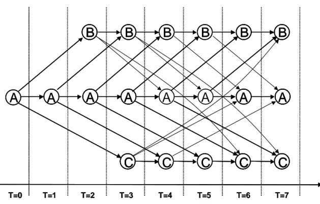
The Figure 2 depicted below shows the space-time graph over a time horizon of 7 periods, that means all the possible alternative movement strategies which lead to any DP starting from DP (A) at time T=0 . It is important to notice that the procedure for the determination of the optimal route provides for the carrier to wait in a certain DP simply by
A
B
2 3 4C
C
Distances between nodes: A-B: 2 periods of travel A-C: 3 periods of travel B-C: 4 periods of travel
indicating the same DP for the target movement for the next period of time.
Figure 2: space-time graph over a 7-period time horizon Each time a carrier passes through a DP its probability to catch an order increases; as a result, the expected profit ΠR of the route is determined by the expected profit Π0
j
(k, s) of the first movement towards the first deviation point, plus the expected profit of the second movement towards the second deviation point multiplied by the probability of not catching the order in the SA of the first DP, plus the expected profit of the third movement towards the third deviation point multiplied by the combined probability of not catching the order in the SAs of the first two DPs and so on until the time horizon is exhausted. The time horizon can be chosen for example equal to the fuel distance of the carrier. In accordance to what has been previously said, every time the
A
A
B
A
C
B
B
A
A
C
C
B
B
A
C
C
B
B
A
C
C
B
A
C
B
B
A
A
C
C
B
A
C
B
B
A
A
C
C
B
A
B
B
A
A
A
A
T=0 T=1 T=2 T=3 T=4 T=5 T=6 T=7A
A
B
B
A
A
C
C
B
B
A
A
C
C
B
B
A
C
C
B
B
A
C
C
B
B
A
A
C
C
B
B
A
A
C
C
B
B
A
A
C
C
B
B
A
A
C
C
B
B
A
A
B
B
A
A
A
A
T=0 T=1 T=2 T=3 T=4 T=5 T=6 T=7carrier reaches a DP, the time horizon is shifted ahead and the elaboration of the route must be repeated to update, besides other informations, the position of the other carriers of the fleet. The result is that the off-hire carrier is assigned a route intended as a sequence of movements and waits among the various DPs, which does not aim to any final target but only optimize the itinerary in the expectance of catching an order before the time horizon is exhausted; for this reason the strategy has been called “the Pilgrim Strategy”. The computation complexity of an algorithm which analyses all the possible routes (paths) on the space-time graph increases more than exponentially with the number of nodes of the network, that means with the length of the time horizon, with the number of DPs and with the number of carriers of the fleet. The search for the optimal route is a difficult problem and different methods have been suggested to solve the specific instance of the problem in the application case; some heuristics succeed in reducing the complexity of the problem to a polynomial order but for brevity purposes the description of these methods will be omitted. It is just noticeable that the expected profit of any route is upper bounded by the sum of the expected profits of the nodes included in the route itself. The algorithms for the search of the path which maximizes the sum of the weights of the nodes in a graph are numerous and all of them solve the problem in a polynomial number of steps. The exploitation of these algorithm, though it would not provide the optimal solution for our problem but only the upper bound, can be anyway helpful to the fleet manager as a Decision Support System.
6. APPLICATION OF THE MODEL
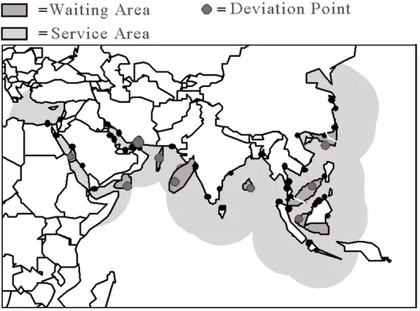
An application of the described model is under testing on a case of a oil-cargo company for on-demand transportation services. The aim is the route management of 12 ships in the South-East Asia / Middle-East zone in which there are more the 30 loading docks (PP). The scenario is showed in Figure 3, in which are put in evidence all the PPs, the various SAs, WAs and DPs.
Figure 3: snapshot of the selected area representation
The route is calculated on daily time unit and the time horizon is 20 days. The historical time series used for the determination of the order probabilities in each loading dock is related to the oil transportation services during the years ’93-’98 and an example of data representation is showed in Figure 4. Due to the low reliability of the naval
transportation, despite the speed of the modern tankers is approx. 12-13 knots, the average speed used in the model is vm = 10 knots; the main risks are due to unforeseeable events caused by malfunctioning or whether changes. The Time Windows has been chosen equal to 3 days: the competitiveness of the naval transportation segment indeed causes the order to be released by the customer up to 3-4 days in advance with respect from the departure date at the loading dock.
As an example of the determination of the order probability in a specific PP, here it follows the representation of the order probability used for the port of Singapore, obtained with the hypothesis of a Poisson distribution of the orders.
PSING(k,s) Mon Tue Thu Wed Fri Sat Sun
K=1 0.2212 0.1393 0.1813 0.1975 0.2592 0.0488 0.0100 K=2 0.0265 0.0102 0.0175 0.0209 0.0369 0.0012 0.0000 K=3 0.0022 0.0005 0.0011 0.0015 0.0036 0.0000 0.0000
Figure 4: example of data representation of the order probability in the Singapore PP
Experimentally some difficulties has been encountered in the manually modification of some WA in accordance to some specific requests of the tank-oil company; for example some parts of the Indonesian or Malaysian coasts or some expanses of sea in war-zones are carefully avoided to preserve the safety of the crew and the integrity of the load. The application of the model is giving satisfying results as a Decision Support System thanks to the fact that greatly reduces the alternatives of movements thus simplifying the tasks of the fleet manager.
7. REFERENCES
- W. B. Powell, Y. Sheffy, K. Nickerson: “Maximizing Profits for N. American Van Lines Truckload”, 1988, Interfaces 18, pp. 21-41 - W. B. Powell: “An operational planning model for the dynamic
vehicle allocation problem with uncertain demands", 1987 transportation research, Vol 213, n°3 pp. 217-232
- W. B. Powell: “A Stochastic Formulation of the dynamic
Assignment Problem…”, 1996
- M. W. P. Savelsbergh: “The General Pick-up and Delivery Problem”, 1995
- W. B. Powell, A. Odoni, P. Jaillet: “Stochastic and Dynamic Networks and Routing”, 1994