Three dimensional strain analysis of vertebrae with artificial metastases through digital volume correlation

(1)

ALMA MATER STUDIORUM -UNIVERSITA' DI BOLOGNA

CAMPUS DI CESENA

DIPARTIMENTO DI

INGEGNERIA DELL’ENERGIA ELETTRICA E DELL’INFORMAZIONE

“GUGLIELMO MARCONI”

CORSO DI LAUREA IN INGEGNERIA BIOMEDICA

Three dimensional strain analysis of vertebrae

with artificial metastases through digital

volume correlation

Elaborato in

Comportamento Meccanico dei Materiali (LT)

Relatore Presentata da

Chiar.mo Prof. Luca Cristofolini

Giulia De Donno

Correlatore

Dott. Marco Palanca

Dott. Enrico Dall’Ara

(2)

1

ABSTRACT

Bone is a common site for metastases and spine represent the most frequent site. Lytic lesions are associated with the loss of bone tissue, which can compromise the mechanical competence of the vertebra, leading to spine instability. Rigid stabilization is a solution, but it is a complex surgery, that can be very critical for oncologic patients; on the other hand, an untreated metastasis can lead to mechanical failure of the bone, leading to pain, immobilization and in the worst case, paralysis.

In this study, a protocol to analyse the strain with simulated lytic metastasis under compressive loading has been developed and optimized using a porcine vertebra. The strain distribution has been measured experimentally using micro-computed tomography (micro-CT) and Digital Volume Correlation (DVC), which provided three-dimensional displacements and strains maps inside the specimen. The ideal parameters for the DVC have been found by analysing two repeated scans in constant strain condition and setting a target of 200 microstrain for the errors (one order of magnitude lower than typical strains in bone subjected to physiological loading conditions). An ideal nodal spacing of 50 voxels (approximately 2 mm) has been chosen and a voxel detection algorithm has been applied to all data to remove regions outside the bone. In order to understand how the presence of the defect could alter the strain distribution, the porcine vertebra has also been subjected to non-destructive compressive load before and after the preparation of a mechanically induced lytic metastasis in the vertebral body. An increase of the 40% of the compressive principal strain after the defect has been found in proximity of the lesion.

This protocol will be used in future studies to analyse the effect of size and position of artificially metastatic lesions in the vertebral body of human spines.

(3)

2

1. INTRODUCTION

1.1 MOTIVATION

Bone is a common site of metastases for many primary malignant tumours, in fact approximately two-thirds of patients with cancer will develop bone metastasis. The spine represents the most frequent site of skeletal metastasis. (Guillevin et al., 2007, Maccauro et al., 2011).

When cancer spreads to the bone, it will make the bones weaker and even cause them to break without an injury; in fact, metastatic lesions are associated with the loss of bone tissue (lytic lesions) or formation of new tissue with poor mechanical properties (blastic lesions) (Whyne et al., 2000; Kaneko et al., 2004). Patients can have both osteolytic and osteoblastic metastasis or mixed lesions containing both elements. Rigid stabilization both relieves pain and prevents mechanical failure in metastatic disease. At the same time, stabilization involves surgical intervention, which could be quite demanding for the oncological patients (Choi et al., 2010; Ibrahim et al., 2008 Palanca et al., 2018). Understanding which lesions need treatment to prevent catastrophic failure is still an unsolved challenge.

The Spinal Instability Neoplastic Score (SINS) categorizes tumour related spinal instability. The total SINS (0-18 points), divide three clinical categories:

- stable: 0-6 points,

- potentially unstable: 7-12 points, - unstable: 13-18 points

A score of 0 to 6 denotes stability, 7 to 12 denotes indeterminate (possibly impending) instability, and 13 to 18 denotes instability. A surgical consultation is recommended for patients with SINS scores greater than 7 (Fisher et al., 2014). In this classification system, tumour-related instability is assessed by adding together six individual component scores: spine location, pain, lesion bone quality, radiographic alignment, vertebral body collapse, and posterolateral involvement of the spinal elements (Fourney et al., 2011).

(6)

5 Each patient case included a clinical history regarding pain, which is an important component of SINS. In the real world, history taking in this area may be more complex because of multiple sources of pain in patients with metastatic disease.

The inter- and intraobserver ICC reliability of final SINS categorization achieved near-perfect agreement. All subcategories had moderate to near-near-perfect agreement, with the exception of bone quality, which only had fair interobserver reliability and moderate intraobserver reliability. It could be possible to improve reliability by providing raters with multislice CT for every patient case (Fourney et al., 2011).

Because of the difficulty of accessing in vivo the musculoskeletal loads in the spine, in vitro measurements of the load-strain relationship in the vertebral body can provide valuable indirect information about spine biomechanics (Cristofolini et al., 2013). At that end, different techniques, such as strain gauges (Cristofolini et al., 2013) or Digital Image Correlation (Palanca et al., 2018) have been used to assess the strain distribution in the vertebra.

Recent studies made used DIC to evaluate the effect of mechanically induced vertebral metastases in human spine (Palanca et al., 2018). The specimens were first tested intact, then after the preparation of a defect in the vertebral body. The procedure was iterated for increasing size of the defect under compressive loads up to failure. The distribution of the strain was measured for lytic defect of increasing size and a threshold volume of defect that critically increase the strains was found. In that way, the region where the fracture would occur could be predicted based on the distribution of strain for non-destructive loads.

However, strain gauges and DIC can measure strain only on the external surface of the vertebra. On the other hand, Digital Volume Correlation (DVC) is a technique introduced by Bay and colleagues in the 1999 to measure displacement and strain inside the bone (Bay et al., 1999). DVC is a full field, contactless technique that provides both displacement and strain maps inside bone specimens via the comparison of 3D images of the undeformed and deformed object (Grassi and Isaksson, 2015). In this perspective, digital volume correlation (DVC) is ideal to investigate the local internal damage in treated vertebrae.

(7)

6 Many applications of the DVC to measure displacement and strain inside bone structures are reported in the literature (Bay et al., 1999; Liu and Morgan, 2007; Hussein et al., 2012; Gillard et al., 2014; Danesi et al., 2016 Palanca et al., 2016; Zhu et al., 2016; Tozzi et al., 2017). Two recent studies reported that high resolution images, based on synchrotron radiation (SR micro-CT), can improve the accuracy and precision of the DVC displacement and strain measurements (Christen et al., 2012; Palanca et al., 2017).

DVC was used to investigate the internal strain distribution of the vertebra in the elastic regime and up to failure (Tozzi et al., 2016). Two different DVC approaches were compared by using DVC to estimate local strain in natural and augmented vertebra, and to estimate the measurement uncertainties of bone and cement-bone interface in augmented vertebrae (Palanca et al., 2016; Tozzi et al., 2017); however, DVC was never used to evaluate the effect of bone lesions in the vertebrae, which is the aim of this study.

(8)

7

1.2 SPINE ANATOMY

The vertebral column forms the central axis of the body's skeleton. Superiorly, it articulates with the skull, and inferiorly, it articulates with the two hip bones, part of the lower limbs. Along with the sternum and the twelve pairs of ribs, it forms the skeleton of the trunk (Mahadevan, 2018).

The normal anatomy of the spine has been usually described by dividing the spine into 5 major sections the:

- Cervical, with 7 vertebrae (C1 – C7) - Thoracic, with 12 vertebrae (T1 – T12) - Lumbar, with 5 vertebrae (L1 – L5)

- Sacral, with 5 vertebrae fused together (S1 – S5) - Coccyx

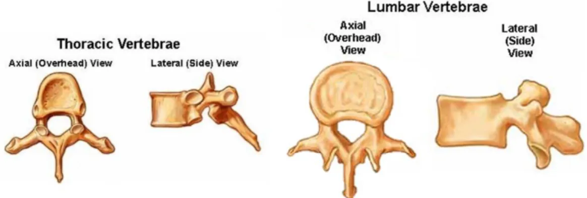
The neck (cervical) and low back (lumbar) region have a gentle convex curve (figure 1.2.a).

The vertebrae are 33 individual bones that interlock with each other to form the spinal column and only the top 24 bones are moveable, because the vertebrae of the sacrum and coccyx are fused.

(9)

8 The vertebrae in each region have unique features that help them perform their main functions:

- Cervical. The main function is to support the weight of the head. They grant a great range of motion because of the special shape of the first two vertebrae (figure 1.2.b). The C1 vertebra, also called atlas, is shaped like a ring and connects directly to the skull. This joint allows for the nodding motion of the head. The C2 vertebra has an upward-facing long bony process called the dens. The dens form a joint with the C1 vertebra and facilitates its turning motions. This joint allows for the side-to-side motion of the head.

- Thoracic. The main function of the thoracic spine is to hold the rib cage and protect the heart and lungs. The range of motion in the thoracic spine is limited (figure 1.2.c).

- Lumbar. The main function of the lumbar spine is to bear the weight of the body and for this reason, these vertebrae are much larger in size (figure 1.2.c).

- Sacrum. The main function of the sacrum is to connect the spine to the hipbones (iliac). There are five sacral vertebrae, which are fused together.

Figure 1.2.b Cervical vertebra C1 and

C2. Due to their particular shape, they allow great mobility at the neck.

(10)

9 An intervertebral disc connects one vertebral bone to the next. The discs are the shock-absorbing cushions between each vertebra of the spine. The disc is made up of two basic structures: the annulus fibrosus and the nucleus pulposus. The disc structures have different composition and function: the annulus is a tire-like structure that encases a gel-like center, the nucleus pulposus.

The annulus fibrosus enhances the spine’s rotational stability and helps to resist compressive stress. The nucleus pulposus is the soft, jelly-like center. It serves as the main shock absorber and is held in place by the outer annulus. The nucleus acts like a ball bearing during the movement, allowing the vertebral bodies to roll over the incompressible gel. Discs in the spine increase in size from the neck to the low back, as there are increasing needs for shock absorption due to weight, force reaction and gravity (figure 1.2.d).

Figure 1.2.c Representation of Thoracic and Lumbar vertebrae

(11)

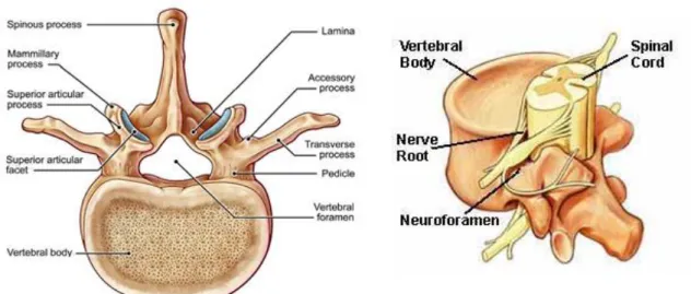
10 With the exception of the first two cervical vertebrae (atlas and axis respectively), all the moveable vertebrae, whether from the cervical, thoracic or lumbar regions, share a more-or-less common morphological design: vertebral body, vertebral arch (pedicles, lamina), and vertebral processes (spinous, transverse, and articular) (figure 1.2.f).

- Vertebral body - the large cylindrical part located anteriorly that gives strength to the spine. They are involved in load bearing. Their size increases from cranial to lumbar levels. Adjacent vertebral bodies are separated by intervertebral discs.

- Vertebral arch - the structure located posterior to the body. It consists of two pedicles and two laminae. The pedicles contain vertebral notches (superior, inferior) which form intervertebral foramina. These facilitate the passage of spinal nerves from the spinal cord (figure 1.2.f). The pedicles, laminae, and body of each vertebra form a cavity (vertebral foramen). The vertebral canal is the space throughout the spinal column that is enclosed by the vertebral foramina.

- Vertebral processes - there are seven in total all projecting from the vertebral arch: one spinous process (posteroinferior), two transverse processes (posterolateral), and four articular processes. The latter contain articular facets. The facet joints of the spine allow back motion. Each vertebra has four facet joints, one pair that connects to the vertebra above (superior facets) and one pair that connects to the vertebra below (inferior facets).

Figure 1.2.e The superior and

inferior facets connect each vertebra together. There are four facet joints associated with each vertebra.

(12)

11 The ligaments (figure 1.2.e) are strong fibrous bands that hold the vertebrae together, stabilize the spine, and protect the discs.

- The supraspinous ligament run between the tips of adjacent spinous processes.

- The interspinous ligament are sheets of fibrous tissue that run vertically in the midline between the facing borders of adjacent spinous processes and blend with the inner surface of the supraspinous ligament.

- The ligamenta flava span the gap between the facing borders of adjacent laminae (Mahadevan, 2018).

Figure 1.2.g Representation of the

ligaments in the spine

(13)

12 Due to limited availability of human cadaver spines, researchers are constantly seeking for representative animal models that reflect the biomechanical and anatomical characteristics of the human spine. Taking scaling differences into account, it is believed that the porcine spine can be a representative anatomical model for the human spine in specific research questions (Busscher et al., 2010). Many studies have been conducted with porcine vertebrae; for instance, they were used in order to understand strain distribution under different loading configuration (Cristofolini et al., 2013), to estimate local strains in natural and augmented vertebrae (Palanca et al., 2016) or to evaluate how the size of a simulated metastases affect the strain distribution on the anterior surface of the vertebra (Palanca et al., 2018).

Relating the dimensions to the size of the vertebral body, similarities were found in human and porcine vertebrae in the shape of the spinal canal, the transverse processes length, size of the pedicles and shape of the endplates.

In the human spine, all vertebral body heights generally increased from the cervical to the L3 vertebrae. In the porcine spine comparable heights were found, except for the posterior vertebral body height in the low thoracic and lumbar regions.

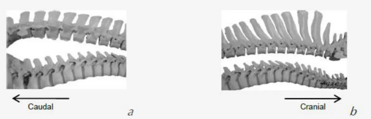
Human thoracic vertebrae had more pronounced transverse processes (figure 1.2.h).

The thoracic vertebrae of the porcine specimens studied had three distinct regions of differing geometry (figure 1.2.i): upper thoracic (T1–T2), middle thoracic (T3–T10)

Figure 1.2.h Porcine and human spines (a) The porcine (top) and human (bottom) lumbar spine show

comparable dimensions of pedicles and vertebral bodies and comparable behaviour. (b) Porcine (top) and human (bottom) thoracic spines show less similarity

(14)

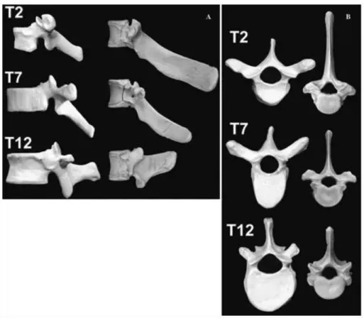
13 and lower thoracic (T11–T15 or −16). Although most porcine vertebral structures were smaller, porcine pedicle height was significantly greater than that of humans because the porcine pedicle houses a unique transverse foramen. (Bozkus et al., 2005). The vertebral body is smaller in size but has a similar shape.

The vertebral body enlarges through growth plates. These are cartilaginous rings on the top and the bottom of the vertebral bod. The cartilaginous rings expand and form bone. They are present in both human and porcine vertebra.

Figure 1.2.i Representative dried human (left) and porcine (right) vertebrae from the

upper thoracic region (T2), the middle thoracic region (T7), and the lower thoracic region (T12). A lateral views. B axial views. (Bozkus et al., 2005)

(15)

14

1.3 MICROCT

In recent years, the use of micro–computed tomography (microCT) imaging to assess trabecular and cortical bone morphology in animal and human specimens has grown widely. Although histologic analyses provide unique information indices of bone remodeling, they have limitations with respect to assessment of bone microarchitecture (Bouxsein et al., 2010).

MicroCT scanners capture a series of 2D planar X-ray images and reconstruct the data into 2D cross-sectional slices and these slices can be further processed into 3D models.

X-rays are emitted from an X-ray source and acquired by a detector. A specimen, mounted on a moving stage, is positioned between an X-ray source and a detector and the X-rays projections are acquired (figure 1.3.a).

There are two types of microCT systems:

- In ex vivo microCT systems usually the X-ray source and detector are fixed and the specimen rotates during the scans.

- In in vivo microCT systems, the X-ray source and the detector rotate around the animal or specimen.

Figure 1.3.a Key components and operating principle for standard desktop microCT scanner (Bouxsein et al. 2010). The X-ray generator emit the X-rays, they pass through the specimen and a planar detector record the unabsorbed X-rays. The projection will be later reconstructed via software.

(16)

15 After each projection is taken, the source and the detector (or the specimen) rotate by a fraction of a degree (typically 0.5 degrees or less) and the procedure is iterated until they have rotated of 180 or 360 degrees producing a series of projection images. Taking finer the step size, the resolution of the collected image will be higher.

The computer controls the X-ray source and specimen stage, obtaining X-ray projections at hundreds of angular positions. The X-ray absorption could be partial or differential. The partial adsorption means that some photons, emitted by the X-ray source, are adsorbed in the material while others are transmitted to the detector or deflected. The differential adsorption is based on the fact that different materials within the object have different absorption characteristic to give contrast.

The general form of X-ray attenuation is

𝐼

₁

= 𝐼

₀

∙ 𝑒

−𝜇 𝑡 Where:

- I0 is the X ray intensity before reaching the object

- e is the exponential coefficient - μ is the X ray attenuation coefficient - t is the thickness of the absorbing material

- I1 is the X ray intensity after passing through the object

The radiopacity of various objects and tissues results in radiographs showing different radiopacities, and hence they can be differentiated. Radiopaque tissues (such as a bone) will absorb more X-rays and result in a whiter image, whereas less radiopaque materials (like soft tissues or fluids) will results in a blacker image. For example, lead is used as a shielding material to stop X-rays, thanks to his high atomic number. In addition, thickness will lead to a poor transmission, because the X-rays will not have enough energy to pass though the sample and reach the detector. If the sample is not thick enough or it is not radiopaque, it will be difficult to image due to the low attenuation rate and the saturation of the detector.

(17)

16 MicroCT systems usually operate in a range of 20 to 100 kVp and the attenuation of the X‐ray photons as they pass through material can be caused by either absorption or scattering depending on their energy. The interaction of lower‐energy X‐rays (<50 keV) is dominated by the photoelectric effect and depends on the atomic number of the materials. This phenomenon is attributed to the transfer of energy from photons to electrons.

However, because the total attenuation of the X‐rays increases, only small objects can be measured at low energies, because otherwise noise becomes too large to allow quantitative analysis. The interaction of higher‐energy X‐rays (>90 keV) is dominated by Compton scattering, that occurs when the incident X-ray photon is deflected from its original path by an interaction with an electron. The electron is ejected from its orbital position and the X-ray photon loses energy because of the interaction but continues to travel through the material along an altered path.

In the medium range of X‐ray energy (50 to 90 keV), both the photoelectric effect and Compton scattering contribute to attenuation. (Bouxsein et al., 2010).

After acquiring the X-ray projection images, the computerised reconstruction of the 3D stack of images from the projection images is performed. The image reconstruction usually includes a beam hardening compensation. In fact, as a polychromatic X-ray beam passes through matter, low energy photons are preferentially absorbed, and the (logarithmic) attenuation is no longer a linear function of absorber thickness. This leads to various artefacts in reconstructive tomography that can be remedied by applying a linearization correction to the detector outputs. (Brooks and Di Chiro, 1976).

A voxel is defined as the discrete unit of the scan volume that is the result of the tomographic reconstruction; in fact, each three-dimensional voxel represents a specific X-ray absorption. The voxel size for microCT images is usually isotropic, which means that all the sides are the same dimension. The resolution of the image is defined as the smallest feature that can be resolved in the image. Hence, the resolution and voxel size are not equivalent but usually related.

(18)

17 Voxel size is a setting that can be chosen prior to the scan and has to be appropriately small compared to the dimensions of the structure being measured. Ideally, the smallest voxel size (highest scan resolution) available would be used for all microCT scans. However, high-resolution scans are not always desirable since they require longer acquisition times and generate large data sets (Christiansen, 2016), therefore a compromise between the minimum resolution acceptable and the scan time should be found.

1.4 STUDY AIM

Bone is a common site for metastases and the spine is the most frequent site. Rigid stabilization is a solution, but it is a complex surgery, that can be very critical for oncologic patient; on the other hand, an untreated metastasis can lead to mechanical failure of the bone, leading to pain, immobilization and in the worst case, paralysis. Understanding how metastases can influence the stability of the spine is crucial. Using DVC, we can gather information about the internal structure of the bone in a non-disruptive way and, through the strain distribution, understand which areas are weakened from the metastasis.

The aim to this study is to develop a procedure to evaluate how the strain distribution in the vertebral body is affected by the presence of simulated lytic metastasis using DVC with optimized parameters of scan.

(19)

18

2. MATERIALS AND METHODS

The study was divided into three parts. In the first part the optimisation of the DVC parameters was obtained by analysing repeated scans of a porcine vertebral body in constant strain conditions. In the second part, compressive loads were applied to the specimen in a time-lapsed manner. This allowed us to understand how the bone deformed under load up to 6500N. Finally, in the third part, a mechanically induced bone defect was prepared in the specimen and a compressive load to 6500N was applied again, to see how the presence of the defect would modify the distribution of principal strains in the vertebra.

2.1 SAMPLE DESCRIPTION AND PREPARATION

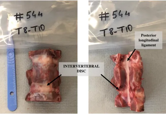
Specimen SP544 was obtained from a 9-month-old female pig (weight around 100 kg). A thoracic five-vertebral segment (T8-T12) was used (figure 2.1.a). The specimen did not have any sign of previous fracture, or other obvious defects, but growth plates were visible in the body of the vertebrae (figure 2.1.b). After defrosting the specimen for almost 5 hours at room temperature, most of the soft tissues around the vertebral body of the vertebra of each segment were removed using scalpel and pliers, while the posterior and the intervertebral disc were left intact. The five-vertebral segment was sawed in the middle to obtain two vertebral segments of equal dimension. The two vertebral segments were T8-T10 and T10-T12, where T8, T10 and T12 were cut mid-height. In this study, only the T8-T10 segment was analysed.

In order to create an in vitro procedure usable for human vertebrae it was decided to study only the vertebral body of the specimen. Tests were performed on the vertebral body due to the differences between the human vertebrae and pig vertebrae (arch and spinous process are larger in the porcine vertebrae), and because the whole human vertebra would not fit in the available testing jig and microCT field of view. Furthermore, the presence of the arch and facets would worsen the quality of the microCT images due to image artefacts.

The posterior elements of the three-vertebral segment were removed by performing two cuts in the vertebral arch by means of a handsaw (figure 2.1.b, figure 2.1.c).

(20)

19 During the whole procedure, the specimen was moisturized with water. When the procedure was complete, the specimen was put back in the freezer at approximately -25 °C.

Figure 2.1.a Specimen SP544,

thoracic vertebrae T8-T12. Specimen before any treatment.

Growth plates

VERTEBRAL ARCH VERTEBRAL

BODY

Figure 2.1.b Superior view of the specimen. Growth plates

are very visible. The dashed line indicates where the cut will be made to separate the body to the vertebral arch, after the removal of most of the soft tissues.

Figure 2.1.c Thoracic vertebrae T8-T10. All soft tissue has been removed, as well as the

arc and spinous process. The disc and ligaments are intact. INTERVERTEBRAL

DISC

Posterior longitudinal

(21)

20

2.1.1 EMBEDDING THE EXTREMITIES OF THE SPECIMEN IN RESIN

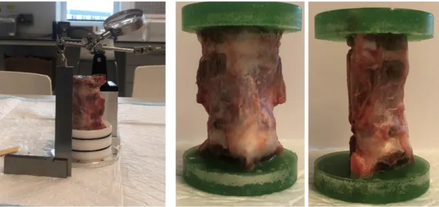
In order to hold the specimen in a controlled position, the vertebra was placed in a custom-made jig for the embedding in Polymethylmethacrylate (PMMA). The specimen’s transverse plane was aligned as parallel as possible to the middle vertebra endplates, the sagittal plane as perpendicular as possible to the plane of the endplate (figure 2.1.1.a).

Technovit 4071 (Heraeus Kulzer, Weinheim, Germany) is a two-component technical polymer, including a liquid and a powder, which is usually used in a ratio of 2:1 (powder/liquid). In this study, 20 g of powder and 13 g of activator were mixed carefully, trying not to create bubbles. The pot was greased with a release agent to ease the removal of the PMMA from the pot. The mix was poured into the pot, while trying not to move the specimen. After 25 minutes, the specimen with the first base of cement was removed from the pot. The specimen was glued at the superior pot of the jig. The inferior pot was filled with another mix of Technovit 4071 and activator. The superior pot was slowly made slide into the jig, until the superior face of the specimen was immersed in the mix.

Figure 2.1.1.a The specimen’s

transverse plane was aligned as parallel as possible to the endplates, the sagittal plane as perpendicular as possible to the plane of the endplate. PMMA was poured in the pot to embed the vertebra.

Figure 2.1.1.b Frontal and lateral vision of the specimen after

(22)

21 After 30 minutes, the specimen was removed from the jig (figure 2.1.1.b). The specimen was labelled and photographed. Once again, during the whole procedure, the specimen was moisturized with water and when the procedure was complete, the specimen was put back in the freezer at approximately -25 °C.

2.2 SETUP BEFORE ACQUISITION

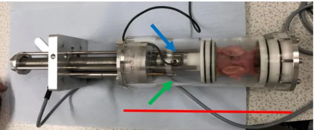
Before microCT scanning, the testing jig and related acquisition system were prepared for the test, as shown in figure 2.2.a. The force sensor was an HBM loadcell C9C (HBM, Germany), a compressive force transducer with a nominal full-range force of 10 kN. The displacement transducer was a LVDT (Linear Variable Displacement Transducer) with a measuring range of 20mm (HBM, Germany). The sensors were connected to a Spider8 amplifier (HBM, Germany), an electronic measuring system for PCs for electric measurement of mechanical variables. The signal was visualized and saved in a laptop through the “Catman Easy” software (HBM, Germany).

Catman data acquisition software (DAQ) allows for data visualization, analysis and storage during the measurement and reporting after.

LVDT 20mm (HBM) 10 kN loadcell (HBM) Sense 8 amplifier (HMB)

(23)

22 The output file consisted in a matrix of three columns (time (s), load measured by the loadcell (N), displacement measured by the LVDT (mm))

The jig was inserted into a metallic support for the application of the load and for positioning of the specimen during the scans. In the same support, the LVDT and Loadcell were inserted (figure 2.2.b) in order to measure the compressive load applied to the specimen and its axial displacement

By temporarily securing the metallic support to a plane surface, it was possible to apply compressive loads (by the use of a torque wrench) and waiting for the successive relaxation (figure 2.2.c).

Afterwards, all hardware was connected, the LVDT and the Loadcell were both zeroed. The acquisition rate was set to 50Hz for the loading steps and 1Hz during the scans.

Figure 2.2.c The metallic support is secured to a

plane surface. Using a torque wrench is possible to apply compressive loads by turning the screw of the support.

. Figure 2.2.bJig (in red) on a metallic support to permit loads and positioning in the scan machine. The Loadcell (blue arrow) and the LVDT (green arrow), are used to quantify the compressive load (and displacement) on the specimen

(24)

23

2.3 ACQUISITION OF MICROCT IMAGES AND TIME LAPSED TEST A microCT scanner (VivaCT80, Scanco Medical, Switzerland) was used to acquire high resolution images of the specimen before and after loading. The following scanning parameters were used (“METVERT” project): voltage 70 kVp, current 114 μA, power 8 W, exposure time of 300 ms and voxel size 39 μm.

A scout view was performed to define the reference line for the acquisition of the interested regions of interest. Each scan took approximately 1h.

The images were reconstructed using the software provided by the manufacturer and applying a beam hardening correction based on a phantom with 1200 mg HA/cc density.

2.3.1 APPLICATION OF THE LOADS

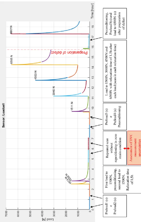
As is shown in figure 2.3.1, compressive loads were applied to the specimen in a time-lapsed manner.

A preload of approximately 20N was applied and two consecutive images (“Preload1” and “Preload2”) were acquired. Afterwards, a load until 1500N was made and right after ten preconditioning cycles (30-300N) were applied, followed by a second load until 1500N and 1.5h of relaxation time. Then, two repeated scans (“Load2a”,

“Load2b”) withour repositioning were performed at approximately 130N (small load) to evaluate the uncertainties of the DVC approach (figure A1).

Finally, two repeated scans (“Preload3” and “Preload4”) were made to a preload of approximately 20N and right after, ten preconditioning cycles (30-300N) were made. Then different loading steps were applied in a time-lapsed manner until 1500N, 3000N, 4500N and 6500N, respectively (scans called: “Load1500N”, “Load3000N”, “Load4500N”, “Load6500N”). Each load step started was followed by relaxation time of 1.5h, where a scan was made for each step (figure A2).

(25)

24

Figure 2.3.1 Description of the compressive loads applied to the specimen. In the first part of the study,

there was an assessment of DVC measurement uncertainties, in the second and third parts, compressive loads were applied before and after the preparation of the defect. The symbol (s) shows where the scans were made.

(26)

25 2.4 IMAGE PROCESSING

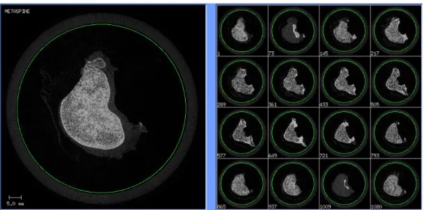
The collected projections (X-rays) are then reconstructed automatically by the software provided by the microCT manufacturer. Afterwards, the software “MobaXTerm” was used to visualize the slices of the reconstructed 3D image, to crop the images and to convert the data in 16-bit multislice DICOM files (figure 2.4). It was possible to download the images with the “Scanco medical MicroctFTP” software. The file size for each scan is approximately 6 GB.

In order to improve the handling of the datasets, the images were converted into 8-bit DICOM files by using the software “ImageJ” (National Institutes of Health and the Laboratory for Optical and Computational Instrumentation (LOCI, University of Wisconsin) and the “Tudor DICOM plugin”. Finally, the central vertebra was isolated by cropping the disks and superior and inferior endplates of the vertebrae embedded in the PMMA.

Figure 2.4 Example of the result of the scan after reconstruction in MobaXTerm. It is possible to see

a preview of the slices and it allows to crop the images (green circle), in order to partially eliminate the unnecessary parts of the scan.

(27)

26

2.4.1 CREATION OF THE IMAGE MASK

A Gaussian Blur 3D (X sigma =3, Y sigma=3, Z sigma=3; ImageJ) was applied to the 8 bit-image(figure 2.4.1.b) to reduce the high-frequency noise (Bouxsein et al., 2010). Image segmentation was performed followed by a single-level threshold in the valley between the first two peaks of the greyscale histogram. The threshold was adjusted visually by comparing the segmented and greyscale images (Palanca et al., 2017). The result was a binary image that had a bit value of 0 in the background and 255 in the bone (figure 2.4.1.c). The binary processes “Dilate” and “Fill Holes” were used as many times as needed, to fill all the internal holes of the vertebra, resulting in a mask like the one in figure 2.4.1.d. The quality of the mask was then checked in all slices.

Figure 2.4.1.a Original image Figure 2.4.1.b Image after the Gaussian

Blur 3D is applied (3,3,3).

Figure 2.4.1.c Image with the adjusted

threshold. The bone must have a value of 255 and the background of 0.

Figure 2.4.1.d Finished mask after the

binary effects “Dilate” and “Fill Holes”

(28)

27

2.4.2 RIGID REGISTRATION

Rigid image registration is the process of transforming different sets of data into one coordinate system. One image is fixed (the reference image), whereas the other (the moved image) is spatially transformed to match it. A rigid-body transformation in three dimensions is defined by six parameters: three translations and three rotations. The source is then re-sampled at the new positions.

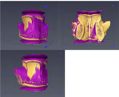
The fixed and moved images were loaded in Amira (Amira6.0.0, Thermo Fisher Scientific) as “LDA” (Large Data Set). Once loaded, a subvolume was extracted from the images (max width, max height, max depth) with a subsampling of 2 in each direction. By generating the isosurfaces for both images, it was possible to visualize and manually pre-align the images (figure 2.4.2). The registration was made and a matrix of values (3 rotations and 3 translation) was acquired. Now it was possible to impose this matrix to the moved whole image (not LDA format) and resample the two whole images together. The image form Amira was saved in a DICOM 8-bit multi-slice file and using ImageJ it was possible to convert it in a DICOM 8-bit file.

Figure 2.4.2 Images before the rigid registration. The fixed image (yellow) and the moved image

(purple) have slightly different position. The rigid body registration will rotate and translate the moved image until they are aligned. The resampling will rewrite the grid of the moved image in the fixed one.

(29)

28

2.5 BONEDVC ANALYSES

After the creation of the mask, it was possible to proceed with the registration of the images for the evaluation of the displacements and strains in the vertebral body. The BoneDVC service was used for this purpose (https://bonedvc.insigneo.org/dvc/ ). The BoneDVC service, previously known as ShIRT-FE, consists of a home-written elastic registration software based on the Sheffield Image Registration Toolkit (ShIRT, Barber and Hose, 2005; Barber et al., 2007) and a Finite Element (FE) software package (ANSYS mechanical APDL v. 14.0, Ansys, Inc., USA).

The procedure focuses on finding the displacement map that minimises the differences between the two 3D images (called the fixed and moved images). The problem is to find the displacement functions u(x, y, z), v(x, y, z) and w(x, y, z) that map each point in the fixed image f(x, y, z) (with coordinates x, y, z) into those in the moved image m(x’, y’, z’) (with coordinated x’= x+u, y’= y+v, z’= z+w) . As described in Barber et al., 2007, additional intensity displacement function c(x, y, z) is included in order to account for changes in the grey levels. For small displacement values, we need to solve: 𝒇(𝑥, 𝑦, 𝑧) − 𝒎(𝑥, 𝑦, 𝑧) ≈1 2(𝑢 ( 𝜕𝒇 𝜕𝑥 + 𝜕𝒎 𝜕𝑥) + 𝑣 ( 𝜕𝒇 𝜕𝑦+ 𝜕𝒎 𝜕𝑦) + 𝑤 ( 𝜕𝒇 𝜕𝑧+ 𝜕𝒎 𝜕𝑧) − 𝑐(𝒇 + 𝒎)) (1)

However, as this problem would be underdetermined if solved for each voxel, ShIRT solves the equations only in the nodes of a cubic grid superimposed to the images and with elements as large as the imposed subvolume. The displacements are interpolated with a trilinear function between the nodes.

𝑢(𝑥, 𝑦, 𝑧) = ∑ 𝑎𝑥𝑖 𝜑𝑖 (𝑥, 𝑦, 𝑧) 𝑖 𝑣(𝑥, 𝑦, 𝑧) = ∑ 𝑎𝑦𝑖 𝜑𝑖 (𝑥, 𝑦, 𝑧) 𝑖 𝑤(𝑥, 𝑦, 𝑧) = ∑ 𝑎𝑧𝑖 𝜑𝑖 (𝑥, 𝑦, 𝑧) 𝑖

(30)

29 In the equations the term φi (x, y, z) is the ith basis function centred at the node with coordinate 𝑥𝑖, 𝑦𝑖, 𝑧𝑖. The problem is then solved when the coefficients 𝑎𝑗𝑖 of the displacement function are found.

The Equation (1) can be now written in matrix notation (capital letters represent tensors, low case letters represent vectors) as:

𝒇 − 𝒎 = 𝑻𝒂 (2)

where the matrix T is derived from integrals of the image gradients multiplied by the basis functions.

ShIRT adds an additional smoothness constraint on the mapping by including in the solution a term based on the Laplacian operator L, and the coefficient λ that weights the relative importance of smoothing. The result of adding this constraint is to convert the equation (2) to the form:

(𝒇 − 𝒎) = (𝑻𝑻_{𝑻 + 𝜆𝑳}𝑻_𝑳)𝒂

where T is a K × N matrix (K is the number of voxels in the image, and N is the number of nodes in the grid). T is derived from integrals of the image gradients multiplied by the basis functions of the displacements. For large displacements, the method can iterate to a correct solution as shown in Barber et al., 2007. The grid is then converted into an eight-node hexahedrons mesh.

After that, the six components of strain at each node of the grid are computed by differentiating the displacement field with ANSYS. The strain vector for a three-dimensional domain is given by

{𝜺} = [ 𝜀_𝑥 𝜀_𝑦 𝜀_𝑧 𝛾_𝑥𝑦 𝛾_𝑦𝑧 𝛾_𝑥𝑧 ]𝑇

where εx , εy and 𝜀𝑧 are the normal strain component and 𝛾𝑥𝑦, 𝛾𝑦𝑧 and 𝛾xy are the shear strain components, expressed as partial derivatives of the displacements u, v and w. 𝜀_𝑥= 𝜕𝑢 𝜕𝑥 εy = ∂v ∂y εz = ∂w ∂z γ_xy = ∂u ∂y+ ∂v ∂x γyz = ∂v ∂z+ ∂w ∂y γxz= ∂w ∂x + ∂u ∂z

(31)

30 The BoneDVC service use as inputs:

- a fixed image: the image that will be the reference, the undeformed specimen - one or more moved and deformed image(s): the image(s) of the deformed

specimen

- a mask image: an image with 1 inside the contour of the vertebra and 0 outside, used to avoid registering portion of the image in not-interesting regions. - voxel size: dimension of the voxel in the images to be registered in microns - nodal spacing (NS): that defines a 3D grid of nodes at a distance of NS voxels

from each other that are used to solve the registration equations. More than one value can be provided.

- number of iterations: number of iterations after which to stop the registration algorithm in case it has not converged (different values for different NSs can be provided). Default value is 100.

The three images must be uploaded as 8-bit DICOM files, with the same dimension (number of voxels in each Cartesian direction). The images should have been already rigidly co-registered to improve the computational time.

The BoneDVC service gives as output a series of “.txt” files as descripted in the list below:

- list of elements (elements.txt) - list of node coordinates (nodes.txt)

- list of nodes coordinates and corresponding displacements along x, y and z directions (output_map.txt)

- list of displacement applied to each node (disp.txt), from output_map.txt - list of strains in the three directions computed at the nodes (results_xyz.txt) and

elements (results_elements_xyz.txt) in global coordinates

- list of principal strains computed at the nodes (results.txt) and at the elements (results_elements.txt)

- configuration file used for the analyses (configuration_file.txt) - log file(s) written during the analyses (cronLog-*.txt)

(32)

31 The BoneDVC service uses the algorithm proposed by Dall’Ara et al., 2014, which has been tested for several bone structures and was found to be more accurate than other published or commercially available alternative (Dall’Ara et al., 2017; Palanca et al., 2015)

In the first part of this study, the two images from the repeated scan (“Load2a” and “Load2b”) without repositioning in constant strain condition were registered in order to quantify the measurement uncertainties (figure 2.5.a, DVC_Load2a)

In the second part, after a series of increasing loads were applied, four images (for the four steps, “Load1500N”, “Load300N”, “Load4500N”, “load6500N”) were registered, in order to understand how the strain distribution changed after increasing loads (figure 2.5.a, DVC_Load1500N, DVC_Load3000N, DVC_Load4500N, DVC_Load6500N).

Figure 2.5.a. In blue, the DVC analyses utilized to study uncertainties of measurement (DVC_Load2a).

In green, the DVC results for studying strain distribution in the vertebra, under time lapsed loads. In the third part, in green, the data was used to compare principal strain distribution before and after the preparation of a defect (DVC_Load6500N vs DVC_Load6500NDEF)

(33)

32 After the preparation of the defect (See section 2.6), another registration was made (figure 2.5.a, DVC_Load6500NDEF). Comparing the values of the principal strain for this registration with the one without defect (DVC_Load6500N), it was possible to understand how the presence of the defect would change the principal strain distribution.

A voxel detection algorithm was applied to each result in order to analyse only strain values within the bone, as shown in (figure 2.5.b). This algorithm recognises which node is within the image mask and removes all the elements with at least one node outside the mask. Using the new set of data made only of nodes coming from the area of interest, we can now exclude all the values that were affected by the image noise outside the vertebra.

The two repeated scans without repositioning at constant strain condition (Load2a and Load2b) were analysed with the BoneDVC service, with a nodal spacing of 10, 30, 50, 70 and 90 voxels (figure 2.5.c), giving as a result the DVC analysis named DVC_Load2a. In this test, being in a constant-strain configuration (assumed in this experiment close to zero strain considering the low load in the first loading step before

Figure 2.5.b Effect of voxel detection. In this example, a microCT image is shown under the

corresponding grid of nodes from DVC, with a nodal spacing of 50 voxels. In the figure on the left (before voxel detection), the entire grid of nodes is shown in red. The picture on the right, instead, shows the effect of voxel detection. The majority of the nodes outside the area of interest (bone) is in fact excluded from the grid (shown in blue).

(34)

33 the images for this analyses were acquired), any strain different from zero was accounted as measurement error.

Measurement precision must also be considered in the context of total amount of signal within typical samples. For trabecular bone, the very earliest evidence of yielding begins at nominal strain of approximately 0.006 (6000 microstrain), and macroscopic local failure does not begin until a strain of 0.01 (10,000 microstrain) (Keaveny et al., 1994). A range for the typical physiological deformations is 1,000–2,000 microstrain (Yang et al., 2011), so the goal of this first step of the study was to keep the uncertainties at least one order of magnitude lower, at approximately 200 microstrain, in order to use the DVC also for the measurement of strain related to physiological loads. In order to do that, the SDER (Standard Deviation of the Error) was calculated for each nodal spacing for the repeated scan without repositioning in constant strain condition.

Figure 2.5.c1 Figure 2.5.c2 Figure 2.5.c3

Figure 2.5.c Schematic representation of the homogeneous cubic grid at different nodal spacing (NS)

imposed on a microCT image with a voxel size of 0.39 μm. Figure 2.5.c1 Nodal Spacing 10. Voxel dimension: 0.39mm Figure 2.5.c2 Nodal Spacing 50. Voxel dimension: 1.95mm Figure 2.5.c3 Nodal Spacing 90. Voxel dimension 6.3mm

(35)

34 From the output map of the DVC (a .txt file that indicates the position of each node in the image, (see section 2.5), the height of the vertebra was measured and divided into five “slices” (figure 2.5.d). Accuracy and precision were calculated for each component of strain in each node and averaged for each slice, in order to study the measurement uncertainties in different parts of the vertebra.

Each slice consisted of 4-5 planes and a total of approximately 1300 nodes (figure 2.5.d)

Figure 2.5.d On the left, a lateral image of the vertebra divided in slices. On the right,

the results directly from the output map after voxel detection. With a nodal spacing of 50 voxels, the vertebra is analysed in 6743 nodes, with around 1300 nodes for slice.

(36)

35

2.6 PREPARATION OF THE DEFECT AND IMAGING

With a handsaw, the embedding material of the specimen was carefully cut in order to stably fix it in the clamp of the vice (figure 2.6.a). A pillar drill (Sealeym, model no. GDM50BX) was used to produce a bone defect (lytic lesion) using a core drill with diamond coating (diameter equal to 8mm). The core drill was placed roughly in the middle of the anterior portion of the vertebral body, coring around 4 mm of bone along the left-right direction (figure 2.6.b). During the whole procedure, the specimen was irrigated with cold water in order to maintain low the temperature of the bone and avoid tissue damage.

In the third part of this study, after the preparation of defect, after a scan at around 100N, a compressive load up to 6500N was applied (figure A3).

A registration (“DVC_Load6500NDEF”) of the image with BoneDVC service was made, using the scan of the preload (“preload5”) as fixed image and the scan at 6500N image (“Load6500NDEF”) as moved image (figure 2.5.a).

Figure 2.6.a Cuts made

in the embedding material

(37)

36 The deformation of the specimens under a load of 6500N were compared before and after the mechanical application of a defect (DVC_Load6500N and DVC_Load6500NDEF). The results are presented for each component of the strain in each of the five slices considered.Considering that the specimen was taken out of the machine for the preparation of the defect, the analysis for each strain component in the global coordinates system would be affected by the relative position of the specimen in the testing jig. Therefore, in this part of the study only the principal strain of the specimen will be evaluated, with particular emphasis on the third principal compressive strain (E3).

As in the previous analyses, the height of the vertebra was calculated from the output map and for each registration (DVC_Load6500N and DVC_Load6500NDEF), the appropriate number of nodes was selected.

Standard deviation and mean values have been calculated for each component and shown in figure 3.5.a and figure A5.

(38)

37

2.7 METRICS

The accuracy and precision of the principal strain and strain in global coordinate were defined as mean and standard deviation of the computed strain values. The analyses were performed on the DVC_Load2a data to quantify:

- Optimal DVC parameters: accuracy and precision of the strain were calculated for each nodal spacing (10, 30, 50, 70, 90 voxels). Given the constant-strain condition (assumed in this experiment close to zero strain considering the low load in the first loading step before the images for these analyses were acquired), any strain value different from zero was accounted as an error. The following analyses were carried out:

- Accuracy and precision before and after the application of the voxel detection algorithm for each nodal spacing and component of strain (table 3.1.a, table 3.1.b). All further analyses will be made on data with the voxel detection algorithm (VD) applied.

- Comparison by component of each NS: to evaluate how different nodal spacing would affect precision and accuracy of the measurement. - Scalar comparison: following the indications available in literature

(Dall’Ara et al., 2014; Liu and Morgan, 2007), standard deviation of the error (SDER) was quantified as the SD of the average of the absolute values of the six strain components for each nodal spacing. The value of the optimal nodal spacing was found from this analysis by fitting the data with power laws.

After assessing the optimal scan condition (nodal spacing of 50 voxel and VD applied), DVC_Load2a was analysed for:

- Heterogeneity of the error. The specimen was divided in five horizontal slices (figure 2.5.d) and precision and accuracy were calculated for each slice, in order to study the measurement uncertainties in different parts of the vertebra. In the second part of the study, time-lapsed loads were applied. The DVC data DVC_Load1500N, DVC_Load3000N, DVC_Load4500N, DVC_Load6500N were

(39)

38 compared to show how strain distribution changes in each component at increasing loads.

The results of the scans at load until 6500N were compared before and after the preparation of defect (DVC_Load6500N and DVC_Load6500NDEF) for each component with she specimen divided in five even slices. Accuracy and precision were compared in each scenario.

(40)

39

3. RESULTS

3.1 EFFECT OF VOXEL DETECTION

The voxel detection algorithm (VD) excludes from the grid all the nodes that are outside the area of interest (figure 2.5.b). Intable 3.1.a and table 3.1.b, different values of accuracy and precision (mean and standard deviation), MAER (mean absolute error) and SDER (standard deviation of the error) for normal and shear strain component before and after voxel detection are reported.

As expected, the larger the subvolume, the lower the error (Palanca et al., 2015). This trend is shown in both datasets from pre- and post- VD and for both systematic and random error. After the VD a modest increase of the mean errors was noticeable, whereas the SD values were very similar. The exception was for NS 10, where both mean and SD values increased.

All further analyses were performed with data after the voxel detection algorithm in order to evaluate the uncertainties of the DVC algorithm within the region of interest.

Accuracy Without Voxel Detection

Nodal spacing [voxel] Ex [microstrain] Ey [microstrain] Ez [microstrain] Exy [microstrain] Eyz [microstrain] Exz [microstrain] MAER [microstrain] 10 79 178 -103 -48 -58 111 5473 30 89 160 -98 -43 -55 101 353 50 83 134 -94 -35 -56 108 195 70 68 118 -84 -34 -41 92 151 90 64 94 -77 -28 -40 90 118

With Voxel Detection

Nodal spacing [voxel] Ex [microstrain] Ey [microstrain] Ez [microstrain] Exy [microstrain] Eyz [microstrain] Exz [microstrain] MAER [microstrain] 10 163 167 -86 -104 -49 69 8027 30 119 137 -110 -52 -63 119 449 50 113 160 -102 -53 -53 113 227 70 103 158 -94 -48 -39 103 180 90 84 124 -89 -40 -33 84 139

Table 3.1.a Accuracy (mean value) and MAER (mean absolute error) were reported for different nodal

spacing. (10, 30, 50, 70, 90 voxels), for repeated scans in constant strain condition. As expected, both systematic and random error were lower for higher voxel dimension. After the application of the voxel detection algorithm, the mean values were slightly higher (especially for values at NS of 10 voxels).

(41)

40

Precision Without Voxel Detection

Nodal spacing [voxel] Ex [microstrain] Ey [microstrain] Ez [microstrain] Exy [microstrain] Eyz [microstrain] Exz [microstrain] SDER [microstrain] 10 6062 5663 5687 9384 8899 9309 3065 30 411 546 325 644 512 546 217 50 214 361 156 367 269 295 136 70 157 290 118 279 208 232 111 90 105 209 89 197 156 183 80

With Voxel Detection

Nodal spacing [voxel] Ex [microstrain] Ey [microstrain] Ez [microstrain] Exy [microstrain] Eyz [microstrain] Exz [microstrain] MAER [microstrain] 10 8420 7826 7468 13271 12275 12876 3299 30 539 569 414 766 628 539 216 50 268 408 190 398 305 268 148 70 192 352 141 310 237 192 122 90 127 256 107 221 177 127 89

Table 3.1.b Precision (standard deviation) and SDER (standard deviation of the error) were reported for

different nodal spacing. (10, 30, 50, 70, 90 voxels), for repeated scans in constant strain condition. As expected, both systematic and random error were lower for higher voxel dimension. The values of the standard deviation remained similar (except for values at NS 10 voxels that increased).

Figure 3.1.c Direction of the axis for the strain

(42)

41

3.2 EFFECT OF NODAL SPACING

The choice of the nodal spacing highly influence accuracy and precision, but also the computational time. In figure 2.5.b a qualitative representation of the superimposed grid with 10, 50 and 90 voxels is showed. Low nodal spacing lead to high resolution of the DVC measurements, but it also required longer computation time (table 3.2.a). As expected, the computational time rose dramatically with a higher number of sub-volumes, as the software has to elaborate a larger dataset (calculation of the displacements in each node of the grid and calculation of principal strains, normal and shear strain components in each node and centroid, see section 2.5).

An excessively large nodal spacing may result in an inadequate spatial resolution, whilst sub-volume size that is too small is typically susceptible to noise (Yaofeng and Pang, 2007). Therefore, a compromise must always be accepted between the precision of the DVC measurements and its spatial resolution.

NODAL SPACING (voxel) NODAL SPACING (mm)

MATRIX [X,Y,Z] NUMBER

OF NODES

COMPUT. TIME [h] Nodes for each plane

[X,Y] Number of planes [Z] 10 0.39 14’859 [127,117 ] 97 1441323 11.3 30 1.17 1763 [43,41] 33 58179 5.8 50 1.95 675 [27,25] 21 14175 5.8 70 2.73 361 [19,19] 15 5415 3.9 90 3.51 215 [15,15] 13 2925 3.9

Table 3.2.a Data from a repeated scan in constant strain condition without repositioning

(DVC_Load2a). In this table the relation between nodal spacing (in voxel and mm) and the dimension of the 3D matrix that contains thenodes before voxel detection is shown. A lower nodal spacing indicates a higher resolution and a larger amount of data. It is also shown the relation between the number of nodes and the computational time.

(43)

42

Figure 3.2.b Precision and accuracy after voxel detection for a repeated scan in constant strain

condition without repositioning. As expected, both systematic and random error were lower for higher voxel dimension. The accuracy for all components for nodal spacing has similar absolute value for each nodal spacing (33 – 167 microstrain). The precision was worse (higher error) especially for nodal spacing 10, where the error at least 2 orders of magnitude higher compared to those obtained for nodal spacing between 30 and 90 voxels.

(44)

43 Therefore, in order to compute the measurement errors, five sub-volume sizes (10, 30, 50, 70, 90 voxels) were investigated in two scans acquired under constant strain condition, (DVC_Load2a, as it shown infigure 2.5.a). The results of the analysis are shown in figure 3.2.b(data intable 3.1.a and table 3.1.b).

The accuracy for all components was similar for each NS (33 – 167 microstrain), whilst the precision was associated to higher errors for low nodal spacing. In particular, high errors were found for NS equal to 10, where the errors were at least two orders of magnitude higher compared to those for NS between 30 and 90 voxels.

The mean values for the shear component were lower, but their standard deviation was higher, especially in the nodal spacing 10, where the standard deviation values for the shear strain are almost doubled. The component with higher precision was Ez, the normal component in the Z direction.

Following the indications available in the literature (Dall’Ara et al., 2014; Liu and Morgan, 2007), the SDER (Standard Deviation of the Error) was calculated for each nodal spacing for the repeated scan without repositioning in constant strain condition (DVC_Load2a). As we can see in figure 3.2.c, the relationship between precision in measuring the strain and the NS were best approximate with a power law (R2=0.9406). Considering that the typical physiological deformations in bone is 1,000–2,000 microstrain (Yang et al., 2011), the goal of this first part of the study was to keep the DVC uncertainties at least one order of magnitude lower than typical strains in bone subjected to physiological loading conditions, at approximately 200 microstrain. Therefore, for NS between 10 and 30 voxels uncertainties were too high. Solving the equation for a value of SDER of 200 microstrain, we obtained an ideal nodal spacing dimension of 44 voxels. Therefore, the final choice for further analyses was a NS equal to 50 voxels.

𝑆𝐷𝐸𝑅 = 98633 𝑁𝑆−1.638 200 𝜇Ɛ = 98633 𝑁𝑆−1.638

(45)

44

Figure 3.2.c Relationship between precision in the strain and the nodal spacing

it can be approximated with power laws (R2_{=0.9406). In the figure we can easily}

visualize which nodal spacing has an error too large to be useful for our study (10, 30 voxels).

(46)

45

3.3 HETEROGENEITY OF ERROR WITHIN THE SPECIMEN

Using a nodal spacing of 50 voxel (1.95 mm) and applying the voxel detection algorithm to the nodes, the best compromise between resolution and error was found. The next step of the study was to evaluate if the distribution of the error was heterogeneous in the vertebra for the different slices considered.

Each slice had around 1300 nodes, and it consisted in 4-5 planes each (figure 2.5.d,

figure 3.1.c).

Figure 3.3.a Analysis on DVC_Load2a divided in five slices (slice 5 most cranial, slice 1 most caudal).

Each slice has approximately 1300 nodes. While the values of accuracy vary significantly, the precision does not seem to be dependent from the position in the vertebra.

(47)

46 The strain component with the lowest systematic and random errors was Ez, with three slices with values of accuracy under 40 microstrain and values of precision less than half compared to the other components (figure 3.3.a). For most components of strain, no clear trend was found between the values of the random or systematic errors and the position of the nodes in the vertebrae. However, for Ez the systematic and random errors were lower for the most caudal slice (slice 1) compared to the most cranial one (slice 5).

Figure 3.3.b Frequency plot for the components of error for each slice with NS of

50 voxels. Similar trends for each slice are visible. We can see that each component has a large deviation standard, especially Exz. Exy shows higher peak, whereas Ey has the lowest.

(48)

47 The components with the worst values of accuracy and precision were Ey and Exy but the frequency plot of Exy has higher peaks, while Ey has the lowest (figure 3.3.band in the figure A4). .Exz, Eyz and Ez showed particularly spread values and it appears that the most caudal slices had the highest peak compared to the cranial one.

It is interesting to notice that the accuracy for the shear strains had different sign for slice 1 and that the systematic errors for Ez were lower for slices 1-3 compared to slices 4-5. The component that showed less dependency from the position in the vertebra is Ey, with similar values of accuracy and precision in each slice.

(49)

48 3.4 ANALYSES OF STRAINS FOR INCREASING LOADS

During the second part of the study, compressive loads were applied in a time-lapsed manner (see section 2.3.1).

Figure 3.4.a In the second part of the study, compressive loads from 1500N up to 6500N were

applied (see section 2.3.1). As expected, the strain components increased with the loads in both mean value and standard deviation. The values of the zero-strain condition (DVC_Preload3) are used in comparison, to evaluate the uncertainties in the measurement.

(50)

49 The preload was analysed to show the uncertainties of the measurement. For each component the accuracy measured in zero strain condition (DVC_Preload3) had value up to -114 and 243 microstrain while the standard deviation varied from 324 to 461 microstrain, (table 3.4.b)

The analyses were performed for loads up to approximately 1500N, 3000N, 4500N and 6500N. As expected, the normal component of strain along the loading direction (Ez) increased with the load. Similar trends were observed for some of the other components (Ex, Exy, Eyz), whereas Ey did not seem to be dependent to the magnitude of the loads. The shear component Exz fluctuated in both magnitude and sign at each step.

The standard deviation rose at every load up to 9905 microstrain (Ez). All the shear strain components at a load until 6500N had high values of standard deviation, higher than those calculated from normal components Ex and Ey.

Time lapsed loading experiment Mean Ex [microstrain] Ey [microstrain] Ez [microstrain] Exy [microstrain] Eyz [microstrain] Exz [microstrain] Preload3 -67 -114 243 48 -35 -30 Load1500N 753 1004 -3240 124 -593 94 Load3000N 756 1016 -4044 200 -746 -45 Load4500N 1314 802 -5224 831 -265 -243 Load6500N 3624 1217 -8755 2526 -2998 384 Standard deviation Ex [microstrain] Ey [microstrain] Ez [microstrain] Exy [microstrain] Eyz [microstrain] Exz [microstrain] Preload3 380 355 324 437 415 461 Load1500N 1880 1791 3808 2147 2550 2128 Load3000N 1672 1581 5124 2369 3121 2844 Load4500N 2082 1590 6861 2904 4619 4208 Load6500N 5805 3627 9905 6457 8550 7056

(51)

50

3.5 ANALYSES WITH MECHANICALLY INDUCED DEFECT

The deformation of the vertebra loaded at approximately 6500N before and after the preparation of defect (DVC_Load6500N and DVC_Load6500NDEF) was compared. Analyses were performed for each principal strain in the different considered regions (figure 2.5.d).

As in the previous analysis, the height of the vertebra was calculated from the output map and for each registration (DVC_Load6500N and DVC_Load6500NDEF), the appropriate number of nodes was selected. Each slice had approximately the same quantity of nodes.

Standard deviation and mean values of the principal strains have been calculated and are shown in figure 3.5.a (data in figure A5).

The difference between the mean value of the principal tensile strain (E1) before and after the defect increased from slice 5 (difference of approximately 11%) to slice 2 (difference of approximately -79%). The standard deviation before defect differ from a +25% in slice 5 up to a maximum of -70% in slice 2.

The values for second principal strain (E2) were particularly low (apart from slice 4, mean values below 387 microstrain) before the introduction of the defect. After the defect, the man values changed from +168% in slice 5 to a maximum of -1074% in slice 2. The standard deviation varied to +47% to -33% from slice 5 to slice 2. As expected, the principal compressive strain (E3) showed the highest values for both mean and standard deviation. In the intact vertebra E3 had the peak values on the extremities (up to 50% over the central value). Conversely, in the middle of the vertebra, higher values of E3 were found after the defect was induced

(52)

51

Figure 3.5.a Comparison at 6500N compression before and after the preparation of defect. The

vertebra was divided in five horizontal slices (figure 2.5.d). Standard deviation and mean values were calculated for each component of principal strain.