A study of brain connectivity during attention task in TBI patients and controls

(1)

POLITECNICO DI MILANO

Facoltà di Ingegneria dei Sistemi

Corso di Laurea Magistrale in Ingegneria Biomedica

A Study of Brain Connectivity During

Attention Task in TBI Patients and

Controls

Relatore: Prof.ssa Anna Maria Bianchi

Tesi di laurea di:

Mohamad Kadri

Matr. 779656

(2)

a

group. ______________________________________________________________________________________________________________________ 29 Table 11 : Mean PDC values of the 2 min baseline calculated using MATLAB at the 5 selected nodes for the normal subjects group. ____________________________________________________________________________________________________________ 29 Table 12 Mean PDC values of the 1st min calculated using MATLAB at the 5 selected nodes for the TBI patients group _______________________________________________________________________________________________________________________ 30 Table 13 Mean PDC values of the 2nd min calculated using MATLAB at the 5 selected nodes for the TBI patients group _______________________________________________________________________________________________________________________ 30 Table 14 Mean PDC values of the 3rd min calculated using MATLAB at the 5 selected nodes for the TBI patients group. ______________________________________________________________________________________________________________________ 30 Table 15 Mean PDC values of the 4th min calculated using MATLAB at the 5 selected nodes for the TBI patients group. ______________________________________________________________________________________________________________________ 31 Table 16 Mean PDC values of the 5th min calculated using MATLAB at the 5 selected nodes for the TBI patients group. ______________________________________________________________________________________________________________________ 31 Table 17 Mean PDC values of the 6th min calculated using MATLAB at the 5 selected nodes for the TBI patients group. ______________________________________________________________________________________________________________________ 31 Table 18 Mean PDC values of the 7th min calculated using MATLAB at the 5 selected nodes for the TBI patients group. ______________________________________________________________________________________________________________________ 31 Table 19 Mean PDC values of the 8th min calculated using MATLAB at the 5 selected nodes for the TBI patients group. ______________________________________________________________________________________________________________________ 32 Table 20 Mean PDC values of the 9th min calculated using MATLAB at the 5 selected nodes for the TBI patients group. ______________________________________________________________________________________________________________________ 32 Table 21 Mean PDC values of the 10th min calculated using MATLAB at the 5 selected nodes for the TBI patients group. ______________________________________________________________________________________________________________________ 32 Table 22 Mean PDC values of the 2 min baseline calculated using MATLAB at the 5 selected nodes for the TBI patients group. ____________________________________________________________________________________________________________ 32 Table 23 Adjacency matrix of the phase randomization of the 1st min of the normal subject. _______________________ 35 Table 24 Inflow and outflowweighted ranking at each node during the 1st min for the normal subject. ____________ 35 Table 25 Adjacency matrix of the phase randomization of the 2nd ____________________________________________________ 36 Table 26 Inflow and outflow weighted ranking at each node during the 2nd min for the normal subject. ___________ 36 Table 27 Adjacency matrix of the phase randomization of the 3rd min of the normal subject. _______________________ 37 Table 28 Inflow and outflow weighted ranking at each node during the 3rd min for the normal subject. ___________ 37 Table 29 Adjacency matrix of the phase randomization of the 4th min of the normal subject. _______________________ 38 Table 30 Inflow and outflow weighted ranking at each node during the 4th min for the normal subject. ___________ 38 Table 31 Adjacency matrix of the phase randomization of the 5th min of the normal subject. _______________________ 39 Table 32 Inflow and outflow weighted ranking at each node during the 5th min for the normal subject. ___________ 39 Table 33 Adjacency matrix of the phase randomization of the 6th min of the normal subject. _______________________ 40 Table 34 Inflow and outflow weighted ranking at each node during the 6th min for the normal subject. ___________ 40

(5)

d

Table 35 Adjacency matrix of the phase randomization of the 7th min of the normal subject. _______________________ 41 Table 36 Inflow and outflow weighted ranking at each node during the 7th min for the normal subject. ___________ 41 Table 37Adjacency matrix of the phase randomization of the 8th min of the normal subject. ________________________ 42 Table 38 Inflow and outflow weighted ranking at each node during the 8th min for the normal subject. ___________ 42 Table 39 Adjacency matrix of the phase randomization of the 9th min of the normal subject. _______________________ 43 Table 40 Inflow and outflow weighted ranking at each node during the 9th min for the normal subject. ___________ 43 Table 41 Adjacency matrix of the phase randomization of the 10th min of the normal subject. ______________________ 44 Table 42 Inflow and outflow weighted ranking at each node during the 10th min for the normal subject. _________ 44 Table 43 Adjacency matrix of the phase randomization of the 2min baseline of the normal subject. ________________ 45 Table 44 Inflow and outflow weighted ranking at each node during the 2 min baseline of the normal subject. ____ 45 Table 45 Adjacency matrix of the phase randomization of the 1st min of the TBI patient. ___________________________ 46 Table 46 Inflow and outflow weighted ranking at each node during the 1st min for the TBI patient. ________________ 46 Table 47 Adjacency matrix of the phase randomization of the 2nd min of the TBI patient. ___________________________ 47 Table 48 Inflow and outflow weighted ranking at each node during the 2nd min for the TBI patient. ______________ 47 Table 49 Adjacency matrix of the phase randomization of the 3rd min of the TBI patient. ___________________________ 48 Table 50 Inflow and outflow weighted ranking at each node during the 3rd min for the TBI patient. _______________ 48 Table 51 Adjacency matrix of the phase randomization of the 4th min of the TBI patient. ___________________________ 49 Table 52 Inflow and outflow weighted ranking at each node during the 4th min for the TBI patient. _______________ 49 Table 53 Adjacency matrix of the phase randomization of the 5th min of the TBI patient. ___________________________ 50 Table 54 Inflow and outflow weighted ranking at each node during the 5th min for the TBI patient. _______________ 50 Table 55 Adjacency matrix of the phase randomization of the 6th min of the TBI patient. ___________________________ 51 Table 56 Inflow and outflow weighted ranking at each node during the 6th min for the TBI patient. _______________ 51 Table 57 Adjacency matrix of the phase randomization of the 7th min of the TBI patient. ___________________________ 52 Table 58 Inflow and outflow weighted ranking at each node during the 7th min for the TBI patient. _______________ 52 Table 59 Adjacency matrix of the phase randomization of the 8th min of the TBI patient. ___________________________ 53 Table 60 Inflow and outflow weighted ranking at each node during the 8th min for the TBI patient. _______________ 53 Table 61 Adjacency matrix of the phase randomization of the 9th min of the TBI patient. ___________________________ 54 Table 62 Inflow and outflow weighted ranking at each node during the 9th min for the TBI patient. _______________ 54 Table 63 Adjacency matrix of the phase randomization of the 10th min of the TBI patient. __________________________ 55 Table 64 Inflow and outflow weighted ranking at each node during the 10th min for the TBI patient. ______________ 55 Table 65 Adjacency matrix of the phase randomization of the 2min baseline of the TBI patient. ____________________ 56 Table 66 Inflow and outflow weighted ranking at each node during the 2 min baseline for the TBI patient. _______ 56

(6)

I

ABSTRACT

Effective connectivity (EC) is one type of brain connective pattern and it represents the causal influences that a system exerts over another one, providing information about the directionality of flow among different cerebral regions. Granger causality analysis (GCA) based on vector autoregressive (VAR) modeling is an analytical method that estimates directed causal interactions between different cerebral structures by extracting useful information from the temporal dynamics of signals from different brain regions.

Traumatic Brain Injury (TBI) is the most significant cause of neurological impairment in children and young adults.TBI patients are believed to have problems with sustained attention, concentration, speech and language, learning and memory.

The aim of this study is to investigate, through GCA estimates, the connectivity patterns between the frontal and central lobes of the human brain occurring during an inhibitory attentive test (Conners’ CPT test) in a group of healthy volunteers and in a group of subjects affected by TBI. Sustained attention test was performed while measuring the simultaneous electroencephalographic (EEG) activity from one's scalp. This allowed a good interpretation of the response of the subject to certain stimuli while reacting to these stimuli by a certain movement at the same time.

Eight subjects participated in this study (four TBI patients and four controls). The EEG data for each subject have been registered during ten minutes of continuous recording (Conner's Test CPT) and two minutes of baseline recording. EEGLAB Matlab Toolbox was used in order to perform: band-pass filtering in the range 0 - 48 Hz, down sampling at 100 Hz, and the extraction of 10 epochs of 1,2 seconds in each minute. Then Laplace Transform method was used in order to minimize the volume conduction effect at each electrode position. Then, only five electrodes were selected among the 19 electrodes used for EEG recordings. Three of the chosen electrodes are in the frontal lobes (F3, Fz, F4), and two are in the central lobes (C3, C4) of the brain. Then, the L-Transformed epochs were preconditioned and analyzed with a MVAR model using GMAC Matlab Toolbox. Then one Granger Causality index (Partial Directed Coherence, PDC) was estimated for each epoch, representing the strength of connections between the five selected electrodes. Mean PDC values for each group were then calculated.

(7)

II

validation procedure was performed through a phase randomization test in order to assess the statistical significance of the GCA results provided by PDC estimations. Two highly active interactive pathways have been identified between the electrodes C4 - F4 and C3 - F3.

(8)

I

SOMMARIO

La connettività effettiva (CE) è un tipo di connettività cerebrale ed è definita come l'influenza che una regione neuronale esercita, attraverso una relazione causa-effetto, su un'altra regione, fornendo quindi informazioni sulla direzione del flusso di informazioni tra diverse aree cerebrali.. L'analisi di causalità di Granger (GCA) basata sull'utilizzo di un vettore auto-regressivo (VAR) è un metodo analitico per la stima diinterazioni causalidirette tra diverse aree cerebrali mediante l'estrazione di informazioni utili dalle dinamiche temporali dei segnali provenienti da diverse regioni cerebrali. Le lesioni traumatiche cerebrali (TBI) rappresentano la principale causa di danni neurologiciin bambini ed adolescenti. Si ritiene che i pazienti con trauma cranico possano presentare problemi in diversi ambiti: attenzione sostenuta, concentrazione, parola e linguaggio, apprendimento e memoria.

Lo scopo del presente studio è quello di indagare i pattern di connettività, attraverso le stime di GCA, tra i lobi frontali e centralidel cervello umano durante l'esecuzione di una prova di attenzione selettiva (Conners’ CPT test) in un gruppo di volontari sani e in un gruppo di soggetti con trauma cranico. Durante l'esecuzione del test di attenzione è stata registrata l'attività cerebrale del soggetto mediante elettroencefalogramma (EEG). Ciò ha permesso una migliore interpretazione delle rispostedel soggettoagli stimoli presentati.

Nel presente lavoro si analizzano i dati relativi ad otto soggetti partecipanti allo studio (quattro pazienti con trauma cranico e quattro soggetti sani). I segnali EEG diogni soggetto sono stati registrati durante i dieci minuti del test di attenzione selettiva (Conners’ CPT test) e i due minuti di registrazione a riposo (baseline). Il toolbox EEGLAB di Matlab è stato utilizzato per eseguire: il filtraggio passa banda nel range di frequenze 0-48 Hz, il sottocampionamento a 100 Hz, e l'estrazione di10 epoche di 1,2 secondi per ogni minuto. In seguito si è scelto di utilizzare ilmetodo della Trasformata di Laplace per minimizzare l'effetto conduttivo del volume cerebrali a livello dei diversi elettrodi per la misura del segnale EEG.. Si è infine scelto di considerare per le analisi successive solo 5 elettrodi tra i 19 utilizzati per registrare i segnali EEG. Tre degli elettrodi scelti sono collocati nei lobi frontali(F3, Fz, F4), e due neilobi centrali(C3, C4). Dopo l'applicazione della Trasformata di Laplace le epoche estratte vengono analizzate mediante un modello auto-regressivo multivariato(MVAR) utilizzando il toolbox GMAC di Matlab. Un indice di causalità di Granger,la Coerenza Parziale Diretta, (PDC) è stato stimato per ogni epoca di segnale in modo da ottenere

(9)

II

informazioni circa l'intensità delle connessioni tra i cinque elettrodi selezionati. I valori medi di PDC per ogni minuto sono poi stati ulteriormente mediati tra i soggetti appartenenti a ciascuno dei due gruppi (soggetti con trauma cranico e soggetti sani).

Infine si è scelto di effettuare la procedura di validazione dei risultati su due soggetti (un soggetto sano e un soggetto con trauma cranico). Il test di validazione utilizza la randomizzazione delle fasi per valutare la significatività statistica dei risultati dell'analisi di causalità di Granger ottenuta mediante la stima della PDC. In seguito a questa analisi, sono state individuate connessioni aventi un'intensità significativamente elevata tra gli elettrodi C4 e F4 e tra gli elettrodi C3 e F3.

(10)

1

Chapter 1 Introduction

The brain is a body organ composed of soft nervous tissue, and located in the skull of vertebrates. Its basic function is to regulate and coordinate sensory information and body movements, through receiving and transmitting information to the muscles and body organs. The human brain has billions of neurons connected to each other through synapses, allowing the sensory signals to propagate very fast throughout the neural network. Neural electrical activity throughout the brain network could be measured and further analyzed by using a special scientific technique. This could be done by Electroencephalogram (EEG), which is a recording of the electrical activity of the brain, measured on the scalp using electrodes. This electrical activity corresponds to the activity of billions of neurons interconnecting with each other. EEG measures potential variations resulting from the neuronal ionic currents in the brain (1). Moreover, firing of many individual neurons in the form of membrane depolarization traveling along the axons of neurons, as in series of spike train, are actually the coded information processes of neural network. The ions being pumped along the membrane of the neurons reach the electrodes as a wave and could be further pushed or pulled by the conductive metal material. (2) The difference in the pull and push voltages between two electrodes can be measured over time giving the EEG signal.

While functional connectivity (FC) is defined as the "temporal correlation between spatially remote neurophysilogical events" (3), effective connectivity (EC) is usually described as the "Causal influence that a system exerts over one other" and reveals the strength and the direction of the information flow between interacting brain areas. FC can partly account for the wide variety of the interaction patterns that can be expressed by EC, while the full understanding of the network interactions structure needs information about the directionality of flows, which can be provided by EC (3). Moreover, the EC issue can be addressed by a data driven analytical method (e.g, Granger causality analysis or GCA based on vector autoregressive (VAR) modeling (4).This approach tries to estimate directed causal influences between cerebral structures by extracting useful information from the temporal dynamics of signals that measure directly or indirectly neural activity from different regions.

(11)

2

1.1. EEG Signals

EEG signals are recorded from Pyramidal neurons of the cortex because they are aligned in a good manner (i.e. perpendicular to the scalp) and they fire together. (5)

The EEG signal is a reflection of the summation of synchronous activity of billions of neurons that have similar spatial orientation, and the amplitude of that signal depends on the level of synchrony by which the cortical neurons interact. The latter neurons with the same orientation, their ions line up to create the voltage wave to be detected by the electrodes. However, the asynchronous excitation of group of neurons generates an EEG signal with irregular oscillations with low amplitude. Thus the amplitude of the EEG signal depends primarily on the degree of synchrony with which the cortical neurons interact.

EEG is described as a rhythmic activity with small amplitude of microvolts (µV), and different frequency ranges. Frequency (Hertz, Hz) is a key characteristic that distinguishes between normal and abnormal EEG waveforms. (6)

1.1.1EEG Rhythms

EEG signal waveforms are classified according to their amplitude, shape, frequency, and the positioning of the electrodes on the scalp. The main waveform classification of EEG includes five different rhythms: Delta (δ), Theta (ϑ), Alpha (α), Beta (β), and Gamma (γ).

• Delta (δ) rhythm is up to 4 Hz, and it is found in deep sleep in adults as well as children (Delta waves are abnormal in awake adults). These waves have the largest amplitudes among all waves. (7)

• Theta (ϑ) rhythm are slow waves, characterized by frequency range of 4 – 8 Hz, these oscillations are present in young children as well as deep sleep and arousal.

• Alpha (α) rhythm oscillations are between 8 –13 Hz. They have an average amplitude of 30 μV. They are present in both sides of the head, mainly in the occipital lobes, however slightly higher in amplitude on the non-dominant side. This activity appears normally during relaxed wake with closed eyes.

(12)

3

• Beta (β) rhythm has a frequency higher than 14 Hz, and it has fast activity response and low amplitude (1-20 μV). It is well seen on both sides of the head symmetrically distributed, and most evident on the frontal part, and is the most recognized EEG activity in the normal waking adult. This activity has been correlated with the long-range synchronous activity of neocortical region during motor reflex activation. (8)

• Gamma (γ) rhythm is characterized with frequency higher than 30 Hz and low amplitude.

Figure 1 EEG rhythms during different states of consciousness in one millisecond (7)

The traces of these five different frequency rhythms of the EEG activity are presented in Figure 1. It shows the variation of potentials associated with different mental states. In which the rhythms of low frequency and high amplitudes can be recorded during the state of deep sleep, however the EEG rhythms of high frequency and low amplitude can be easily recorded during dreams and state of alert.

(13)

4

In normal physiological conditions, the recorded EEG of a human subject has amplitude of potentials between 10 and 100 microvolts. Thus, a further amplitude characterization could be as follow:

• Low amplitude, when the signal potential is less than 30 microvolts.

• Average amplitude, when the signal potential is between 30 and 70 microvolts. • High amplitude, when the signal potential is higher than 70 microvolts.

1.1.2 EEG Recording

As it is defined as the recording of the electrical activity along the scalp, EEG measures voltages fluctuations resulting from ionic flows within the neurons of the brain (1). The measurement usually takes place for a short period of time, which is between 20 and 40 minutes, while the multiple electrodes are well placed on the scalp. Artifacts present in the EEG recording could contaminate the signal, and they are actually due to body movements, eye movements and blinks, cardiac artifacts, and the 50-60 Hz artifacts that are created due to electromagnetic (EM) radiations from the environment.

(14)

5

A complete EEG analysis system is divided into several components. Figure 2 above illustrates the relationship between these components. As the signals generated from the brain, the electrodes placed on the skull directly record them. The range of scalp voltages associated to the EEG is 10-100 𝜇𝜇𝜇𝜇, and to display these signals conveniently, they should be amplified into the range of 1000 𝜇𝜇. The differential amplifier with its two input terminals produces an output as a function of the difference in voltage between the two inputs. This will reduce the common mode signals which contribute to noise signals. Moreover, filters reduce the presence of certain frequency range signals while preserving others that are different from that of the noise and artifact frequencies. The filters here are often used low-pass filter of 35-70 Hz, and high-pass filter of 0.5-1 Hz respectively (9) . The signal is further amplified, then translated into digital format so that it may be manipulated by a digital computer to yield additional data, and then finally displayed on a computer display (10)

.

1.2 Connectivity

Moreover, brain connectivity can be described at several levels of scale. These levels include individual synaptic connections that link individual neurons at the micro-scale, networks connecting neuronal populations, as well as brain regions linked by fiber pathways at the macro-scale. At the micro-scale, detailed anatomical and physiological studies have revealed many of the basic components and interconnections of microcircuits in the mammalian cerebral cortex (11).

1.2.1 Patterns of Brain Connectivity

Brain connectivity refers to a pattern of anatomical links ("anatomical or structural connectivity"), of statistical dependencies ("functional connectivity") and of causal interactions ("effective connectivity") between distinct units within the nervous system. The units correspond to individual neurons, neuronal populations, or anatomically segregated brain regions. The connectivity pattern is formed by structural links such as synapses, and it represents statistical or causal relationships, measured as cross-correlations, coherence, or information flow (12).

Basically, anatomical connectivity refers to a network of physical or structural (synaptic) connections linking sets of neurons, as well as their associated structural biophysical attributes encapsulated in parameters such as synaptic strength or effectiveness. The physical pattern of

(15)

6

anatomical connections is relatively stable at shorter time scales (seconds to minutes) (13). At longer time scales (hours to days), structural connectivity patterns are likely to be subject to significant morphological changes and plasticity.

Functional connectivity, on the other hand, is considered a statistical concept because it captures deviations from statistical independence among distributed neuronal units. Statistical dependences may be estimated by measuring parameters such as correlation, covariance and spectral coherence. Functional connectivity is often calculated between all elements of a system, regardless of whether these elements are connected by direct structural links. Unlike structural connectivity, functional connectivity is highly time-dependent (14).

Eventually, effective connectivity is considered as the union of structural and functional connectivity, and it describes networks of directional effects of one neural element over the others (15).

Figure 3 :Modes of brain connectivity. Sketches at the top illustrate structural connectivity (fiber pathways), functional connectivity (correlations), and effective connectivity (information flow) among four brain regions in

macaque cortex.

Figure 3 above shows the brain connectivity patterns in matrix format. Structural brain connectivity forms a directed graph. The graph may be weighted, with weights representing connection densities, or binary, indicating the presence or absence of a connection. Functional brain connectivity, on the contrary, forms a full symmetric matrix. It is possible to put a threshold on such a matrix in order to yield binary undirected graphs, with the setting of the threshold controlling the

(16)

7

degree of sparsity (5). Finally, effective brain connectivity yields a full non-symmetric matrix. Applying a threshold to such matrices yields binary directed graphs.

1.3 Attention

Attention is a mental process of selectively concentrating on one aspect of the environment while ignoring other things. It is also defined as the allocation of processing resources (16).

Attention is highly studied in cognitive neuroscience and it is essential to deal with huge amount of sensory information, limitations in brains cognitive systems, and limitations in energy consumption of the brain. Nonetheless, the study of attention is accompanied with the identification of the source of the signals that generates attention and other cognitive processes like working memory. Basically, attention is affected by two mechanisms: a perceptual process that allows the subject to perceive or ignore stimuli, and a cognitive process that refers to the actual handling of stimuli (17). During attention, if there are many stimuli present, accompanied with a certain tasks, it is much easier to ignore the non-task related stimuli, but if there are few stimuli the mind will perceive the irrelevant stimuli as well as the relevant ones.

1.3.1 Types of Attention

There are several types of attention that people use in their daily life. These include: selective attention, divided attention and sustained attention

1.3.1.1 Selective Attention

Selective attention is one type of cognitive process. It is subdivided into visual and auditory attentions respectively. For this kind of attention it is difficult to focus on more than one thing at the same time, however it is meant to focus on one task over another. During selective visual attention, the attention is distributed uniformly over the external visual scene and processing of information is performed in parallel, then in a further stage the attention is focused on a specific target in the visual scene, and the processing is performed periodically. On the other hand, during

(17)

8

selective auditory attention, one pays attention to a specific source of sound. Sounds and noises in the surrounding environments are heard by the auditory system, however certain parts of the auditory information are processed in the brain only. Most often, auditory attention is directed to those things that people would like to hear (18).

1.3.1.2 Divided Attention

Moreover, divided attention is another type of attention, and it is defined as paying active attention to more than one task at the same time, unlike the selective attention. This kind of attention can be improved by practice. Hunt and Lansman showed that how well one can also divide his attention is directly related to his intelligence, in which an intelligent person can effectively perform and focus contemporarily on two tasks better than others. There are other factors that allow one to focus on many tasks at the same time, such as: arousal, anxiety, and skills (19).

1.3.1.3Sustained Attention

Sustained attention is the ability to direct cognitive activity of specific stimuli while performing specific tasks for a continuous period of time. In clinical experiments, it is referred as to a start-stop experience, in which for example the patient focuses on a visual stimulus in a certain amount of time, while reacting to it by a certain movement at the same time. Nonetheless, in order to complete any cognitively planned activity, or any sequenced action, one must use sustained attention (20). This specific kind of attention could be explained in some examples, such as: reading a newspaper, completing a complicated project, and working regularly on a repetitive task. Thus, it is considered as a basic requirement for information processing and cognitive development.

There are three stages related to sustained attention which are stated as follows:

• Attention getting: that relies on the quantitative nature of the stimulus, and it represents the response to the stimulus.

(18)

9

• Attention holding: it is the maintenance of attention when a stimulus is intricate. It has a role in learning process.

• Attention releasing: which is releasing or turning off of attention from a stimulus.

During clinical and experimental applications, a sustained attention test could be performed while measuring the EEG signals from ones scalp. This allows a good interpretation of the response of the subject to certain stimuli, and while reacting to these stimuli by a certain movement at the same time.

(19)

10

Chapter 2 Materials and Methods

2.1Experimental protocol

The aim of this study is to investigate the connectivity patterns between the frontal and central lobes of the human brain occurring during an inhibitory attentive test (Conners CPT test) in a group of healthy volunteers and in a group of subjects affected by Traumatic Brain Injury (TBI). The evaluation of sustained attention is often performed through the analysis of behavioral data collected during specific tests; such analysis can be accompanied by a detailed examination of the subjects simultaneous electroencephalographic (EEG) activity, and particularly its frequency content. (21)

Traumatic brain injury (TBI) is the most significant cause of neurological impairment in the young population. TBI can cause a host of physical, cognitive, social, emotional, and behavioral effects, and its outcomes can range from complete recovery to permanent disability or death. Moreover, TBI patients are believed to have problems with attention, concentration, speech and language, learning and memory (22).

Eight subjects participated in this study (four TBI patients and four controls). The four TBI subjects were selected from the Unita` di Neuroriabilitazione delle Cerebrolesioni Acquisite of the Scientific Institute Eugenio Medea. The four TBI subjects previously undertook a multidisciplinary evaluation, including clinical examinations (by a neurologist, a physiatrist, an oculist and an internist), instrumental analysis (EEG, Auditory Brainstem Response, Somatosensory Evoked Potentials and Visual Evoked Potentials) and cognitive assessment (attention, memory and executive functions). In particular, sustained attention was clinically evaluated by means of a standard continuous performance test (Conners CPT test). The criteria for including a patient in the study were: CPT indexes falling within the normality range, Glasgow Coma Score (GCS) <8, 12 months at least after the traumatic event, no pharmacologic therapy, absence of behavioral disturbance and motor deficit, no visual and auditory problems, IQ>85. The mean age of the TBI patients group was 21 years (age range: 17–29, SD 4.5). The control participants showed no sensory impairments (visual, auditory), nor any neurological and neuropsychiatric diseases. In addition,

(20)

11

none of them had ever suffered from a brain injury and they were free of alcohol and drug dependency. A cognitive assessment was performed also for the controls, and cognitive profiles that were within the normality range were reported. (23)

The study was approved by the Ethics Committee of the E. Medea Institute. Written informed consent was obtained from each subject, strictly before the beginning of the experiment, after the examination and test procedure had been explained.

During the CPT test, a pseudo-randomized sequence, including all the 26 different letters of the English alphabet, was presented in the center of a computer screen. Letters were black on a white background. The subjects were asked to press the left button of the mouse as fast as possible whenever a letter other than X appeared and to withhold the response when the letter X was shown. A 19-channel EEG was recorded with Ag/AgCl electrodes placed on the scalp. A1 and A2 were used as reference, as shown in figure 4 below. Two additional bipolar electrodes were used for the collection of eye movements (EOG) at the outer acanthi and below the right eye. All the EEG recordings were performed by means of a 32-channel AC/DC-amplifier (Neuroscan) and its data acquisition software (Scan, version 4.3). Raw data were low pass filtered (hardware anti-aliasing filter) at 70 Hz and notch filtered at 50 Hz. The A/D sampling rate was 500 Hz. Each electrode’s impedance was below 5kΩ. (21)

Figure 4 The international 10-20 system seen from (A) left and (B) above the head. A = Ear lobe, C = central, Pg = nasopharyngeal, P = parietal, F = frontal, Fp = frontal polar, O = occipital.

(21)

12

In which 22 electrodes are placed on the surface of the scalp of the patients. This system is based on the relationship between the location of an electrode and the underlying area of cerebral cortex. The "10" and "20" refer to the fact that the actual distances between adjacent electrodes are either 10% or 20% of the total front–back or right–left distance of the skull. Each site has a letter to identify the lobe and a number to identify the hemisphere location. The letters F, T, C, P and O stand for frontal, temporal, central, parietal, and occipital lobes, respectively. (24)

For each subject, the EEG data has been registered during ten minutes of continuous recording (Conners Test CPT) and two minutes of baseline recording. Figure 2.2 below shows the experimental procedure followed while analyzing the data for each subject using MATLAB. Three consecutive steps were followed according:

1. EEGLAB Matlab Toolbox:

The EEG raw signals recorded from the scalp electrodes of the eight subjects are offline filtered with a band-pass filter between 1 Hz and 48 Hz to remove noises and muscular artifacts, and then down sampled at 100 Hz to reduce the number of sample to analyze. Then, epochs of 1,2 seconds were extracted from each recording (each minute is divided into 10 epochs), having a total of 100 epochs for recording of CPT test, and 20 epochs for baseline recording.

2. Laplace Transform:

The epochs extracted from each subject were spatially filtered with Laplace Transformation method, which is essential for minimizing the volume conduction effect at each electrode position. Then, five electrodes only are selected among the 19 electrodes used to record EEG signals. Three of the chosen electrodes are in the frontal lobe (F3, Fz, F3), and two in the central lobe (C3, C4) of the brain. These areas are selected in order to investigate the connectivity between them, and it is believed that during attention both frontal and central lobes are usually active.

3. GMAC Matlab Toolbox

In this step, the EEG signals from the L-Transformed epochs are preconditioned and analyzed with a MVAR model. Then Granger Causality index (Partial Directed Coherence, PDC) is estimated for each epoch, representing the strength of connections between the five selected electrodes.

(22)

13

Figure 5 Experimental procedure modules utilized in the study using Matlab: EEGLAB, Laplace Transform and GMAC.

Moreover, the mean values of PDC for each minute of each subject have been calculated. For each group (4 controls and 4 TBI) the mean PDC values for each minute have been calculated and represented in the adjacency matrices (a total of 12 matrices for each group)reported in the results section:

• Ten adjacency matrices representing the mean PDC values for each of the ten minutes of CPT recordings.

• One adjacency matrix representing the mean PDC values for the 2 minutes baseline recording.

Eventually, two subjects have been selected for validation purposes (one TBI subject and one control). The validation procedure utilizes the 120 L-Transformed epochs (taken from F3, Fz, F4, C3 and C4) and the relative PDC values of each subject and applies phase randomization test.

(23)

14

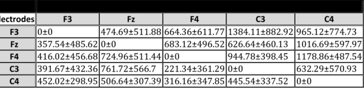
Indeed, this test must be used to assess the statistical significance of the Granger causality analysis results provided by PDC estimation. In particular, according to this test, all improper values that do not signify any right interaction between the electrodes are set to zero. Then the real connections between electrodes can be represented through graphs in which each node corresponds to an electrode.

2.2 Methods of Analysis

2.2.1 EEGLAB Matlab Toolbox

After the acquisition of the EEG raw signals from the scalp electrodes of the eight subjects, such data need to be further viewed and analyzed.

EEGLAB is a complete interactive environment toolbox for processing EEG data under Matlab, to provide both standard and advanced EEG processing functions. It allows reading of data, event information, and channel location files in several different formats including binary, Matlab, ASCII, Neuroscan, EGI, Snapmaster, European standard BDF, and Biosemi EDF (25). In general, it also allows the analysis of data by filtering, selecting and extracting epochs, removing baseline, and data re-sampling.

In this project, EEGLAB version 11 has been used for analyzing the raw EEG data. Experimentally, as the aim of this project was to analyze the EEG behavior and therefore connectivity throughout certain lobes, epochs were supposed to be extracted from each minute of the raw EEG signals. First of all, EEGLAB allowed us to load the 22 raw signals at first. Then, as seen in figure 6 below, all the raw signals are presented for each subject for ten continuous minutes, showing the 22 channels per frames and the sampling rate used.

Nontheless, signals from electrooculogram (EOG), electrocardiogram (ECG), electromiogram (EMG), which correspond to electrical activity of the eyes, heart and muscles respectively are also recorded; however they are disregarded in this study, because we are focusing on the brain signals only. For this reason, all the next elaborations will be done only on the 19 EEG signals. Figure 7below shows how to load a raw signal from a file menu as well as all the charactersiticsof the

(24)

15

signal itself including the epochs, events, data size, number of channels and the total duration of the recording.

Figure 6 Raw EEG signals recorded from 19 electrodes and ECG, EOG and EMG for one subject during 10 minutes. In the figure only 5 seconds are displayed.

Figure 7 Loading EEG ten-minutes recording of a subject into EEGLAB using MATLAB.

The following step was to apply a filter to the raw signals, in order to filter out all unwanted artifacts (especially power line noise at 50-60 Hz). The filter applied was a band-pass filter between 1 Hz and 48 Hzto remove noises and muscular artifacts. Moreover, the EEG data were down sampled at 100 Hz as shown in figure 8 below, in order to reduce the number of samples that should be analyzed.

(25)

16

Figure 8 Changing the sampling rate to 100 Hz of the ten-minutes recording of a subject in EEGLAB.

Each subject has two EEG raw data: ten-minutes recording while paying attention and reacting with a response to a certain visual stimulus one a computer screen, and two-minutes baseline recording while the subject is at rest with absence of any visual stimulus.

Figure 9Schematic representation of the procedure followed while extracting epochs in EEGLAB

As illustrated in figure 9 above; each minute of the total 12 minutes of EEG recording (Conners test + baseline) for each subject is divided into 10 epochs intervals of 1.2 seconds each; that results in a total of 100 epochs for the 10 minutes Conners test recording, and 20 epochs for the 2 minutes of baseline recording. Eventually, these epochs are stored in order to be further analyzed and spatial filtered using Laplace Transformation.

(26)

17

2.2.2 Laplace Transform

During complex tasks, the relationships between different cortical regions can be evaluated through the calculation of the squared coherence function between couples of electrodes. However, scalp recorded electrical potentials are influenced by volume conduction effects, that lead to spatial blurring attenuation, and by the reference chosen, that is not often an inactive electrode. Both these effects lead to an enhanced coherence among electrodes that do not reflect a real link among the underlying cortical areas (21).

A useful technique for improving spatial resolution and minimizing or eliminating conduction effects is the surface Laplacian transformation (L-transformation), which can be used as a spatial high-pass filter to better evidence the underlying local brain activity (26).

Moreover, Van Dijik et al. investigated the applications and physical interpretations of EEG surface Laplacian estimates, and they evaluated the surface Laplacian approach in the context of High Resolution EEG. The term " High Resolution EEG" refers to several approaches by which the spatial resolution on scalp recorded data is improved over conventional EEG. Such method involves a combination of high electrode density as well as advanced computer algorithms that "know" some important features of head volume conduction. These algorithms provide predictions of cortical surface potential distributions, which maybe can be far more accurate than those obtained from potentials recorded on the scalp (27) (28).

The raw EEG signals for the eight subjects (four subjects with TBI and four control subjects) are spatial filtered by using L- Transformation, thus their volume conduction effects on electrodes are reduced.

2.2.2.1 Spherical Splines Interpolation

In order to compute the Laplacian transformation, EEG potentials between the 19 electrode locations are estimated by calculating scalp spherical splines interpolations directly from the measured raw data. Spherical Splines Interpolation is the method used in this project. It assumes spherical head geometry.

(27)

18

The Spherical splines interpolation method assumer as the radius of the sphere that models the head, and 𝒓𝒓_𝒊𝒊is the location of the i-th of the 19 measurement electrodes. The Spherical Splines interpolation method assumes that the potential at any point r on the surface of the sphere can be represented by equation (1) below:

𝜇𝜇(𝑟𝑟⃗) = 𝑐𝑐0 + � 𝑐𝑐𝑖𝑖 𝑔𝑔𝑚𝑚 19

𝑖𝑖 = 1 (𝑐𝑐𝑐𝑐𝑐𝑐(𝑟𝑟, 𝑟𝑟𝑖𝑖)) (1)

Where𝑔𝑔_𝑚𝑚 (𝑥𝑥) is defined in equation (2) below:

𝑔𝑔(𝑥𝑥) = 1 4π � 2𝑘𝑘 + 1 𝑘𝑘𝑚𝑚−1_{(𝑘𝑘 + 1)}𝑚𝑚 ∞ 𝑘𝑘=1 𝑃𝑃𝑘𝑘(𝑥𝑥) (2)

The function 𝑃𝑃_𝑘𝑘(𝑥𝑥) is the Legendre polynomial of order k, which form a complete set of basis functions on a spherical surface assuming azimuthally symmetry. The parameter ris equals to 9 cm. The variable x in𝑃𝑃_𝑘𝑘(𝑥𝑥) represents the angle between the electrode position 𝒓𝒓_𝒊𝒊and the interpolation point r, thus this set of functions is capable of describing arbitrary scalp potentials. The procedure works by effectively treating each electrode as a field source located at the north pole, then rotating the coordinate system to account for the actual electrode position (29). Actually the constant m in 𝑔𝑔(𝑥𝑥) is called the “order” of the interpolation. For any m = 3, the function 𝑔𝑔𝑚𝑚(x) converges to an

almost exactly linear function of x. In other words, the spherical spline interpolation algorithm for m = 3 is essentially a linear interpolation algorithm, if the linear interpolation variable x is understood to be the cosine of the angle between each measurement electrode 𝒓𝒓_𝒊𝒊 andthe interpolation point r.

2.2.2.2 Laplace Transform Evaluation

The Laplacian C(E) in the E location of the scalp proportional to the radial current density is presented in equation (3) below:

(28)

19 𝐶𝐶(𝐸𝐸) = � 𝑐𝑐𝑖𝑖

𝑛𝑛 𝑖𝑖=1

. ℎ(𝑐𝑐𝑐𝑐𝑐𝑐(𝐸𝐸, 𝐸𝐸𝑖𝑖)) (3)

Where the radial current density is the quantity of the electrical current over a radial cross-sectional area. 𝑐𝑐𝑐𝑐𝑐𝑐(𝐸𝐸, 𝐸𝐸_𝑖𝑖)is the cosine of the angle between the electrode projections on the spherical surface, and h(x) is defined as:

ℎ(𝑥𝑥) =_{4π �}1 _𝑘𝑘_𝑚𝑚−12𝑘𝑘 + 1_{(𝑘𝑘 + 1)}_𝑚𝑚−1

∞ 𝑘𝑘=1

𝑃𝑃𝑘𝑘(𝑥𝑥) (4)

Where 𝑃𝑃_𝑘𝑘(𝑥𝑥) is the Legendre polynomial of order k, and the order is taken as k =20. Moreover, 𝑐𝑐_𝑖𝑖 coefficients are computed by solving the matrix equation system in equation (5) below:

�𝐺𝐺𝐶𝐶 + 𝑇𝑇𝑐𝑐0 = 𝑍𝑍

𝑇𝑇′ 𝑐𝑐 = 0 (5)

In the equation system, T = [1 1. . . . 1], C =�𝑐𝑐_{1 ,}𝑐𝑐₂. . . . 𝑐𝑐_𝑛𝑛,�and Z =�𝑧𝑧_{1 ,}𝑧𝑧₂. . . . 𝑧𝑧_𝑛𝑛,�is the vector of the potential values measured at the 19 electrodes, and G = g(cos(E, , 𝐸𝐸_𝑖𝑖) and g(x) is defined in

Equation (2).

A calculation procedure of L-Transformation of the raw EEG signals for 19 electrodes implemented in MATLAB language was used in this project to spatially filter the raw EEG data of each subject. Figure 10 below shows the raw EEG signal taken from electrode F3 of the first control subject. The duration of the epoch is 1.2 seconds, and the scale is between -25 𝜇𝜇𝜇𝜇 𝑡𝑡𝑐𝑐 20 𝜇𝜇𝜇𝜇.

(29)

20

Figure 10 Epoch sample of one subject, showing the raw EEG signal taken from electrode F3

Figure 11 below shows the same epoch sample taken from F3 electrode from the same control subject, however showing only the Laplace transform of the signal with a zoomed scale from -1.5 nV/m2_{to 1.5}_nV/m2_{duringthe 1.2 seconds.}

(30)

21

2.2.3Granger multivariate autoregressive connectivity

During the last decade, investigation of brain activity has put increasing emphasis on the analysis of causal interactions (the so-called effective connectivity) within networks of cerebral areas. Among the existing techniques to investigate effective connectivity, multivariate Granger Causality Analysis (GCA) was increasingly used to overcome the requirements of a priori hypothesis about the connectivity structure (3).

Effective connectivity, indeed, reveals the strength and the direction of the information flow between brain areas (Friston et al. 1993), and it can be addressed by GCA approach. This approach tries to estimate directed causal influences between cerebral structures by extracting useful information from the temporal dynamics of signals measuring directly or indirectly neuronal activity from different brain areas (3).

Over recent years there has been growing interest in the use of Granger Causality to identify causal interactions in neural data. Bernasconi (1999) applied spectral measures to describe causal interactions among different areas in the cat visual cortex. Liang et al. (2000) used a time-varying spectral technique to differentiate feed-forward, feedback, and lateral dynamical influences in visual cortex during pattern discrimination. Finally, Kaminski et al. (2001) noted increasing anterior to posterior causal influences during the transition from waking to sleep by analysis of EEG signals. Granger multivariate autoregressive connectivity (GMAC) is a Matlab toolbox (Tana et al 2012) that has been used in this project to study brain connectivity among the five selected electrodes. In particular it receives the EEG Laplace-transformed data as input, and applies Granger causality analysis to give information about brain connectivity among the before mentioned electrodes. The toolbox is an open source software provided with Graphical Users Interface (GUI); it is entirely developed in Matlab (The MathWorks Inc., Natick, MA, USA) environment and it works with the freely available BIOSIG toolbox (30)

Figure 12 below shows the different modules from the GMAC toolbox that have been used in the present project to perform the GCA analysis of the EEG data relative to the five selected electrodes, having already filtered and laplace-transfromed them in order to reduce the volume conduction from its surroundings. The first step was to consider the 5 EEG signals as an input in order to process them. This input is a bi-dimensional array (time points x 5 channels) for epochs of 1.2 seconds each in Matlab format (.mat). Then the signals are analyzed with Multivariate

(31)

22

Autoregressive (MVAR) modeling followed by granger causality estimation and graphical representation of the Partial Directed Coherence index (PDC).

Figure 12Block diagram of GMAC structure following the organization of the GMAC starting GUI and showing the three functional modules of the toolbox that have been used in the present project.

2.2.3.1 Preconditioning and MVAR modeling

The second module, that is the pre-conditioning phase, allows preconditioning the signal and the identification of the network nodes. The preconditioning follows the stationarity test, in which each time series is evaluated for covariance stationarity (Seth et al. 2010). This test verifies if the statistical moments of the first and second order do not change throughout time in the considered epoch. As a consequence, large values will be followed by smaller values, and small values by larger values. Then MVAR modeling is applied to the 5-channel data, the optimum order found for all the epochs in the present project wasp=2. Equation (6) below shows the MVAR model:

𝑌𝑌(𝑡𝑡) = � 𝐴𝐴(𝑖𝑖) (𝑡𝑡 − 1) + 𝐸𝐸(𝑡𝑡) (6)

𝑝𝑝 𝑖𝑖=1

Where A(i) are the model parameters and E(t) is the vector representing the white noise process. One criterion implemented in the software in order to find the optimum order of the MVAR models the Multivariate Bayesian Information Criterion (BIC), and it is represented in equation (7) below:

(32)

23

Where T is the number of data time points, m is the number of channel and S denotes the noise covariance matrix.

Figure 13 below shows how a sample epoch (bi-dimensional array: time points x 5 channels) is imported into the GMAC Matlab toolbox, preconditioned and treated through MVAR Modeling. The parameter TR = 0.01 seconds corresponds to the inverse of the sampling rate of 100 Hz, and the frequency range has been put automatically according to the imported data (having a sampling rate of 100 Hz, the Nyquist frequency is 50 Hz).

Figure 13 GMAC starting GUI running under MaC OS X 10.6 operating system. Data is imported and functions for subGUIs for the GCA analysis are called by means of pushbuttons located on GMAC starting interface.

Figure 14 below shows the MVAR estimation using the BIC criterion for the identification of the optimum order necessary for the same epoch of the five electrodes of a subject randomly chosen among the 8 considered.

(33)

24

Figure 14 Screenshot of the choice of the optimum order from BIC criterion, using GMAC Matlab toolbox running under MaC OS X 10.6 operating system.

2.2.3.2 Partial Directed Coherence

Partial Directed Coherence (PDC) is a spectral index that can tell whether and how two structures under study are functionally connected. PDC estimation requires the reliable fitting of MVAR models, which is treated in depth elsewhere (31). Moreover, are liable structure interference depends heavily on the issue of statistical significance (rejecting interactions absence) through PDC estimation (Kaminsku et al. 1997), and it portrays the relative strength of direct pair wise structure interactions (32).

PDC takes values from the interval [0,1] and it shows only direct flows between channels. Equation (7) below shows the partial directed coherence as was defined by Baccala et al:

𝑃𝑃𝑖𝑖𝑖𝑖(𝑓𝑓) = 𝐴𝐴𝑖𝑖𝑖𝑖 (𝑓𝑓)

�𝑎𝑎𝑖𝑖∗(𝑓𝑓) 𝑎𝑎𝑖𝑖 (𝑓𝑓)

(𝑓𝑓) (7)

Where 𝐴𝐴_{𝑖𝑖𝑖𝑖}(𝑓𝑓) is an element of the matrix A(f) (a Fourier transform of MVAR model coefficients

A(t)). Moreover, 𝑎𝑎_𝑖𝑖(𝑓𝑓) represents the j-th column of A(f). PDC is normalized to show a ratio

(34)

25

In the present project, after the five-electrodes data epochs for each subject have been preconditioned and analyzed with MVAR of an optimum order equals to 2, the further data are elaborated through the third module, in which granger causality indexes estimation is performed. The sub GUI contains the push-button of the "Granger Causality Estimation", which is devoted to the calculation of the GCA spectral quantities (PDC) using Matlab functions. The output is the frequency course of the PDC values, and it plots the sum of these values over the range of frequency selected to form the adjacency matrix. Figure 15 shows the PDC adjacency matrix calculated on the sample data set for one epoch of 1.2 seconds for a subject randomly chosen among the 8 considered. In such graphical representation, the colors indicate the interactions strength (i.e., PDC value) normalized with respect to the maximum in the adjacency matrix. The directions of influence are from the columns to the rows (i.e., the matrix element(i,j) represents the strength of the connection from j-th node to the i-th node).

Figure 15 Adjacency Matrix showing the PDC Index after the granger causality estimation for a sample data epoch for a randomly chosen subject. The color map range from 0 to 1 corresponds to the strength of the connectivity between

(35)

26

Chapter 3 Results

The subjects were divided into two groups: Four TBI patients and four control subjects. In fact, in order to investigate the differences between the two groups, each group has been analyzed separately. The Partial Directed Coherence (PDC) was calculated for each epoch of each subject (in total 120 epochs of 1,2 seconds each), both for the Conners Test (CPT) ten minutes recordings and for the two minutes baseline recordings. The PDC values representing the strength of the interaction between the selected electrodes (nodes of the network)were estimated using Granger causality index through GMAC Matlab toolbox.

Moreover, the PDC values computed for each minute of each subject have been averaged. Thus, each subject will have: a total of 10 PDC mean 5x5 adjacency matrices(representing the 10 minutes of the main CPT recording), and two PDC mean 5x5 adjacency matrices(representing the two minutes baseline recording).

For a better investigation of the achieved results, the mean PDC estimations have been also averaged to mean values for both groups (four TBI patients and four controls), having at the end: ten mean PDC 5x5 adjacency matrices (representing the 10 minutes of the main CPT recording), and one mean PDC 5x5 adjacency matrices(representing the two minutes baseline recording). These adjacency matrices are presented in the following subsections as results.

3.1 Mean PDC Estimates for Control Subjects

The mean PDC values obtained for the 4 healthy volunteers participating in the study are represented below in the 5x5 adjacency matrices. In particular, ten mean PDC 5x5 adjacency matrices (representing the 10 minutes of the main CPT recording), and one mean PDC 5x5 adjacency matrices (representing the two minutes baseline recording) are reported (Tables 1-11).

(36)

27

Each 5x5 table below represents the overall mean PDC estimations for each minute of the control group. These estimations represent the strength of interactions between the following nodes or electrodes: • F3 = node 1 • Fz= node 2 • F4 = node 3 • C3= node 4 • C4= node 5

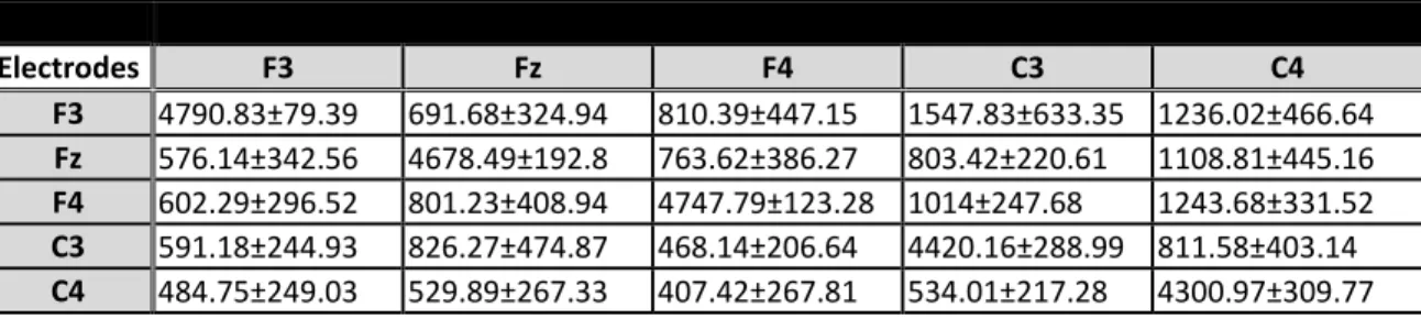
Table 1 : Mean PDC values of the 1st _{min calculated using MATLAB at the 5}

selected nodes for the normal subjects group.

1st min Mean PDC Electrodes F3 Fz F4 C3 C4 F3 4790.83±79.39 691.68±324.94 810.39±447.15 1547.83±633.35 1236.02±466.64 Fz 576.14±342.56 4678.49±192.8 763.62±386.27 803.42±220.61 1108.81±445.16 F4 602.29±296.52 801.23±408.94 4747.79±123.28 1014±247.68 1243.68±331.52 C3 591.18±244.93 826.27±474.87 468.14±206.64 4420.16±288.99 811.58±403.14 C4 484.75±249.03 529.89±267.33 407.42±267.81 534.01±217.28 4300.97±309.77

Table 2 : Mean PDC values of the 2nd _{min calculated using MATLAB at the 5}

2nd min Mean PDC Electrodes F3 Fz F4 C3 C4 F3 4791.3±84.6 821.87±427.53 968.19±533.03 787.22±461.36 1225.09±412.2 Fz 633.74±281.58 4713.92±159.54 514.9±238.38 882.65±626.58 804.14±379.48 F4 614.12±228.56 452.16±205.29 4648.94±248.73 898.07±482.26 1020.54±411.99 C3 611.7±309.4 660.88±461.54 573.58±342.37 4623.27±221.53 890.34±296.89 C4 416.62±200.59 632.11±361.78 596.25±365.56 412.92±340.16 4430.6±196.58

Table 3 : Mean PDC values of the 3rd _{min calculated using MATLAB at the 5}

3rd_min _{Mean PDC} Electrodes F3 Fz F4 C3 C4 F3 4822.12±70.44 575.89±323.33 717.59±464.44 908.53±500.16 842.28±557.19 Fz 674.63±184.53 4789.25±89.99 594.24±195.47 608.16±257.13 1233.31±407.67 F4 500.56±151.68 524.62±333.78 4736.78±126.18 935.28±504.44 854.52±422.8 C3 713.21±316.58 727.47±207.23 568.5±191.34 4663.65±219.75 626.7±464.07 C4 310.53±177.81 467.5±275.29 559.17±298.97 492.82±327.83 4513.46±335.37

(37)

28

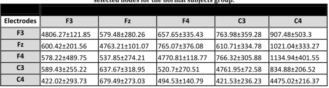
Table 4 : Mean PDC values of the 4th _{min calculated using MATLAB at the 5}

4th_min Mean PDC Electrodes F3 Fz F4 C3 C4 F3 _{4806.27±121.85 579.48±280.26} _{657.65±335.43} _{763.98±359.28 907.48±503.3} Fz _{600.42±201.56} _{4763.21±101.07 765.07±376.08} _{610.71±334.78 1021.04±333.27} F4 _{578.22±489.75} _{537.85±274.21} _{4770.81±118.77 766.32±305.88 1134.94±401.55} C3 _{589.43±255.22} _{637.67±318.95} _{520.7±270.51} _{4761.95±72.58 834.88±206.52} C4 _{422.02±293.73} _{679.49±273.03} _{494.53±140.79} _{421.53±236.23 4475.02±216.37}

5th_min _{Mean PDC} Electrodes F3 Fz F4 C3 C4 F3 4700.4±143.61 827.62±353.8 902.6±591.92 975.33±323.02 1420.48±790.68 Fz 619.74±248.17 4615.73±166.31 719.98±328.64 576.78±223.07 894.42±477.41 F4 862.91±522.61 651.27±301.19 4619.03±285.16 832.22±300.27 1266.94±476.12 C3 769.23±267 855.5±235.03 646.91±478.04 4708.98±90.54 505.39±254.58 C4 623.87±311.08 767.46±257.25 536.35±307.2 490.13±237.04 4243.12±458.34

Table 6 : Mean PDC values of the 6th_{min calculated using MATLAB at the 5}

6th_min _{Mean PDC} Electrodes F3 Fz F4 C3 C4 F3 4792.99±75.2 763.69±351.46 640.82±351.82 674.79±396.5 1288.55±477.75 Fz 614.43±224.1 4716.32±173.73 565.3±244.05 635.46±351.17 749.98±418.01 F4 775.25±321.83 641.14±373.42 4749.13±116.58 1115.16±372.89 989.35±492.82 C3 522.66±311.53 701.21±434.99 788.05±252.57 4652.27±126.93 1030.88±474.58 C4 411.81±166.19 459.47±265.51 464.81±265.52 679.34±319.98 4360.48±185.48

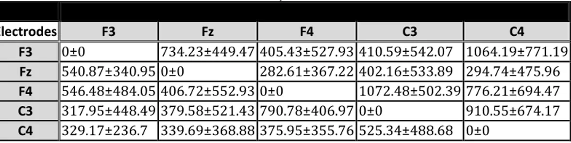
7th_min _{Mean PDC} Electrodes F3 Fz F4 C3 C4 F3 4775.46±87.69 659.9±424.67 743.73±248.04 854.45±287 808.81±265.61 Fz 747.81±294.4 4717.39±141.18 625.42±321.38 946.27±497.74 1085.1±319.78 F4 668.23±206.88 617.55±185.29 4738.06±103.71 833.44±496.18 1025.92±410.41 C3 601.91±354.84 618.37±413.03 558.14±337.09 4632.88±168.91 924.92±330.39 C4 490.3±297.91 554.89±383.54 671.83±320.33 575.55±185.5 4504±160.46

8th min Mean PDC Electrodes F3 Fz F4 C3 C4 F3 4804.96±79.43 769.36±420.15 763.43±462.58 934.77±305.92 1166.71±491.78 Fz 628.59±286.6 4732.87±138.45 622.35±400.26 693.12±551.66 971.2±384.66 F4 713.81±296.44 510.44±218.94 4739.5±145.05 932.16±362.44 1170.99±575.42 C3 521.78±308.7 766.89±339.33 594.25±186.39 4652.04±108.22 716.98±405.84 C4 436.29±140.97 463.57±266.6 461.86±205.69 503.17±251.53 4401.86±251.81