AC corrosion of carbon steel in cathodic protection condition: effect on potential and confirmation of protection criteria

POLITECNICO DI MILANO

School of Industrial and Information Engineering

Department of Chemistry, Materials and Chemical Engineering “Giulio Natta”

Master of Science in Materials Engineering and Nanotechnology

AC CORROSION OF CARBON STEEL IN

CATHODIC PROTECTION CONDITION: EFFECT

ON POTENTIAL AND CONFIRMATION OF

PROTECTION CRITERIA

Supervisor:

Prof. Marco ORMELLESE

Co-Supervisor: Ing. Andrea BRENNA

Master Thesis of:

Francesco LIPARI

Matr.: 854228

Content

CHAPTER 1 -AC INTERFERENCE CORROSION OF CARBON STEEL ... 1

1.1 CATHODIC PROTECTION: GENERAL [4] ... 1

1.1.1 Cathodic protection systems ... 2

1.1.2 Protection potential ... 3

1.1.3 Protection current density ... 6

1.1.4 Cathodic protection criteria ... 7

1.2 AC INTERFERENCE ... 8

1.2.1 Stationary and non-stationary interference ... 9

1.2.2 AC interference sources... 11

1.2.2 Capacitive coupling ... 12

1.2.3 Resistive coupling ... 12

1.2.4 Inductive coupling ... 13

1.3 CHARACTERISTICS OF AC CORROSION ... 14

1.3.1 AC voltage on the structure ... 14

1.3.2 AC density ... 15

1.3.3 AC density/DC density ratio ... 16

1.3.4 Effect of polarization potential ... 16

1.3.5 Soil characteristics ... 17

1.3.6 Frequency effect ... 19

1.3.7 Corrosion Rate ... 20

1.3.8 Morphology of AC corrosion ... 21

1.4 AC CORROSION MONITORING... 22

1.4.1 Weight loss measurements ... 24

1.4.3 Electrical resistance (ER) measurements ... 25

1.4.4 Coulometric oxidation of corrosion product measurements ... 25

1.5 AC MITIGATION ... 26

1.5.1 Construction measures ... 26

1.5.2 Operation measures ... 27

CHAPTER 2 - AC CORROSION: PROPOSED MECHANISMS AND PROTECTION CRITERIA ... 28

2.1 AC CORROSION MECHANISMS ... 28

2.1.1 The mechanism reported on ISO 18086:2015 ... 28

2.1.2 Analysis of equivalent electric circuits ... 30

2.1.3 Earth-alkaline vs. alkaline cations effect ... 35

2.1.4 A conventional electrochemical approach in the absence of CP ... 36

2.1.5 The alkalization mechanism ... 38

2.1.6 Theoretical corrosion models ... 41

2.1.7 AC effect on overvoltages ... 45

2.1.8 A two-steps mechanism ... 47

2.2 CATHODIC PROTECTION CRITERIA ... 50

2.2.1 Cathodic protection criteria reported on ISO 18086:2015 ... 50

2.2.2 Cathodic protection criteria proposed by other authors... 52

2.2.3 A new proposal of CP criteria in the presence of AC interference ... 54

CHAPTER 3 - MATERIALS AND METHODS ... 58

3.1 ELECTRICAL CIRCUIT... 58

3.2 MATERIALS ... 60

3.3 GALVANOSTATIC TEST: AC EFFECT ON DC POTENTIAL ... 61

3.3.1 Aim of the test ... 61

3.3.2 Electrical circuit and test cell... 63

3.4.1 Aim of the test ... 64

3.4.2 Electrical circuit and test cell... 65

3.4.3 Protection potential and current density monitoring ... 67

3.4.4 Mass loss measurement ... 68

CHAPTER 4 - RESULTS AND DISCUSSION ... 70

4.1 PART 1: GALVANOTATIC TESTS: EFFECT OF AC ON IR-FREE POTENTIAL ... 70

4.2 PART 2: LONG-TERM EXPOSURE TEST: CURRENT AND POTENTIAL MONITORING ... 81

4.3 PART 3: LONG-TERM EXPOSURE TEST: CORROSION RATE AND CATHODIC PROTECTION CRITERIA ... 88

4.3.1 Corrosion rate in the presence of AC interference ... 88

4.3.2 Cathodic protection criterion in the presence of AC interference ... 93

CONCLUSIONS ... 101

1 GALVANOTATIC TESTS: EFFECT OF AC ON IR-FREE POTENTIAL ... 101

2 LONG-TERM EXPOSURE TESTS FOR MASS LOSS MEASUREMENT .... 102

List of figures

Figure 1.1 Types of cathodic protection: a) by galvanic anodes b) by impressed current system [4] _{... 2}

Figure 1.2 Schematic illustration of the electrochemical mechanism [5] ... 5

Figure 1.3 a) A generic Evans diagram and b) Evans diagram for an active metal

in aerated environment, as carbon steel in soil [4] _{... 5}

Figure 1.4 General scheme of electrical interference between two electrodes on a body: a) conductor and b) insulator [4] ... 9

Figure 1.5 Scheme of stationary interference between: a) two crossing pipelines and b) two almost parallel pipelines [4] ... 9

Figure 1.6 Scheme of non-stationary interference caused by stray current

dispersed by a DC transit system [4] ... 10

Figure 1.7 An example of HVTL ... 12

Figure 1.8 A Frecciarossa 1000 (ETR 1000) on an Italian high-speed railway [12] ... 12

Figure 1.9 Inductive coupling between an AC conductor and a buried pipeline [15] . 13

Figure 1.10 Inductive coupling between three-phases HVTL and a buried

pipeline [15] ... 13

Figure 1.11 AV needed to have a 𝑖_𝐴𝐶 of 100 A/m2, in function of the defect

diameter and the soil resistivity [20] ... 17

Figure 1.12 Electric equivalent circuit [33] ... 19

Figure 1.13 Electrical response of the circuit in Figure 1.12: the red line is the

total AC, the green line is the AC passing through 𝑅_𝑒𝑓𝑓[33] _{... 20}

Figure 1.14 Schematic illustration of the tubercle of “stone hard soil” that grows

at the coating defect in connection with AC corrosion [36] ... 22

Figure 1.15 Measurement of the AC gradient and localising remote earth [16] ... 24

Figure 2.1 Schematic description of the AC corrosion process with cathodic protection according to ISO 18086, where: 1) AC current on a

coating defect, 2) metal, 3) passive film and 4) iron hydroxide [16] _{... 29}

Figure 2.2 A schematic illustration of the electrical equivalent circuit [36] ... 31

Figure 2.3 Geometrical effects on pipe-to-soil resistance [36] ... 31

Figure 2.4 Illustration of the anodic- and cathodic branches of the

Volmer-Butler equation and the summarised total current [36] ... 33

Figure 2.5 Schematic illustration of the steel-water interface acting as a

Figure 2.6 An electrochemical description of AC corrosion [33] ... 37

Figure 2.7 An electrochemical description of AC corrosion [33] ... 38

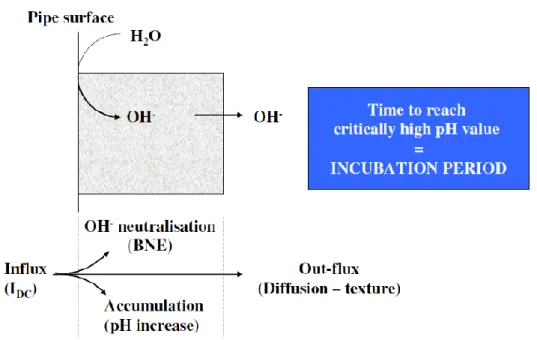
Figure 2.8 Mass balance schematics for 𝑂𝐻− _{ions produced by CP at a coating} defect [42] ... 39

Figure 2.9 Pourbaix diagram: the hatched area indicates the critical AC corrosion zone [42] _{... 39}

Figure 2.10 DC on-potential (𝑈_𝑂𝑁) and corrosion rate measured with ER coupon [42] ... 40

Figure 2.11 DC on-potential (𝑈_𝑂𝑁) and spread resistance (𝑅_𝑆) measured with ER coupon [42] ... 41

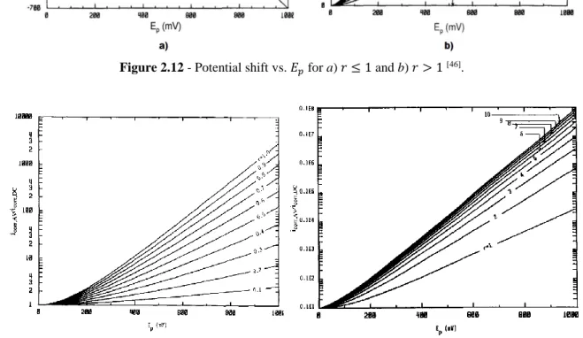
Figure 2.12 Potential shift vs. 𝐸𝑝 for a) 𝑟 ≤ 1 and b) 𝑟 > 1 [46] ... 43

Figure 2.13 Corrosion current vs. 𝐸𝑝 for a) 𝑟 ≤ 1 and b) 𝑟 > 1 [46] ... 43

Figure 2.14 DC potential vs the root-mean-square current for a) 𝑟 < 1 and b) 𝑟 > 1 [47] _{... 43}

Figure 2.15 𝐸𝑟.𝑚.𝑠.,min vs r [47] ... 44

Figure 2.16 𝑖𝑟.𝑚.𝑠.,min vs r [47] ... 44

Figure 2.17 Electrical equivalent circuit proposed by Lalvani and Xiao [48]... 45

Figure 2.18 Dimensionless corrosion current vs a) peak potential and b) frequency [48] ... 45

Figure 2.19 ∆𝐸𝑐𝑜𝑟𝑟 vs 𝐸𝑝[48] ... 45

Figure 2.20 Dimensionless corrosion current vs 𝐸_{𝑐𝑜𝑟𝑟}[48] _{... 45}

Figure 2.21 Effect of AC on polarisation curves of carbon steel in 4 g/L 𝑁𝑎2𝑆𝑂4 solution [49] ... 46

Figure 2.22 Effect of AC on corrosion current and potential for carbon steel in 4 g/L 𝑁𝑎₂𝑆𝑂₄ solution [49] ... 47

Figure 2.23 Relationship between DC on-potential, AC voltage and likelihood of AC corrosion, where: 1) less negative cathodic protection level; 2) more negative cathodic protection level; 3) AC corrosion [16] ... 51

Figure 2.24 Relationship between DC and AC current densities and likelihood of AC corrosion, where: 1) less negative cathodic protection level; 2) more negative cathodic protection level; 3) AC corrosion [16] ... 52

Figure 2.25 Effect of soil resistivity on the threshold 𝑈_𝐴𝑉 value [54] ... 53

Figure 2.26 New CP criteria for mild pipeline steel in the present of AC interference for a) Tang et al. [56] and b) A.Q. Fu [57] ... 54

Figure 2.27 Experimental corrosion rate in the 𝑖𝐴𝐶/𝑖𝐶𝑃 diagram. Safe and unsafe regions refer to CP criterion as reported in ISO 18086:2015 [58] ... 55

Figure 2.29 New CP criteria based on experimental corrosion rate data [58] ... 57

Figure 3.1 Schematic view of the electrical circuit ... 59

Figure 3.2 Electrical circuit (case and internal view) ... 60

Figure 3.3 Carbon steel specimen in the sample holder ... 61

Figure 3.4 Galvanostatic test – experimental set-up ... 62

Figure 3.5 Galvanostatic test – electrochemical cell ... 62

Figure 3.6 Long-term exposure tests – experimental conditions (red markers refers to the first condition investigated; blue markers to the second condition) ... 65

Figure 3.7 Long-term exposure tests – schematic view of the electrical circuit ... 66

Figure 3.8 Long-term exposure tests – electrical circuit ... 66

Figure 3.9 Long-term exposure tests – connection between the electrical circuit and the corrosion cells ... 67

Figure 3.10 Long-term exposure tests – test cells ... 67

Figure 3.11 IR-free potential monitoring ... 68

Figure 4.1 DC potential vs. AC density (𝑖𝐶𝑃 = 0 A/m2) ... 72

Figure 4.2 DC potential vs. AC density (𝑖_𝐶𝑃 = 0.15 A/m2) ... 72

Figure 4.3 DC potential vs. AC density (𝑖_𝐶𝑃 = 0.3 A/m2) ... 72

Figure 4.4 DC potential vs. AC density (𝑖_𝐶𝑃 = 0.5 A/m2) ... 72

Figure 4.5 DC potential vs. AC density (𝑖_𝐶𝑃 = 1.0 A/m2) ... 73

Figure 4.6 DC potential vs. AC density (𝑖_𝐶𝑃 = 2.0 A/m2) ... 73

Figure 4.7 DC potential vs. AC density (𝑖_𝐶𝑃 = 3.0 A/m2) ... 73

Figure 4.8 DC potential vs. AC density (𝑖_𝐶𝑃 = 5.0 A/m2) ... 73

Figure 4.9 DC potential vs. AC density (𝑖_𝐶𝑃 = 10.0 A/m2) ... 73

Figure 4.10 IR-free potential vs 𝑖_𝐶𝑃 in absence of interference 𝑖_𝐴𝐶 (𝑖_𝐶𝑃 from 0 to 10 A/m2) ... 77

Figure 4.11 IR-free potential vs. AC density varying CP current density (𝑖_𝐶𝑃 from 0.15 to 1 A/m2) ... 77

Figure 4.12 IR-free potential vs. AC density varying CP current density (𝑖𝐶𝑃 from 2 to 10 A/m2) ... 78

Figure 4.14 Protection potential shift vs AC density (comparison between the

results obtained in this work and in [58]) ... 80

Figure 4.15 IR-free potential monitoring in time (Series A and B) ... 83

Figure 4.16 IR-free potential monitoring in time (Series A and B) ... 83

Figure 4.17 Cathodic protection current density monitoring ... 84

Figure 4.18 AC density monitoring ... 84

Figure 4.19 𝑖_𝐴𝐶/𝑖_𝐶𝑃 ratio trend in time ... 85

Figure 4.20 Potentials obtained during the two testes at 𝑖_𝐶𝑃 = 0.3 A/m2 ... 86

Figure 4.21 Potentials obtained during the two testes at 𝑖_𝐶𝑃 = 0.5 A/m2 ... 86

Figure 4.22 Potentials obtained during the two testes at 𝑖_𝐶𝑃 = 1.0 A/m2 ... 86

Figure 4.23 Potentials obtained during the two testes at 𝑖_𝐶𝑃 = 2.0 A/m2 ... 86

Figure 4.24 Potentials obtained during the two testes at 𝑖_𝐶𝑃 = 10.0 A/m2 ... 87

Figure 4.25 Corrosion rate vs 𝑖_𝐴𝐶 at different CP levels. Blue markers refer to the tests carried out during this thesis work. White markers refer to results obtained from previous tests ... 90

Figure 4.26 Corrosion rate vs 𝑖_𝐴𝐶/𝑖_𝐶𝑃 at different AC and CP levels. Blue markers refer to the tests carried out during this thesis work. White markers refer to results obtained from previous tests ... 91

Figure 4.27 IR-free potential with respect to the ratio between AC and CP current density. Blue markers refer to the tests carried out during this thesis work. White markers refer to results obtained from previous tests ... 92

Figure 4.28 Relationship between DC and AC current densities and likelihood of AC corrosion, where: 1) less negative cathodic protection level; 2) more negative cathodic protection level; 3) AC corrosion [16] ... 94

Figure 4.29 Corrosion rates of carbon steel specimen under CP condition in the presence of AC interference: 𝑖𝐴𝐶 vs 𝑖𝐶𝑃 graph ... 95

Figure 4.30 Experimental corrosion rate in the 𝑖𝐴𝐶/𝑖𝐶𝑃 diagram. Safe and unsafe regions refer to CP criterion as reported in ISO 18086:2015 ... 96

Figure 4.31 Experimental corrosion rate in the 𝑖_𝐴𝐶/𝑖_𝐶𝑃 vs IR-free potential diagram. Safe and unsafe regions refer to CP criterion as reported in ISO 18086:2015 ... 97

Figure 4.32 Experimental corrosion rate in the 𝑖_𝐴𝐶 vs IR-free potential diagram. Safe and unsafe regions refer to CP criterion as reported in ISO 18086:2015 ... 98

Figure 4.33 Experimental corrosion rate in the 𝑖_𝐴𝐶 vs IR-free potential diagram. Safe and unsafe regions refer to CP criterion as reported in [58] ... 98

List of tables

Table 1.1 Protection potentials for different metallic materials and environmental conditions ... 8

Table 3.1 API 5L X52 – chemical composition by weight [59] _{... 60}

Table 3.2 Galvanostatic test – experimental conditions ... 63

Table 3.3 Long-term exposure tests – experimental conditions (according to Figure 3.6) ... 64

Table 4.1 (a) IR-free potential shift in the presence of AC interference (𝑖_𝐴𝐶 from 0 to 30 A/m2)... 74

Table 4.1 (b) IR-free potential shift in the presence of AC interference (𝑖𝐴𝐶 from

50 to 500 A/m2)... 75

Table 4.1 (c) IR-free potential shift in the presence of AC interference

(𝑖_𝐴𝐶 = 1,000 A/m2) ... 76

Table 4.2 IR-free potential of carbon steel in free corrosion condition in the

presence of AC interference ... 76

Table 4.3 IR-free potential after two weeks of cathodic protection applied ... 81

Table 4.4 Mean values of IR-free potential and current densities in the first

tested conditions ... 85

Table 4.5 Mean values of IR-free potential and current densities in the second tested conditions ... 85

Table 4.6 IR-free potential and potential shift in the first period of long-exposure test (from AC application to current variations). IR- free potential is expressed in V versus CSE ... 87

Table 4.7 IR-free potential and potential shift in the second period of long-exposure test (from current variations to the end of the test).

IR- free potential is expressed in V versus CSE ... 88

Table 4.8 Corrosion rate due to AC interference on cathodically protected carbon steel ... 89

Sommario

Le strutture metalliche interrate, come ad esempio le condotte d’acciaio per il trasporto di idrocarburi, sono protette dalla corrosione esterna mediante un sistema di protezione catodica combinato all’utilizzo di rivestimenti. La protezione catodica è una tecnica consolidata che consente di annullare o minimizzare la corrosione del metallo mediante l’applicazione di una corrente (catodica appunto) che polarizza il metallo al di sotto del cosiddetto potenziale di protezione, -0.85 V CSE per l’acciaio al carbonio in ambiente aerato. Tuttavia, la presenza di interferenza elettrica da corrente alternata non esclude la corrosione in corrispondenza dei difetti dei rivestimenti, anche se il criterio di protezione è correttamente rispettato. La corrosione da corrente alternata necessita di una sorgente di alimentazione, tipicamente gli elettrodotti e le linee ferroviarie alta velocità/alta capacità alimentate in corrente alternata a 50 Hz di frequenza. L’interferenza tra la linea interferente e la tubazione avviene con un meccanismo induttivo o conduttivo. La pericolosità sta nel fatto che la velocità di corrosione in corrispondenza dei difetti dei rivestimenti può essere molto elevata, dell’ordine di qualche mm/anno.

Tuttavia, nonostante sia un argomento discusso da decenni, il meccanismo di corrosione non è mai stato pienamente chiarito e, in secondo luogo, ci sono pareri discordanti sui criteri di protezione da adottare in presenza di interferenza. A livello normativo, esiste uno standard internazionale (ISO 18086) che definisce le soglie massima di accettabilità dell’interferenza in presenza di protezione catodica ma su queste soglie non c’è pieno accordo in ambito scientifico.

Il lavoro di tesi è parte di una ricerca in corso da oltre un decennio presso il Laboratorio di Corrosione dei Materiali “Pietro Pedeferri” del Dipartimento di Chimica, Materiali e Ingegneria Chimica "Giulio Natta" del Politecnico di Milano. Scopo della ricerca è studiare gli effetti della corrente alternata sulla corrosione dei metalli, in particolare sull’acciaio al carbonio in condizioni di protezione catodica. In questo contento, sono stati studiati gli effetti della corrente alternata sulla cinetica di corrosione, i criteri di protezione catodica da adottare in presenza di interferenza e il meccanismo di corrosione.

La tesi in particolare ha lo scopo di validare alcuni risultati ottenuti in passato in riferimento a due aspetti: 1) effetto della corrente alternata sul potenziale di protezione; 2) studio e

proposta di un criterio di protezione catodica in presenza di interferenza da corrente alternata.

La prima parte della tesi (Capitolo 1 e Capitolo 2) è incentrata sugli aspetti generali del fenomeno e sull’aggiornamento delle proposte riguardanti il meccanismo di corrosione presenti in letteratura. In particolare, in questa sezione sono riportati e descritti in senso critico i parametri considerati influenti per la corrosione da corrente alternata, così come riportati sullo standard ISO 18086. I parametri più importanti sono la tensione alternata indotta, la densità di CA, la densità di corrente di protezione, il potenziale di protezione, il rapporto tra la densità di CA e di protezione, le caratteristiche del suolo, la frequenza del segnale alternato. Ogni parametro è discusso in senso critico.

Nel Capitolo 2 sono descritti i principali modelli di meccanismo di corrosione dell’acciaio in protezione catodica in presenza di CA. È stato effettuato uno studio bibliografico che ha consentito di individuare i modelli più accreditati in ambito scientifico. In questa sezione è anche descritto brevemente il meccanismo di corrosione proposto che tuttavia non è stato oggetto della tesi.

Nel dettaglio, scopo delle prove effettuare è validare il criterio di protezione proposto in passato all’interno del filone di ricerca e parallelamente confrontarlo con il criterio proposto nello standard vigente ISO 18086. In breve, il criterio di protezione vigente limita il valore massimo della tensione alternata (misurata in posizione remota) a 15 V. In aggiunta, il criterio riporta il valore massimo di densità di corrente alternata accettabile in base al valore di densità di corrente continua (di protezione) e del potenziale ON. Nello specifico, per livelli di protezione catodica “più negativi” (𝐸_𝑜𝑛 < −1.2 V CSE) si ha:

 𝑉𝐶𝐴 |𝐸𝑂𝑁|−1.2< 3;  𝑖_𝐶𝐴 < 30 𝐴/𝑚2_;  𝑖𝐶𝐴 𝑖𝑃𝐶 < 3 se 𝑖𝐶𝐴 > 30 𝐴/𝑚 2_;

mentre, per livelli di protezione catodica “meno negativi” (−1.2 < 𝐸_𝑂𝑁 < −0.85 V CSE):  𝑉_𝐶𝐴 < 15 𝑉;

 𝑖𝐶𝐴 < 30 𝐴/𝑚2;

 𝑖_𝑃𝐶 < 1 𝐴/𝑚2 _{if 𝑖}

𝐶𝐴 > 30 𝐴/𝑚2.

Per validare questo criterio, fermo restando la validità dei 15 V alternati, sono state effettuate prove galvanostatiche in soluzione simulante terreno su provini di acciaio al carbono esposti a diversi valori di densità di corrente alternata e densità di corrente continua. Sono state

monitorate otto condizioni di protezione/interferenza: 1) 𝑖_𝐶𝐴 = 10 A/m2, 𝑖_𝐷𝐶 = 10 A/m2; 2) 𝑖𝐶𝐴 = 10 A/m2, 𝑖𝐷𝐶 = 1 A/m2; 3) 𝑖𝐶𝐴 = 30 A/m2, 𝑖𝐷𝐶 = 1 A/m2; 4) 𝑖𝐶𝐴 = 30 A/m2, 𝑖𝐷𝐶 = 0.2

A/m2; 5) 𝑖_𝐶𝐴 = 20 A/m2, 𝑖_𝐷𝐶 = 10 A/m2; 6) 𝑖_𝐶𝐴 = 20 A/m2, 𝑖_𝐷𝐶 = 2 A/m2; 7) 𝑖_𝐶𝐴 = 50 A/m2, 𝑖_𝐷𝐶 = 0.5 A/m2; 8) 𝑖_𝐶𝐴= 50 A/m2, 𝑖_𝐷𝐶 = 0.2 A/m2.

In sintesi, lo spettro di valori di densità di corrente alternata va da 10 a 50 A/m2 e quello della densità di corrente continua da 0.2 a 10 A/m2 (sovra protezione catodica). Questi valori sono stati scelti per completare le prove condotte in passato e per avere dati sensibili per il confronto con il criterio da normativa.

Le prove, della durata di tre mesi, sono state effettuate su provini da 1 cm2 simulanti un difetto del rivestimento di una tubazione protetta catodicamente e interferita. Le due correnti sono state applicate mediante un apposito circuito elettrico messo a punto nelle precedenti fasi della ricerca. Durante la prova, le densità di corrente alternata e continua e il potenziale dei provini sono stati monitorati. Al termine della prova la corrosione è stata valutata mediante misura di perdita di massa. A valle delle prove è proposto il seguente criterio di protezione, più restrittivo di quello riportato sullo standard ISO 18086, basato sul valore massimo accettabile di densità di corrente alternata:

 𝑖_𝐶𝐴 < 30 𝐴/𝑚2 _{se 𝑖}

𝑃𝐶 < 1 𝐴/𝑚2;

 𝑖_𝐶𝐴 < 10 𝐴/𝑚2 se 𝑖_𝑃𝐶 > 1 𝐴/𝑚2.

In altre parole, sono state misurate velocità di corrosione non trascurabili, ossia maggiori di 10 µm/anno, su provini che non si sarebbero dovuti corrodere secondo il criterio di protezione presente nella ISO 18086.

Un secondo set di prove è stato effettuato su provini della stessa tipologia applicando un valore di corrente di protezione costante e aumentando nel tempo la densità di corrente continua interferente. Scopo di queste prove non è misurare la velocità di corrosione ma studiare gli effetti sul potenziale IR-free, che in campo è la grandezza più importante e facile da misurare. Le prove sono state confrontate con alcuni risultati condotti in precedenti fasi della ricerca e hanno buona riproducibilità. In particolare sono state studiate condizioni molto diversificate: la densità di corrente di protezione varia da 0.15 A/m2 _{a 10 A/m}2 _{e la}

densità di corrente alternata varia da 1 A/m2 _{a 1,000 A/m}2_.

L’effetto della corrente alternata è quello di causare l’aumento del potenziale del metallo proporzionalmente al valore di densità di corrente alternata applicato. È proposta un’equazione empirica che correla il potenziale IR-free al valore di densità di corrente alternata: 𝐸_{𝐼𝑅 𝑓𝑟𝑒𝑒}(ln(𝑖𝐴𝐶)) = 𝐸𝑁𝑂 𝐴𝐶+ 5.5 × 10−2∙ 𝑙 𝑛(𝑖𝐴𝐶).

Come si evince, il potenziale IR-free cresce di 5.5 × 10−2 volt per decade di densità di corrente alternata, e questa equazione empirica trova riscontro in tutte le prove galvanostatiche effettuate.

Abstract

The external surface of carbon steel buried structure is protected from soil corrosiveness by a cathodic protection (CP) system in combination with coating. CP reduces or stops corrosion by means of an external DC current, which promotes the polarization of the structure below the protection potential (-0.85 V CSE in aerated condition), where corrosion rate is considered acceptable, i.e. lower that 10 μm/y. Nevertheless, in the presence of an interference source, AC induced corrosion can take place, even if the protection criterion is properly matched. Nowadays, AC induced corrosion still represents a controversial subject and several aspects should be clarified, in particular regarding the corrosion mechanism and the CP criterion to adopt in the presence of AC interference.

This thesis work is part of a research dealing with the study of the effects of AC interference on carbon steel in free corrosion and CP condition. In this sense, some tailored tests, galvanostatic and long-term exposure tests, were performed on cathodically protected carbon steel specimens in soil-simulating solution in order to validate and confirm the preliminary results obtained in the past. In particular, two aspects were studied: 1) the effect of AC density on IR-free potential; 2) the CP criterion in the presence of AC interference. Results show that IR-free potential is strongly affected by the presence of AC density, and it increases as AC density increases. As regard the second aspect, a comparison between experimental results and international standard is proposed.

The first part of this work (Chapter 1 and Chapter 2) summarizes and updates the information extracted from literatures regarding the influencing factors of AC induced corrosion, including the general aspects of the phenomenon and the corrosion mechanisms proposed by authors. Moreover, the proposed CP criteria are reported, among which the CP criteria present in the international standard in force (ISO 18086:2015). The purpose of the second part of this work (Chapter 3 and Chapter 4) is to confirm, through experimental tests, the validity of the CP criteria proposed on the ongoing research.

Chapter 1

AC interference corrosion of carbon steel

First discussions about the corrosion by alternating current (AC) of pipelines in cathodic protection (CP) condition have to be dated back to the late 19th century. Nevertheless, only in the past 30 years this phenomenon has been studied deeply, because [1]_:

 the growing number of high-voltage transmission lines;

 the duty to place high-voltage transmission lines in proximity to pipelines and other buried structures because of space limits imposed by private or government agencies

[2,3]_;

 more applications using high-voltage power lines, as the high-speed railway in Europe;  the use of high-quality coatings that allows to increase the insulation conditions of the

metal but resulting in high AC densities at the coating defects along the pipeline;  poor or no awareness and knowledge of the phenomenon by pipeline operators. Nowadays, it has stated that corrosion is possible at commercial AC frequencies (50 or 60 Hz), even if we are in presence of CP. Before going into AC corrosion characteristics, some principles about cathodic protection are listed. This overview will be a sort of resume and cannot be taken as literature reference, but it will set good bases in order to understand the following discussion.

1.1 CATHODIC PROTECTION: GENERAL [4]

Cathodic protection is an electrochemical method applied to prevent or reduce corrosion in metallic structures exposed to conductive environments. The aim is to supply a direct current (DC) in the environment where the metal is located in order to lower its potential and reduce or impede the corrosion. The mechanisms that rule this process and the systems through which CP can be achieved will be explained in detail in the following paragraphs.

1.1.1 Cathodic protection systems

As stated at the beginning of the Chapter 1, the cathodic protection is a technique that avails itself of a continuous current that flows from an electrode (anode) to the metallic structure to be protected (cathode), in the environment they’re placed in [4]_{. The cathodic current}

induces a potential lowering in the cathode, and therefore the reducing or even setting to zero the corrosion rate acting on the metal. The circulating current is obtained through two different configurations: CP by galvanic anode (Figure 1.1a) or by impressed currents (Figure 1.1b).

In the first case, current circulation, and CP, is obtained through the galvanic coupling of the metallic structure with a less noble metal (Figure 1.1a).

Figure 1.1 - Types of cathodic protection: a) by galvanic anodes b) by impressed current system [4]

For this purpose, the selection of the anode material is made depending on the metal we want to protect and also on the environment they’re placed in; some examples are listed:

 steel protection is achieved through aluminium and zinc anodes in sea water while magnesium is employed in soil and fresh water;

 pure iron is usually used for stainless steel and copper alloys protection.

The galvanic anodes are subjected to corrosion, so their consumption is taken into account. The second configuration, i.e. the impressed current system, involves a DC feeder (Figure 1.1b): the positive pole is connected to the anode and the negative one to the structure. In this case, the anodes generally are consisted by an insoluble metal, such as activated titanium. The choice between the two methods is made considering the nature of the

environment and the extension of the structures we want to protect. Galvanic anodes are typically used in high conductivity environments (as sea water) and when a low protection current is required; it’s preferred for the protection of small structures, valves or insulating joints. Impressed current configuration is taken into account in presence of high resistivity environments (as concrete or soil, when the resistance is usually higher than 50 Ω·m) and when the protection of extended structures is required; it’s convenient for long pipelines (>10 km) and complex networks, such as gas distribution systems.

1.1.2 Protection potential

Consider a metal (M) immersed and in equilibrium with an electrolyte containing its ions (𝑀𝑧+). The equilibrium reaction is:

(Eq. 1.1) M = 𝑀𝑧+_{+ z𝑒}−

In these conditions, the metal has an equilibrium potential (𝐸_𝑒𝑞) defined by Nernst’s equation:

(Eq. 1.2) 𝐸_𝑒𝑞= 𝐸₀+ 𝐾 log𝑎𝑀𝑧+

𝑎𝑀

where 𝐸₀ is the metal standard potential, K is a temperature-dependent constant, 𝑎_𝑀𝑧+ and

𝑎_𝑀 are the metallic ions and metal activity in the electrolyte, respectively. Depending on metal’s potential, in comparison with 𝐸𝑒𝑞, we can have:

 if E>𝐸_𝑒𝑞, the metal dissolves in the solution (anodic behaviour);

 if E<𝐸_𝑒𝑞, the metal deposits in form of metallic ions (cathodic behaviour).

The presence of an exchanging current between the metal and the electrolyte causes a change in the potential: this is described by the Tafel equation, which relates the rate of an electrochemical reaction to the overpotential, η. The dependence of the exchanging current,

i, on the difference between the actual potential and the equilibrium potential (Eq. 1.3) is:

(Eq. 1.3) 𝜂 = 𝐸 − 𝐸_𝑒𝑞 = ± 𝑅𝑇

𝛼𝑛𝐹ln ( 𝑖 𝑖0)

where R is the universal gas constant, T is the absolute temperature, α is the so-called charge transfer coefficient, n is the number of electrons involved in the reaction, F is the Faraday constant and 𝑖₀ is the exchange current density. The term ± 𝑅𝑇

𝛼𝑛𝐹 is called Tafel slope: it

assumes positive or negative values for anodic or cathodic reactions, respectively.

The difference (𝐸 − 𝐸_𝑒𝑞) that can be found in the previous equation (Eq. 1.3) is usually defined as the driving voltage, indicated as ΔE. This difference describes the tendency of the metal to corrode: a corrosive process may arise when ΔE is positive, i.e. when the metal potential is higher than its equilibrium potential.

We find a positive driving voltage when a cathodic process has an equilibrium potential greater than the metal equilibrium potential or involves an external current that takes electrons away from the metal surface.

A corrosion reaction is the result of two semi-reactions: the oxidation reaction (anodic process) that releases electrons and the reduction reaction (cathodic process) that consumes electrons. For carbon steel in natural environment as soil, corrosion semi-reactions are:

(Eq. 1.4) 𝐹𝑒 = 𝐹𝑒2++ 2𝑒− anodic process

(Eq. 1.5a) 2𝐻+_{+ 2𝑒}− _{= 𝐻}

2 cathodic process

(Eq. 1.5b) 𝑂2+ 𝐻2𝑂 + 2𝑒− = 2𝑂𝐻− cathodic process

Depending on the environment conditions, the cathodic process is one between hydrogen evolution (Eq. 1.5a) and oxygen reduction (Eq. 1.5b). The two semi-reactions (Eq. 1.4 and Eq. 1.5a/b) are complementary, i.e. the number of e− released in the anodic process must be the same of the number of e− _{consumed by the cathodic process, and they correspond to the}

corrosion current (𝐼_{𝑐𝑜𝑟𝑟}). 𝐼_{𝑐𝑜𝑟𝑟} is determined by the slowest process among the processes depicted in Figure 1.2: this means that not only the driving voltage, but also kinetic factors intervene in describing the corrosion phenomena. The determination of 𝐼𝑐𝑜𝑟𝑟 and of the

corresponding free corrosion potential (𝐸_{𝑐𝑜𝑟𝑟}) can be evaluated at the intersection of the anodic and cathodic curves in the Evans diagram, where E is the potential and i the current density, expressed in a logarithmic scale.

Figure 1.2 - Schematic illustration of the electrochemical mechanism [5]

Figure 1.3 – a) A generic Evans diagram and b) Evans diagram for an active metal in aerated environment, as carbon steel in soil [4]

Figure 1.3a depicts a generic Evans diagram: the intersection of the cathodic and anodic curves determines 𝐸_{𝑐𝑜𝑟𝑟} and 𝑖_{𝑐𝑜𝑟𝑟} (in the logarithmic scale), while in Figure 1.3b a schematic example of Evans diagram for an active metal in aerated environment, as carbon steel in soil, is represented.

As we already stated at the beginning of Paragraph 1.1.2, below a certain potential value (𝐸_𝑒𝑞), the corrosion cannot start, because of thermodynamic reasons (the driving force for corrosion is negative). In this case, we are in a thermodynamic immunity. If the potential of the system overcomes 𝐸_𝑒𝑞 corrosion has to be took into account. A condition in which

corrosion should be considered negligible or acceptable is reached when E is brought to values close enough to the equilibrium potential: when 𝐸_{𝑐𝑜𝑟𝑟}> 𝐸 > 𝐸_𝑒𝑞 the quasi-immunity

condition is established. Besides to thermodynamic reasons, also kinetic effects must be

considered in the potential lowering process, as in case of active-passive metals in the presence of chlorides that can breaks the passive film (an example is stainless steel in seawater). In this condition, the decrease in potential due to CP brings the metal to a passive condition, reforming passivity. This condition is called protection by passivity.

1.1.3 Protection current density

In order to protect a metallic structure, a current 𝐼_𝑒 must be supplied by an anode. When a perfect protection level is achieved, the applied current is called protection current (𝐼𝑐𝑝).

Cathodic processes are typically oxygen reduction (Eq. 1.5b) and hydrogen evolution (Eq. 1.5a), depending on the environment and on 𝐸𝑐𝑜𝑟𝑟. For carbon steel in the presence of

oxygen (Figure 1.3b), approaching the protection conditions, the current is fixed to a limiting value determined only by the quantity of oxygen that can reach the steel surface through diffusion, i.e. the oxygen limiting diffusion current density (𝑖_𝐿), that depends also on local turbulence, temperature and on the presence of scaling (this last aspect will be investigated later). Applying a 𝐼_𝑐𝑝 equal to the cathodic current, the metal should be considered safe. Protection current density in soil varies from about 1 mA/m2 in clayey soils, where oxygen is almost absent, to 70 mA/m2 in sandy soils which are well aerated [4].

When potential is lower than hydrogen equilibrium potential, hydrogen evolution adds to oxygen reduction and the cathodic current density increases by decreasing potential.

The value of 𝑖_𝑝𝑐 depends also on the presence of an insulating coating on the metallic surface: the current density needed to reach a non-corrosion condition decrease with the coating efficiency ε:

(Eq. 1.6) 𝑖_𝑐𝑝= 𝑖_𝐵(1 − 𝜀)

where 𝑖𝐵 is the protection current density of the bare metal structure. ε can vary in time

because of coating damaging or degradation, so after many years a higher 𝑖_𝑐𝑝 can be

necessary to protect the metal.

calcareous deposit (composed by a mix of calcium carbonate and magnesium hydroxide scale) can grow, if the environment allows it (sea water is one example) on the surface because of the action of the cathodic current. This is helpful because the scale act as a barrier that limits oxygen diffusion and maintains an alkaline environment on the surface.

The protective behaviour of deposits depends on sea water composition, current density and mechanical action (abrasion and vibration) that determine thickness, porosity and adherence of the scale. Once protection is interrupted, the calcareous deposit starts to dissolve.

1.1.4 Cathodic protection criteria

As mentioned in the Paragraph 1.1.2, the cathodic protection principle consists of lowering the metal potential, in order to decrease the corrosion rate value. Depending on the metal has to be protected and the environment it’s located in, different conditions must be taken into account in order to achieve cathodic protection.

The immunity condition refers to metals having an active behaviour and it is achieved when the potential is lowered below the equilibrium potential.

Usually the protection potential used in practical application is defined as quasi-immunity

potential: this potential is higher than the one applied in the immunity condition, but it

assures a corrosion rate that is acceptable from an engineering standpoint. The quasi-immunity condition is preferred than the previous one because the corresponding potential is easier to be achieved, also from a monetary and instrumental point of view; moreover, decreasing the potential over a specific value, possible negative side effects have to be taken into account, such as cathodic disbonding or hydrogen evolution. A corrosion rate of 10 µm/y is considered negligible [4]_{. Table 1.1 indicates the quasi-immunity protection}

potentials used in soil and sea water.

For active-passive materials, such as stainless steel, aluminium steels and carbon steel in concrete, it is not necessary to reach the immunity condition, because their anodic curve is different from the active metal one: it is sufficient to induce a lower cathodic polarization, which strengthens the passive film and gives rise to a better pitting corrosion resistance. This is the protection by passivity.

In addition to these criteria, some practical approaches can be adopted in specific cases. For example, when it is difficult to reach the immunity condition, the 100 mV depolarization

increase of about 100 mV in a time frame that goes from 4 to 24 hours. If it happens, the corrosion rate during the cathodic protection is supposed to be two orders of magnitude lower than the one occurring in a non-protected structure [6]_.

Table 1.1 - Protection potentials for different metallic materials and environmental conditions [6]_{. The} protection potentials are expressed in V versus CSE.

Metallic Materials Soil Protection

potential

Carbon steels, low alloyed steels and cast iron

Soils and waters in all conditions except those

hereunder described - 0.85

Soils and waters at 40 °C < T < 60 °C a Soils and waters at T > 60 °C - 0.95 Soils and waters in aerobic conditions at T < 40

°C with 100 < ρ < 1 000 Ω·m - 0.75 Soils and waters in aerobic conditions at T < 40

°C with ρ > 1 000 Ω·m - 0.65 Soils and waters in anaerobic conditions and

with corrosion risks caused by Sulfate Reducing Bacteria activity

- 0.95

Austenitic stainless steels with PREN < 40

Neutral and alkaline soils and waters at ambient temperatures

- 0.50 Austenitic stainless

steels with PREN > 40 - 0.30

Martensitic or austenoferritic (duplex)

stainless steels

- 0.50

All stainless steels Acidic soils and waters at ambient

temperatures b

Copper

Soils and waters at ambient temperatures - 0.20

Galvanized steel - 1.20

a For temperatures 40 °C ≤ T ≤ 60 °C, the protection potential may be interpolated linearly between the potential value determined for 40 °C and the potential value for 60 °C. b Determination by documentation or experimentally.

1.2 AC INTERFERENCE

Interference corrosion can cause severe damages on buried structures. As a general definition, interference is any alteration of the electric field caused by a foreign structure [7,8]. If the foreign body is a conductor, the current is intercepted; if it is an insulator, the current is withdrawn. In both cases, there is a redistribution of current and potential lines within the electrolyte. Figure 1.4 schematizes the electrical interference between two electrodes, considering the two examples listed before.

Figure 1.4 - General scheme of electrical interference between two electrodes on a body: a) conductor and b) insulator [4]

Figure 1.5 - Scheme of stationary interference between: a) two crossing pipelines and b) two almost parallel pipelines [4]

1.2.1 Stationary and non-stationary interference

Interferences can be stationary or non-stationary. Stationary interference occurs when the structure is immerged in a stationary electric field; this is the case, for example, of CP systems. Figure 1.5 shows two possible cases in which we can have stationary interference.

In the first case (Figure 1.5a), the interfered current is collected from the pipelines where they are nearer to the groundbed. Corrosion occurs at the crossing point, because here the current encounter a lower soil resistance and it can be exchanged in an easier way between the two pipelines. Figure 1.5b shows the same mechanism, but the pipelines are parallel. Here the current is released more extensively, typically in zones in contact with low resistivity soil. In both cases, if the interfered structure is provided with an integral coating, interference can take place only in correspondence of coating faults and defect, and the corrosion could be very severe since current concentrates in them. Interference effects can be decreased if insulating coating, joints and drainages are adopted. Non-stationary

interference takes place when the electric field is variable, as in the typical case of stray

currents dispersed by traction systems. An example of interference from a DC traction system is illustrated in Figure 1.6. We have interference only during the transit of the train, and this leads to a corrosion in the anodic zone corresponding to the substation, that remains fixed, while the cathodic zone follows the train: even if the time during which we have the interference is small, the corrosive mechanism can be severe because of the high circulating currents. This can be limited by lowering the electrical resistance of the rails and increasing the resistivity of soil and pipelines and using drainage systems. Either DC or AC stray currents can cause electric interference. For DC interference corrosion there is large agreement on protection criteria for corrosion mitigation and international standards are available for several years [4,9,10,11]. However, AC induced corrosion represents a controversial subject and many aspects need to be clarified, especially with respect to the mechanism by which AC causes corrosion of carbon steel in CP condition.

Figure 1.6 – Scheme of non-stationary interference caused by stray current dispersed by a DC transit system [4]

1.2.2 AC interference sources

Generally, electric interference requires the existence of a source of disturbance, a coupling mechanism and a receptor. In the case of AC interference, the source of disturbance is the power line, the receptor is the metallic structure (as a pipeline) and the coupling between the power line and the pipeline can occurs by different mechanisms: capacitive, resistive or inductive mechanism [1,4]. These mechanisms are listed afterwards in this chapter.

In the practical case, high-voltage power lines and AC traction systems act as interference sources. The reason why many cases of AC corrosion-related failures are reported is related to the fact that buried pipelines and AC high voltage transmission lines use the same right of way. The severity of interference is directly related to the pipeline’s electrically continuous length that runs parallel to the source and to its external insulation from ground. In the sections below the main sources of AC interference, i.e. high-voltage transmission lines (HVTL) and AC traction systems, are described.

Electric power is not transported directly from the central stations to the users, but it has to pass through substations. That’s why, to decrease energy losses during the long-distance transmissions, electrical power is transmitted at high voltages, higher than the one needed by the end-use costumers. So high-voltage transmission lines (HVTL) are required. HVTL are made of high voltage (between 138 and 765 kV) overhead (Figure 1.7) or underground conducting lines of aluminium alloy in most of the cases, because of weight and cost. In order to be suitable to the users, the high voltage of the incoming electricity is reduced at the substations by means of voltage transformers and then once again at the point of use, at a final voltage that differs from country to country, depending on the local laws in force. As far as high-speed rails lines are concerned, AC is preferred, with respect to the DC, because AC power transmission system along the line is used mainly for long distance while DC, on the other hand, is the preferred option for shorter lines, urban systems and tramways. Commonly the choice of the voltage falls in the 25 kV AC voltage at a 16.7 or 50 Hz frequency, because of the best efficiency of power transmission in terms of voltage and cost. Nowadays the voltage of 25 kV has become an international standard. The Italian high-speed railway (Rete Alta Velocità-Alta Capacità (AV/AC), RFI – Rete Ferroviaria Italiana, Gruppo Ferrovie dello Stato Italiane Spa [12], Figure 1.8) uses in non-urban sections a single-phase 25 kV AC electrification system at 50 Hz frequency.

Figure 1.7 – An example of HVTL Figure 1.8 – A Frecciarossa 1000 (ETR 1000) on an Italian high-speed railway [12]

As mentioned at the beginning of Paragraph 1.2.2, AC interference, if present, causes the coupling between the power line and the pipeline by different mechanisms: capacitive, resistive and inductive coupling [1,4,13,14,15].

1.2.2 Capacitive coupling

The capacitive coupling is due to the influence of two or more circuits upon one another, through a dielectric medium as air, by means of the electric field acting between them [13]. However, capacitive coupling is not very effective with buried pipelines, because the capacitance between the pipelines and the earth is insignificant. For this reason, capacitive coupling won’t be examined closely.

1.2.3 Resistive coupling

The resistive coupling is due to the influence of two or more circuits on one another by means of conductive paths (metallic, semi-conductive, or electrolytic) between the circuits

[13]_{. This mechanism involves grounded structures of an AC power system that share the}

earth with other buried structures. Coupling effects may transfer AC to a metallic buried structure in the form of alternating current or voltage. The most common situation though which we can have resistive coupling concerns grounded power systems affected by unbalanced conditions, leading to a possible current flow to the earth. During a short-circuit condition on an AC power system, a large part of the current in a power conductor flows to the earth by means of foundations and grounding system of a tower or a substation. The

current flow induces a raise in the electric potential of the earth near the structure, often to thousands of Volts with respect to remote earth, resulting in a considerable AC voltage across the coating of a metallic structure. Lightning strikes to the power system can also initiate fault current conditions [13]_{. Lightning strikes to a structure or to earth near a structure}

can produce electrical effects similar to those caused by AC fault currents. These conditions can lead to the damaging of the coating, or even of the structure itself.

1.2.4 Inductive coupling

The inductive coupling is due to the influence of two or more circuits upon one another by means of the magnetic flux that links them [13]. This mechanism can be considered as the main cause of AC interference on buried pipelines.

Figure 1.9 – Inductive coupling between an AC conductor and a buried pipeline [15]

Figure 1.10 -Inductive coupling between three-phases HVTL and a buried pipeline [15]

Indeed, inductive coupling is ever present when AC systems and buried pipelines share the same path or when we have their crossing at some points.

AC flow in a power conductor produces an alternating magnetic field around it which induces an AC in the coated pipeline. If a pipeline is close enough (usually some kilometres

[15]_{) and parallel to the electrical transmission line, the magnetic field will cross the pipeline}

with the induction of an AC voltage on the pipeline (Figure 1.9). This is not the case of a three-phases AC system: the current magnitudes in the three phases are equal and the three overhead conductors are equally distant from the axis of the pipeline, no voltage will be induced on the pipeline. However, the more frequently configuration (in which there is no symmetry between the three-phases conductors and the pipeline) will result in a measurable induced AC voltage [15] (Figure 1.10). In conclusion, in the case of a buried pipeline, inductive and resistive coupling must be considered.

1.3 CHARACTERISTICS OF AC CORROSION

A buried pipeline, generally if it shares a common path with AC transmission lines, can be affected by magnetic and electric fields generated by the power system (interference source). In this situation, corrosion of the pipeline can occur if AC interference is present. The evaluation of AC corrosion likelihood should be performed by considering the following parameters [16]:

 AC voltage on the structure;  alternating current density;  AC/DC density ratio;  polarization potential;  soil characteristics;  frequency of the signal;  morphology of AC corrosion.

These parameters are described in detail in the following paragraphs.

1.3.1 AC voltage on the structure

The acceptable AC voltage thresholds depend on the strategy adopted to prevent AC corrosion; these strategies are listed in Paragraph 1.4. The ISO standard ISO 18086:2015 [16] reports that the AC corrosion likelihood is achieved by reducing the AC voltage on the pipeline and current densities, in a two steps procedure. As far as the AC voltage on the pipeline is concerned, in the first step of this method it should be decreased to a value equal or lower than 15 V rms (root mean square, in this case it is equal to the value of the direct

current that would produce the same average power dissipation in a resistive load [17]) over an adequate period of time (for example 24 hours). Then, the second step consists of achieving AC corrosion mitigation by reaching the cathodic protection potentials defined in Table 1.1 (a more exhaustive table can be found in the standard ISO 15589-1:2015, Table 1

[6]_{) and maintaining i}

AC and iAC/iDC ratio under some specific values.

Moreover, when the system is subjected to a “more negative” cathodic protection level (E_ON< -1.2 V CSE), the limiting AC voltage is set following the Eq. 1.7:

(Eq. 1.7) _|𝐸 𝐴𝑉

𝑂𝑁|−1.2< 3

This criterion is reported in the Annex E (informative) of the standard mentioned above. As it can be notice, when E_ON is lower than -1.2 V CSE, the highest AV accepted value is lower than the 15 V CSE limit exposed before, i.e. when −1,2 < E_ON < −0,85 V CSE.

Nevertheless, the assessment of AC corrosion threat only on the basis of AV may be misleading and different factors, as AC density, the ratio between AC and DC densities, metal IR-free potential should take into account to define corrosion likelihood.

1.3.2 AC density

In the last 30 years many studies have been conducted on the effects of alternating currents on metallic structures. In 1986, a corrosion failure on a high-pressure gas pipeline in Germany was attributed to AC corrosion [18]_{. Analogous cases were found in Switzerland,}

USA, Canada and France: the authors stated that the failures occurred although the cathodic protection criteria were satisfied [19]. Wakelin et al. [20] summarized in an article some case histories occurred in Canada before 1998, giving information about the conditions that caused AC corrosion. In these studies, the authors tried to analyse the corrosion behaviour with respect to AC density values. They reached the same conclusion; in the detail, AC corrosion:

 does not occur at AC densities lower than 20 A/m2_;

 is unpredictable at AC densities of 20 – 100 A/m2;  can be expected at AC densities greater than 100 A/m2.

These results are in agreement with some recent studies, such as the one reported by He et al. [21], where the dependency of the corrosion rate of a X65 steel on the AC density is

reported. Goidanich et al. [22] declared that corrosion rate could be important when 𝑖_𝐴𝐶 is supposed to be higher than 30 A/m2 and a protection system should be evaluated in order to reduce or halt AC corrosion.

The ISO standard ISO 18086:2015 [16] states that the AC density value, together with the already discussed alternating voltage, is one of the most important parameters needed to evaluate AC corrosion probability. A value of 30 A/m2 of AC density is shared to be critical. Generally, an increasing AC density results in a larger amount of metal oxidation and higher corrosion rates. As mentioned in the paragraph above, AC corrosion mitigation involves modification in the AC density values only in a second moment. In addition to that, AC density is not treated alone, but together with the cathodic current density. The criteria adopted by the standard will be described in detail in Chapter 2.

1.3.3 AC density/DC density ratio

Not only the AC density, but also its ratio with the DC density, 𝑖_𝐴𝐶/𝑖_𝐷𝐶, is taken into account by the ISO standard ISO 18086:2015 [16] as a parameter influencing the AC corrosion. It’s reported that 𝑖_𝐴𝐶/𝑖_𝐷𝐶 < 3 when the AC density overcomes the 30 A/m2 rms value and an “high” cathodic protection level is supplied, i.e. when 𝐸𝑂𝑁 < -1.2 V CSE.

It must be mentioned that 𝑖_𝐴𝐶/𝑖_𝐷𝐶 ratio doesn’t depend on the area of the metal exposed to the electrolyte and that, firstly, this parameter should be not considered alone, but additionally to the other parameters, such as the alternating voltage. For example, an 𝑖_𝐴𝐶/𝑖_𝐷𝐶 ratio of 10 can specify a condition in which we can have either a 𝑖𝐴𝐶 of 30 A/m2 and a 𝑖𝐷𝐶

of 3 A/m2 or a 𝑖_𝐴𝐶 of 3 A/m2 and a 𝑖_𝐷𝐶 of 0.3 A/m2. The ratios between these 𝑖_𝐴𝐶 and 𝑖_𝐷𝐶 are the same, but the conditions operating in the two systems, and consequently the presumable corrosion, are completely different.

1.3.4 Effect of polarization potential

The metallic structure potential is changed in presence of interference alternating current densities. For carbon steel in free corrosion condition, the potential decreases with the AC density [23,24,25,26], followed by an increase in the corrosion rate.

This trend is reported whenever only AC densities are taken into account. Actually, the potential tends to increase with the alternating current, when a cathodic protection system is

present [27]. If 𝑖_𝐴𝐶 is high enough to bring the potential to values greater than the protection potential, i.e. - 0.850 V CSE for carbon steel, corrosion may start. The effect of AC on DC potential is still controversial. In this study, a deep investigation on this effect has been done.

1.3.5 Soil characteristics

AC density (𝑖_𝐴𝐶) at a coating defect depends on induced AV on the pipeline and on soil resistivity by the following equation [28]:

(Eq. 1.8) 𝑖_𝐴𝐶 =8 𝐴𝑉

𝜌𝜋𝑑

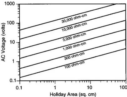
where ρ is soil resistivity and d the diameter of a circular defect having a surface area equal to that of the real defect. As we can notice, 𝑖_𝐴𝐶 is linearly proportional to the AV, while is indirectly proportional to the soil resistivity and to the defect diameter, i.e. 𝑖_𝐴𝐶 will be lower in a soil having a higher electrical resistivity and diameter. Figure 1.11 reports the value of the AV needed to have a 𝑖𝐴𝐶 of 100 A/m2, in function of the defect diameter and the soil

resistivity.

Figure 1.11 - AV needed to have a 𝑖𝐴𝐶 of 100 A/m2, in function of the defect diameter and the soil resistivity [20]

The ISO standard ISO 18086:2015 [16] specify that the local soil resistivity is controlled by the amount of soluble salts and by water content and is strongly influenced by the

electrochemical processes occurring on the metal surface in CP condition.

Really, the presence of a cathodic current causes the migration of cations towards the metal affected by CP and consequently the pH electrolyte increases in the vicinity of the metal. Depending on soil composition, the electrical resistance of the soil near the coating defect can either increase or decrease according to the pH increase.

The Annex D (informative) of ISO standard ISO 18086:2015 [16] reports the effect of earth-alkaline ions (as Ca2+ and Mg2+) and alkaline cations (as Na+, K+ or Li+) on the electrical resistivity and on the formation of salts and deposits at the interface between metal and environment. The former ones form hydroxides with relatively low solubility. The pH increase shifts the carbonate-bicarbonate equilibrium towards the precipitation of carbonates, with the formation of a calcareous deposit, leading to a coating defect resistance increase up to a factor of 100. In addition to this, the presence of earth-alkaline ions extends the passivity region expected from Pourbaix diagram of iron [5].

On the contrary, the latter ones form highly soluble hygroscopic hydroxides. Hence a low electrical resistance due to the high ions concentration is observed, decreasing the electric resistance at the coating defect up to a factor of 60. The current density on the metal at coating fault of a given geometry is, therefore, dependent on the electrical conductivity and the ratio of alkali and earth alkali ions. Moreover, the cathodic current density influences the amount of hydroxide produced and affects, therefore, the local conductivity.

The soil composition, in relation with the corrosion behaviour of metallic structures, is treated by other authors. For example, the ratio of alkali and earth alkali ions will be discussed in the following chapter, being the basis of the corrosion mechanism proposed by Voûte and Stalder [29]_{. Büchler et al.} [30] _{accentuated the importance of soil composition in}

the corrosion process: Ca2+ _{ions induce the formation of chalk layers on buried metal}

surfaces, leading to a modification in the electrical conductivity, and hence in the corrosion process, at the metallic-electrolyte interface.

In addition, the ISO standard ISO 18086:2015 [16] lists the soil resistivity parameters in terms of AC corrosion risk:

 below 25 Ω·m: very high risk;

 between 25 Ω·m and 100 Ω.m: high risk;  between 100 Ω and 300 Ω·m: medium risk;  above 300 Ω·m: low risk.

As mentioned before, increasing the soil resistivity reduces the effects of the AC density on the metallic structures.

1.3.6 Frequency effect

According to the studies [31,32,33], the frequency of the signal has an effect on AC corrosion: corrosion rate decreases by increasing frequency. Especially, AC at power frequencies of 50 or 60 Hz, that are commonly used in commercial apparatuses, can cause corrosion.

Fernandes [32] discussed a kinetic effect of frequency on corrosion: with the increase of frequency, the interval between successive anodic and cathodic half-cycles becomes shorter and the metallic ions formed in the anodic cycle would be available for the immediate re-deposition in the cathodic cycle. In addition, the author states that at high frequencies hydrogen atoms formed during the cathodic cycle haven’t enough time to coalesce and form hydrogen gas molecules. In this way, in the next anodic half-cycle, a layer of hydrogen atoms covers the metal surface and prevents the metal dissolution reaction.

In another study by Yunovich and Thompson [33], the current flow (corrosion current) through a steel specimen exposed to soil is calculated using an equivalent analog circuit (Randle’s model, Figure 1.12). The circuit consists of a double layer capacitance (C1), the solution resistance (𝑅_𝑆) and the “effective resistance” (𝑅_𝑒𝑓𝑓) that represents the combination of the charge-transfer and Warburg (diffusion-related) impedances.

Figure 1.13 - Electrical response of the circuit in Figure 1.12: the red line is the total AC, the green line is the AC passing through 𝑅𝑒𝑓𝑓[33]

The circuit also includes an AC power source (HVTL). The analysis allows to simulate the electric behaviour of the metal and to calculate the current passing through each component of an electric circuit varying the imposed AC frequency. AV is 24 V and AC density on the specimen is approximately 400 A/m2.

The current through 𝑅_𝑆 (related to corrosion process) and 𝑅_𝑒𝑓𝑓 (the total current in the circuit) is depicted in Figure 1.13, showing their dependence on the frequency of the AV applied by the AC source. The impedance of the capacitor (C1) and the current crossing 𝑅_𝑒𝑓𝑓 decreases with the frequency (going to zero when the frequency in infinite). Nevertheless, although most of the current at 60 Hz passes through the capacitor (C1) and thus does not affect corrosion reactions, there is an amount of AC (approximately 0.3% of the total current) that flows through 𝑅_𝑒𝑓𝑓 at 60 Hz frequency [33].

1.3.7 Corrosion Rate

The ISO standard ISO 18086:2015 [16] declares that evaluation of the AC corrosion likelihood can be determined by the corrosion rate on a probe, following the mechanisms described in Paragraph 1.4, above all the principle of the Electrical Resistance (ER) probe. In the literature many articles can be found about AC corrosion, and a large corrosion rate data variability can be collected. Nevertheless, only few essays contain information about the time-dependence of AC corrosion of carbon steel in CP conditions. In addition to that,

the available data are characterized by a significantly dispersion, so the correlation of the parameters associated to AC corrosion, such as AV and 𝑖_𝐴𝐶, and the corrosion rate is a difficult task.

One study was accomplished by Ragault [34] carrying out on-site experiments on a polyethylene coated steel gas transmission buried pipeline cathodically protected and parallel for 3 km with a 400 kV HVTL. The pipeline showed corrosion with corrosion depths equal to 0.1 up to 0.8 mm after one year of installation. In addition to that, also on-site experiments were carried out as close as possible to field conditions. 12 coupons were installed for 18 months close to the test posts where the worst cases of corrosion were found. Results showed that corrosion depth was comprised between 0.3 and 0.5 mm with AC density from 30 and 4000 A/m2 _{and on-potential between -2.0 and -2.5 V CSE. The author}

stated that there is no clear relation between AC density level and corrosion penetration depth, but high level of AC density may be an indication of high AC corrosion risk.

1.3.8 Morphology of AC corrosion

AC corrosion morphology is localized. Camitz et al. [35], in order to study AC corrosion, conducted a test consisting on cathodically protected steel coupons under different AC densities; the conditions of the two sets of tests were 10 V AC for almost two years and 30 V AC for 18 months. The goal of these experiments was to record the IR-free potential of the test coupons with an oscilloscope: the potential varied according to the AV signal and, during the positive half cycle, off-potential shifted in the anodic direction to values less negative than the limit value for CP, i.e. CP was periodically lost due to AC interference. In several cases, the potential shifted to values even less negative than free corrosion potential. Corrosion attacks could be classified into three groups:

 small point-shaped attacks evenly distributed across the surface (uneven surface);  large point-shaped attacks evenly distributed across the surface (rough surface);  few large, deep local attacks on an un-corroded surface (“pocked” surface).

The type and composition of these attacks depend on the structure affected by AC corrosion and also on its environment. Some example of studies based on the defect nature are listed below. Nielsen and Cohn [36] _{described a corrosion tubercle of “stone hard soil” comprising}

a mixture of corrosion products and soil often observed to grow on the coating defect surface in the presence of AC interference, which is depicted in Figure 1.14. It was demonstrated

that the specific resistivity of the tubercle is significantly lower than the specific resistivity of the surrounding soil. In addition, the effective area of the tubercle is considerably greater than the original coating defect. The combination of these parameters causes a decrease in the spreading resistance of the associated coating defect during the corrosion process, making the corrosion process autocatalytic. The studies conducted by Ragault [34] _and

Williams [37] are compliant on the fact that the main corrosion product on steel interfered by AC is magnetite, sometimes combined with soil. Wakelin et al. [20] reported that the aspect of the pit site could help to determine if AC corrosion is the primary cause of the failure.

Figure 1.14 - Schematic illustration of the tubercle of “stone hard soil” that grows at the coating defect in connection with AC corrosion [36]

Ellis [38] reported that the AC corrosion occur forming hemispheric attacks (in which the pH could be high) covered by hard corrosion products. Bolzoni et al. [39] proved again that AC corrosion has a localized nature.

1.4 AC CORROSION MONITORING

The ISO standard ISO 18086:2015 [16] reports that the driving force of the AC corrosion process is the alternating voltage (AV) occurring on the metallic structures. Additionally, the corrosion damage induced on the pipeline by AV depends also on AC current density, level of DC polarization, defect geometry, local soil composition and resistivity.

The standard states that there are three different approaches to prevent AC corrosion:  to limit the AC current flowing through a defect;