ALMA MATER STUDIORUM - UNIVERSITÀ DI BOLOGNA SCUOLA DI INGEGNERIA E ARCHITETTURA
CAMPUS DI CESENA
DIPARTIMENTO DI INGEGNERIA INDUSTRIALE
CORSO DI LAUREA IN INGEGNERIA BIOMEDICA
TITOLO DELL’ELABORATO
IN VITRO CHARACTERIZATION OF THE PRIMARY STABILITY OF ACETABULAR HIP IMPLANTS
Elaborato in
Comportamento Meccanico dei Materiali e Biomateriali (LT)
Relatore presentata da
Chiar.mo Prof. Luca Cristofolini Anisha Tresa Azhakathu
Co-Relatore
Ing. Federico Morosato
Sessione II
5 CONTENTS
ABSTRACT ... 7
RIASSUNTO ... 9
1. INTRODUCTION ... 11
1.1. TOTAL HIP ARTHROPLASTY ... 11
1.1.1 What is total hip arthroplasty? ... 11
1.1.2 Short history of THA... 12
1.1.3 THA in Italy... 13
1.1.4 Hip prosthesis: materials... 14
1.1.5 Cemented and cementless prosthesis ... 16
1.2 PRIMARY STABILITY OF THE ACETABULAR COMPONENT ... 17
1.2.1 Clinical evaluation of the primary stability ... 19
1.2.2 In vitro evaluation of the primary stability... 20
1.3 THE ROLE OF STRAIN IN THE CUP IMPLANT STABILITY... 25
1.3.1 DIC: Digital Image correlation ... 26
1.4 AIM OF THE THESIS... 28
2. MATERIALS AND METHODS ... 29
2.1SPECIMEN PREPARATION ... 29
2.2CUP IMPLANTATION AND SPECKLE PATTERN PREPARATION ... 30
2.3TESTING PROCEDURE... 31
2.3.1LOADING CONFIGURATION AND PROTOCOL ... 31
2.3.2 DIC motion measurements... 33
3. RESULTS AND DISCUSSION ... 35
3.1TRANSLATIONS AND ROTATIONS ... 35
3.2STRAINS ... 38
4. CONCLUSION ... 41
APPENDIX ... 43
A PROCEDURE FOR ANATOMICAL MEASUREMENTS ... 43
BIBLIOGRAPHY ... 55
FIGURES ... 57
7 ABSTRACT
Total hip arthroplasty (THA) is a surgical procedure consisting in the replacement of the hip joint with an artificial prosthesis. THA is widely performed worldwide, more than 600.000 THAs are performed in Europe every year. Hip replacement is indicated for the treatment of diseases causing pain and functional limitations such as osteoarthritis, dysplasia, Paget’s disease or trauma. More than 90% of the patients undergoing THA obtain pain relief and functional improvement. Nevertheless, there are cases of premature failure of the implant due to different causes. The most common cause of failure of the hip implants is aseptic loosening, in particular more than 50% of failures are associated to the aseptic loosening of the acetabular component. The primary stability of an implant is its capability to resist excessive motion at the bone-implant interface during the first post-operative period. The primary stability is a crucial aspect that influences the long term success of the hip surgery. In this thesis, a comparison between the primary stability of the acetabular component after two different type of surgical implantations has been done. Ten human cadaveric hemipelvis were used for this study. The specimens were cleaned, aligned and potted. Afterwards, a surgeon implanted uncemented cups in the specimens. The first time the depth of the cup was chosen in order to restore the native centre of rotation of the acetabulum. The specimens were tested simulating a simplified standing-up configuration. Packages of 50 cycles were applied. Each package was 10% higher than the previous one and the stopping criterion was a permanent migration greater than 0.5 mm or strain greater than 2000 . DIC (Digital Image Correlation) cameras were used to track the strain distribution on the bone surface during the test. The post processing of the DIC measurements allowed the evaluation of the micromotions at the bone-implant interface. After testing the specimens for the first time, the cup was extracted and the acetabulum was reamed until the base (lamina quadrilatera) before re-implanting the same cup. After the re-implantation, the testing procedure was repeated. The micromotions at the bone-implant
8
interface were measured, in particular permanent translation, permanent rotations, inducible translations and inducible rotations were analysed. The difference between none of these values was statistically significant. Maximum principal strains and minimum principal strains were evaluated on the bone surface. The difference between the maximum principal strains was not statistically significant, meanwhile the difference between minimum principal strains was statistically significant. The primary stability of an implant relies mainly on the micromotions at the bone-implant interface. Therefore, in conclusion, there is no statistically significant difference between the two implantation techniques as regards the primary stability. Thus, it should be preferred the use of the first implantation technique, because it allow to preserve more host bone and the amount of the host bone is an important clinical parameter considered by the surgeons in case of revision arthroplasty to choose the type of revision reconstruction.
9 RIASSUNTO
L’artroplastica d’anca è un’operazione chirurgica che consiste nella sostituzione dell’articolazione del bacino con una protesi artificiale. È una procedura ampiamente diffusa a livello mondiale e più di 600.000 artroplastiche d’anca vengono effettuate ogni anno in Europa. L’impianto di una protesi d’anca è indicato in casi di malattie che causano dolore e problemi motori, come osteoartrite, displasia o traumi. Più del 90% dei pazienti che si sottopongono all’intervento di artroplastica d’anca ottengono alleviamento del dolore e miglioramento della funzionalità articolare. Tuttavia, ci sono casi di fallimento dell’impianto dovuto a varie cause: la causa principale del fallimento è data dalla mobilizzazione asettica. In particolare, più del 50% dei casi di fallimento è dovuto alla mobilizzazione asettica della componente acetabolare. La stabilità primaria di un impianto può essere definita come la sua capacità di resistere ai micromovimenti che si verificano all’interfaccia osso-impianto nel primo periodo post-operatorio. La stabilità primaria è un aspetto fondamentale che caratterizza la vita a lungo periodo dell’impianto. In questa tesi è stato fatto un confronto della stabilità primaria della componente acetabolare dopo due diversi impianti eseguiti con tecniche diverse. Lo studio è stato svolto su dieci emi pelvi da donatori umani. Ciascun provino è stato accuratamente pulito e allineato. Gli impianti sono stati eseguiti da un chirurgo: durante il primo impianto l’obiettivo era quello di ripristinare il centro di rotazione dell’acetabolo nativo. Successivamente, i provini impiantati sono stati testati su una macchina di prova, simulando una condizione semplificata di standing-up. Sono stati applicati pacchetti di carico crescenti, partendo da un precarico pari al peso corporeo del soggetto. Il criterio d’arresto prevedeva una deformazione superiore a 2000 o una migrazione permanente superiore a 0.5 mm. L’utilizzo della Digital Image Correlation (DIC) ha permesso l’acquisizione di immagini cui elaborazione ha fornito informazioni sui micromovimenti all’interfaccia osso-protesi e sulla distribuzione delle deformazioni sulla superficie ossea. Dopo aver testato i provini per la prima volta, la protesi è stata estratta e ri-impiantata. Prima del secondo impianto, l’acetabolo è stato fresato fino a raggiugere la base (lamina quadrilatera). Dopo il secondo
10
impianto, è stata ripetuta la procedura di test con carichi crescenti e medesimo criterio d’arresto. Il confronto tra i micromovimenti all’interfaccia, in particolare delle traslazioni permanenti e inducibili e rotazioni permanenti e inducibili, non ha evidenziato differenze statisticamente significative tra le due tecniche di impianto. L’analisi delle deformazioni ha evidenziato differenze statisticamente significative tra le deformazioni principali minime, mentre la differenza tra le deformazioni principali massime non è risultata statisticamente significativa. Considerando che la stabilità primaria di un impianto dipende principalmente dai micromovimenti all’interfaccia, si può concludere che non ci sono differenze significanti tra le due tecniche di impianto. Tuttavia, può essere preferibile l’uso della prima tecnica di impianto considerata, in quanto permette di preservare una quantità maggiore di osso del paziente e la quantità di osso è un parametro clinico importante in caso di interventi di revisione.
11
1. INTRODUCTION
1.1. Total hip arthroplasty 1.1.1 What is total hip arthroplasty?
Total hip arthroplasty (THA) is an orthopaedic procedure consisting in the surgical replacement of the hip joint with an artificial prosthesis. This operation is indicted for the treatment of those diseases causing pain and functional limitation of the hip, when the medical therapy doesn’t work properly. During THA the head and the proximal neck of the femur is excised and the acetabular cartilage and the subchondral bone are removed. The metal stem of the hip prosthesis is inserted in an artificial canal created in the femur and a metallic shell is placed in the acetabulum.
The most common cause of THA is severe osteoarthritis of the hip, accounting for the 70% of cases1. This disease causes pain and limitation in daily activities. Other causes for which the procedure is indicated include dysplasia of the hip, Paget’s disease, trauma and osteonecrosis of the femoral head.
A great number of operations are performed every year worldwide and more than 90% of patients achieve complete pain relief and improvement in function1. For this reason, THA is considered one of the most successful orthopaedic interventions of the last decades: the operation of the century2.
Nevertheless, there are cases of complications that lead to the premature failure of the implant. In such cases, revision total hip arthroplasty is necessary. Causes of failure are multiple and can involve the femoral stem, the acetabular cup or both. Implant motion is the most frequent cause of failure. It is manifested by absorption of bone around the implant and it is detected radiographically before the patient has pain. Loosening may be mechanical or biological. Mechanical loosening results from excessive loading because of overuse, poor prosthetic design or improper insertion technique. Biological loosening results from bone resorption mediated by cells stimulated by the presence of wear debris from cement, polyethylene or metal.
12
The most common causes of dislocation include inadequate patient compliance with post-operative precautions and malposition of the acetabular component. Periprosthetic osteolysis is the result of an immune response taken up by macrophages and multinucleated giant cells. The presence of wear debris can cause the release of cytokines, resulting in inflammation which activates osteoclasts and finally leads to implant loosening.
1.1.2 Short history of THA
The first recorded attempts to replace hip joint occurred in Germany in 1891. Professor Themistocles Glück presented the use of ivory to replace femoral heads of patients whose hip joints had been destroyed by tuberculosis.
In 1925, the American surgeon Marius Smith-Petersen created the first “mold arthroplasty” out of glass. Even though the biocompatibility of the glass, it couldn’t resist the great forces going through the hip joint.
Philip Wiles developed first prosthetic arthroplasty in 1938 and the first to use a metal-on-metal prosthesis was the English surgeon George McKee, in 1953. He proposed a new one-piece CrCo socket as acetabulum. This method had good survival rate, but it caused the release of metal particles in patient’s body.
The English orthopaedic surgeon Sir John Charnley is considered the father of modern THA. In the early 1960’s he designed the low friction arthroplasty. It consisted of three parts: a metal femoral stem, a polyethylene acetabular component and acrylic cement. The design was very similar to the prosthesis still used in orthopaedic field and it became a gold standard for hip replacement. (Fig. 1)
13
Fig 1: Charnley’s low friction arthroplasty 1.1.3 THA in Italy
THA is a procedure widely performed in the world today. More than 600.000 THAs are performed in Europe every year3.
The Register of Orthopaedic Prosthetic Implants (RIPO) is a database that gathers information about the prosthetic implants performed in Emilia Romagna, including clinical conditions of the patients, surgical procedure and type of fixation. RIPO was initiated in 1990 and by December 31st, 2018, the Register collected data for about 125.000 hip prosthesis.
In 2016, data about 7659 primary THAs was reported, with an increment of 120 cases compared to the past years. The mean age of surgery is stable around 70 years for women and 66 for men. The register also reports an increasing use of uncemented prosthesis (62% in 2000 and 96% in 2016). The survival level of hip prosthesis registered in Emilia Romagna is very high: 89% of the prosthesis implanted are still in place after 17 years. The survival is lower for male and young patients.
14 1.1.4 Hip prosthesis: materials
During normal ambulation, the human hip has to withstand cyclic loadings comparable to forces three to five times the body weight. During more strenuous activity, such as running or climbing, the joint is exposed to much greater forces, as much as 12 times the body weight4.
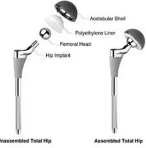
The hip prosthesis is designed to maximize the support of the implant during the daily activities and to closely approximate the function of the natural hip joint. The hip prosthesis is composed by a metallic stem which is inserted in the femur, a metallic shell placed in the acetabulum, a head and a liner. (Fig. 2)
Fig 2: the components of a hip prosthesis
Nowadays, the stem and the cup are realized in titanium alloys. High mechanical strength, excellent corrosion resistance and biocompatibility makes Ti6Al4V a good choice for the cementless prosthesis.
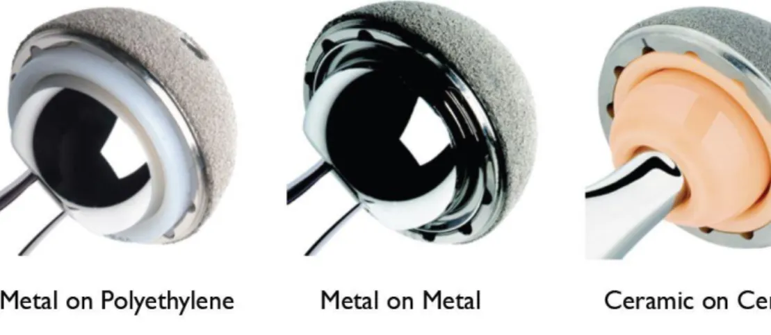
Several materials are currently adopted to create the femoral head and the acetabular liner (Fig. 3). The combination of the materials used to realize the different components of the hip prosthesis is intended to reduce the friction and wear phenomena.
• Metal on UHMWPE provides a safe and cost-effective technique, and for many represents the gold standard in THA4. The main concern regarding this combination of materials is the release of polyethylene debris causing a
15
biological response and leading to osteolysis and implant failure due to aseptic loosening. Polyethylene is commonly sterilized using gamma rays, but this procedure causes the release of free radicals which oxidizes in the presence of air. The oxidation makes PE less resistant and more brittle, increasing the wear phenomena.
• The metal on metal prosthesis have lower incidence of dislocation, because the metal femoral heads are less brittle than other materials and they can have larger diameter, increasing joint stability. Stainless steel was the first alloy introduced in orthopaedic practise: iron-carbon based alloys that may contain also Cr, Ni, Mo, Mn and C. The austenitic alloys (316 series) are commonly used to produce prosthesis. Nowadays, CrCo alloys are also used because of their strength and resistance to corrosion and wear. The disadvantage of metal-on-metal bearings is the generation of metallic ions (metallosis), which can be cancerogenic and it is also associated with prosthetic loosening. In order to achieve osteointegration and to prevent loosening, porous metallic cups are used.
• The ceramic-on-ceramic combinations have a very low level of friction and excellent wear resistance. The benefits of ceramic on ceramic prosthesis are also the high level of hardness, scratch resistance and inert nature of the ceramic materials. Wear observed in ceramic on ceramic bearing is a few microns for a 15-years period, which is about 2000 times less than a metal on polyethylene combination and 100 times less than a metal on metal prosthesis5. However, this type of prosthesis isn’t used frequently, because they are expensive and they also have a high risk of fracture compared to the other materials.
16
Fig 3: different bearing surfaces used in THA 1.1.5 Cemented and cementless prosthesis
Today, in clinical practise, mainly two types of hip implant fixation techniques are used: cemented and cementless. In the cemented prothesis, a layer of acrylic resin, generally polymethylmethacrylate cement, is put between the bone and the prosthesis to ensure stability. The cement fills the space between the bone and the prosthesis, enlarging the contact surface, minimizing the prosthesis micromovements and ensuring the load transmission from the prosthesis to the bone. Addition of barium sulphate (BaSO4) to the cement ensures radiopacity. In some cases, antibiotics or vitamin-E are added to the cement to reduce infections and inflammatory processes, with only modest reduction of the mechanical stregth6.
In the cementless prostheses the press fitting technique is used, a biological fixation is obtained by the bony ingrowth into a porous coating on the implant. The latest porous metal components have an average volume porosity between 60% and 75% and a surface porosity of 80%, an average pore size between 200 and 616 µm and a coefficient of friction between 0.65 and 1.2. The bone ingrowth into porous implants using tantalum or titanium porous coating occurs after only 2-3 weeks7. The cementless THA was developed in response to the fact that cement debris released at the bone-implant interface caused loosening and failure of the cemented implants. Preliminary data suggest that cementless technique has a relatively low revision rate and excellent prosthetic durability for as long as 15 years1. In young patients, where a future revision is more likely and the implant is
17
highly stressed, the non-cemented technique is preferred. In addition, in the young the bone is more active and the osteointegration occurs easily.
On the other hand, the cementless prostheses require a healthy bone, so they cannot be used on weak, osteoporotic bone. Cemented replacement is mainly used for old, less active people or on patients with weak bones. Better short-term clinical outcome, particularly regarding the pain improvement, can be obtained with cemented fixation8. People with uncemented implant should limit their activities for up to three months and the cementless surgery can cause thigh pain for several months after surgery9.
In summary, both cemented and cementless prostheses are available in clinical practise. The choice between the two depends on many factors, such as the patient’s physical demand and the quality of the bone.
1.2 Primary stability of the acetabular component
Even if the previous considerations are applicable both to the femoral stem and acetabular component, nowadays, more than 50% of the hip implants failures is associated with the loosening of the acetabular component7. For this reason, the focus of the next chapters of the thesis will be on the acetabulum.
In the cementless procedures, the prosthesis is press fitted into the bone cavities. The primary stability of the implant is a crucial aspect that determines the long time success of the hip surgery. It can be defined as the capability of the cup to resist to excessive motion at the bone interface in the first post-operative period. The primary stability depends on several factors including the pore size and rough surface of acetabular component, the quality of underlying bone and the snug fit between the implant and the host bone. Also the cup geometry and the surgical technique used are important factors. Stability depends on the area of interface contact between the cup and the bone. If the dimension of the cavity is too small or too big, the cup will not fit well and the primary stability is compromised. Cups with a true hemispherical profile are more stable than the other cups, because they maximize the contact area with the bone. The use of acetabular cavities 1-2mm smaller than the cup appears to gain more stability10.
18
For successful osteointegration to occur (secondary stability), only minimal relative motion between the implant and the host bone is allowable.
In fact, micromotion at the bone-implant interface may induce the development of fibrous tissue around the implant, which could be responsible of the aseptic loosening. Histological analysis of the fibrous tissue has shown the presence of cells like macrophages, fibroblasts and foreign body giant cells, so the immune system is involved in the formation of such a membrane at the interface11.
In order to avoid formation of fibrous tissue at the interface and to allow osteointegration, the cup motions must be lower than 100-200 μm12.
Cup motion can be divided into two categories: permanent migration and inducible micromotion. Permanent migration is the non-reversable migration that is accumulated during daily activities. Excessive permanent migration (in order of 1mm) observed in the first post-operative follow up is a predictor of late loosening of the implant13. Inducible micromotion is the reversable motion that occurs between loading and unloading.
To reduce this incidence of aseptic loosening numerous modifications have been made over the last years to promote the fixation of the implant to the host bone. The use of adjunctive screws is helpful particularly in cases of bone defects. Other modifications have focused on prosthesis materials and adaptations of the cup design, like the addition of fins and pegs. (Fig 4)
19
1.2.1 Clinical evaluation of the primary stability
Clinically, the primary stability is evaluated using radiographic images. The simplest way to assess migration of the acetabular cup is comparing radiographs of different follow-ups. This procedure is affected by errors due to variation in the positioning and rotation of the patient, differences in focusing and film centring. Various anatomical features have been considered to minimize the errors committed by clinicians while assessing the cup migration, but the reliability of this method is still uncertain. There are also analytical errors due to intra-observer and interobserver variability15.
Furthermore, the radiographic images are obtained with the patient still in a position, so it is not possible to evaluate what happens during a specific activity. Another issue related to the radiographic assessment method is that it may take several years before the final stages of aseptic loosening are visible. Yet, plain radiographic methods are used because of their worldwide diffusion, availability and ease of use. Moreover, they are cheap and they don’t require sophisticated equipment.
RSA (Roentgen stereophotogrammetric analysis) is considered the gold standard for clinical assessment of cup migration15. It consists in the implantation of tantalum marker beads onto the bone around and in the prosthesis and the prosthesis migration is measured using 2 radiographs obtained from two different angles. This is a precise and accurate procedure that allows an early detection of loosening13. RSA studies are able to detect unsafe acetabular cups 2 years postoperatively. RSA evaluates the short term loosening, but it cannot detect later events that affects the prosthesis failure rate, such as loosening caused by wear-induced osteolysis or fracture in the cement, in case of cemented prosthesis. Furthermore, RSA requires sophisticated equipment, it is time consuming and it can be used only in patients with marker beads.
Another method used in clinical practise is EBRA. This technique differs from the other methods because it uses an algorithm that excludes from a patient measurement series of radiographs those images that have more than a defined level of positioning or rotational error. The data from EBRA studies suggest that
20
the use software to exclude non comparable radiographs increase precision. The main weakness of EBRA is that, because of the quality control algorithm, some data is lost if the radiographic projections are not similar.15
1.2.2 In vitro evaluation of the primary stability
Although the measurement techniques previously explained are the only methods clinically available to assess the stability of the cup, in many cases it may be interesting to evaluate the primary stability of the cup using higher accuracy and precision, for example before performing clinical trials.
Clinical trials are research investigations used to estimate in vivo the reliability of new devices, implant techniques or fixation techniques. In this case, in vitro studies are much more reliable than the tools adopted in clinical practise.
With in vitro studies it is possible to observe micro and macro migrations of the cup, but, most importantly, it allows the monitoring of the elastic movements. As in real life, many factors are involved in the stabilization of the hip joint (muscles, bone quality, force direction, posture…). Inevitably, in vitro tests rely on replication on simplified models. These simplifications may be related to the bone model, loading conditions or measurement of the clinical parameters. A. Bone models
Simple models use foam blocks with a hemispherical cavity as an acetabular model. These blocks are easily available, cheap and have constant mechanical characteristics.
Use of polyurethane specimens permits to simulate different type of bone by choosing the density of polyurethane used. The bone density range is comprised between 0.17 and 0.50 g/cm3, and the compressive strength between 2 and 50 MPa. Correctly chosen polyurethane foams simulate either normal bone, if the its density is near the top of the bone density range, or weak (for example, osteoporotic) bone, if the density of the specimen is near the bottom of the bone density range16. Using polyurethane blocks also avoids the issue of interspecimen variability, but it does not consider the anatomical features of the acetabulum. Studies demonstrated that using a spherical cavity to model the acetabulum may
21
overestimate the stability of press fit acetabular cups16. Another limitation of the polyurethane specimens is that the stiffness of the cortical bone is not considered and, as the primary stability depends on the capability of the cup surface to grip the bone cortex, these models are limited to the simplified studies only.
Animal models are used alternatively to the synthetic models, since the animal bone has more similar mechanical characteristics (i.e. they have cortical bone and trabecular bone) to the human bone than synthetic models. However, animal bone presents a different yield and fracture behaviour and the anatomy is slightly different from the human model. Moreover, unlike the polyurethane models, the animal bone has to be conserved and treated carefully.
Simple models allow the comparison between different prothesis or between different implant techniques, since there is no interspecimen variability, but they are not ideal to study the mechanical behaviour of the bone.
As regards anatomical models, either composite or cadaveric human specimens can be used.
Composite specimens overestimate the cortical bone stiffness and underestimate the viscoelastic behaviour, but they represent a good compromise between the previously described synthetic models and the cadaveric specimens, because they have low variability and low costs.
Cadaveric specimens have more variable characteristics, but those are the most reliable specimens which allow a reasonable representation of the real scenario. In fact, they not only have the same elastic modulus of human bone, but they also present yield behaviour similar to the living bone. The main issues related to the cadaveric specimens are the costs and availability. Moreover, the conservation process and the handling of the human specimens can represent an issue for many research labs. Normally, the soft tissues are removed before testing and, in order to conserve the mechanical properties of the bone, cadaveric specimens should be kept wet during the test.
22 B. Loading conditions
Many forces are involved in the movement of the hip during a motor task: muscle forces, body weight, ligament tensions and other external forces. In vitro studies usually consider a resultant of all those forces17,18.
The hip undergoes forces that are several times the body weight during a motor task. For example, during walking, the forces on the hip are about 2-3 times the body weight. The primary stability describes the capacity of the implant to resist to similar loads. In simple models, the cup is forced to migrate in a specific direction, meanwhile in other models, more complex loading conditions are considered:
B1) Torsion test: loads are applied through a rod connected to the acetabular cup. The applied load is generally a combination of a torsional and a compressional force. The load and the displacement are measured by the testing machine. Torsion tests allow to measure the displacement on the plane of the acetabular cup. (Fig 5)
Fig 5: example of mechanical setup for torsional testing of cup stability10.
B2) Lever out test: a controlled eccentric load is applied and the force necessary to distract the cup is registered. This type of test allows to measure the displacement out of the acetabular plane. (Fig 6)
23
Fig 6: example of lever out test10.
B3) Pull out and push out tests: during pull out tests, a tractional load is transferred to the cup through a rod firmly fixed to the cup. The force necessary to distract the cup is registered. In push out test, a compressive force is applied instead of the tractional load. (Fig 7)
24
B4) Physiological loading: different directions of the load, representative of a specific motor task, are considered in physiological models. The specimen is aligned properly to reproduce particular loading conditions. (Fig 8)
Fig 8: example of physiological model simulating a leg stance19
C. Measurement of clinical parameters
During the application of different loading conditions, in order to evaluate the primary stability of the cup, the relative motion between the implant and the bone has to be measured. The relative motion is the combination of rotations and translations in the 3D space.
Linear variable differential transformers (LVTDs) can be placed on the specimen surface to evaluate the relative motion between bone and the implant20. To measure the translation in the three directions of the space, at least three orthogonal LVDTs have to be used. The use of linear transductors is accurate and precise, but they provide pointwise measurements and they are not able to measure the strains of the bone surface. Another issue related to the use of LVTDs is that, in order to obtain reliable measurements, a rigid fixation of the transductors to the bone has to be ensured. Any accidental change in the alignment of the sensors can affect the quality of the final outcomes.
25
Optical systems can also be used: high resolution optical position markers are placed on the cup and the liner and the 3D migrations are measured7. The main disadvantage of this method is that the markers must be visible during the entire test.
The use of Digital Image Correlation can overcome the problems previously presented. It allows the measurement of the displacement and the strain on the whole bone surface referred to a fixed reference frame.
1.3 The role of strain in the cup implant stability
Generally, when assessing primary stability, only the micromotions are measured. But it is also important to evaluate the strain distribution in the bone. For example, the strain can be an indicator of the stress shielding, a mechanical phenomenon that causes bone loss and lead to the implant failure. Stress shielding is caused by the alteration of the stress distribution in the bone following the implantation of the prosthesis. Different factors influence the occurrence of this event: relative bending stiffness, the design of the implant, the size, shape and density of the host bone and the material composition.
To avoid stress shielding and bone loss it is important to allow load transfer from the implant to the bone, because continuous unloading of the bone leads to the bone absorption. This phenomenon is explained by the Wolff’s law: the bone adapts itself in response to cyclic loading21.
After the implantation of the prosthesis the physiological loads are distributed between the bone and the implant. Since the Young modulus of elasticity is different for the bone and the implant material, also the stress distribution in the host bone changes. (Fig 9)
26
Fig 9: Young’s modulus and density of common biomaterials.
The bone optimizes its shape and mass in order to have a uniform stress distribution and to minimize the metabolic energy consumption. Therefore, if the cyclic loads on the bone are lower than the physiological loads, the bone absorption occurs and this event leads to the implant failure.
To lower the excessive stiffness of femoral stems, it is possible to modify the design or to use materials with a lower elastic modulus, such as titanium. Also the addition of bioceramics (tricalcium phosphate) to proximal hydroxyapatite-coated stems has shown good results regarding the conservation of bone mineral density.
1.3.1 DIC: Digital Image correlation
While it is not possible to measure the strains clinically, in vitro studies allows the evaluation of the strain distribution on the bone surface. Some studies in literature rely on the use of strain gauges22. Even though the measurements are precise and accurate, strain gauges provide a pointwise measurement, and not the strain distribution on the entire bone surface. Moreover, strain gauges are sticked to the bone surface with glue, and the layer of glue between the bone and the strain gauge may affect the outcomes.
The displacement and strain distribution on the bone surface are measurable, overcoming the previous problems, using Digital Image Correlation (DIC). This
27
technique allows to assess the strain and displacement distribution on the whole visible surface of the test object. It is a contact-less method that obtains information on strain and displacement comparing series of images of unloaded and loaded bone. The bone surface must have a high contrast random pattern, so the DIC software can recognize univocally portions of bone and track them through the different images. Displacement is calculated comparing different frames and the strain is obtained by differentiation. A single camera is used in 2D implementation and a set of two calibrated cameras ensures the 3D implementation.
The acquired images are divided into smaller areas, called facets. Each facet is computed separately by the software to obtain the displacement field on the bone surface. Therefore, a higher number of facets means an increased computation accuracy. Also the size of the single facet affects the results: larger facets grant better identification and correlation in subsequent images and the measurement of displacement and strain is more accurate and less affected by noise. But the use of large facets also means loss of information and high computational cost, which is proportional to the square of the facet size. Adjacent facets must be overlapped by a certain number of pixels to prevent loss of information.
The surface of the bone analysed by DIC should have a random high contrast pattern, for example black speckles on white background. Normally an airbrush gun is used to paint the specimen surface. The pattern must be casual, so each facet is univocally recognizable and the fraction of the area covered by the speckles should be same as the portion where there is only the background. (Fig 10) An optimal speckle pattern should have the minimum speckle dimension between 3 and 5 pixels23.
The paint used to create the speckle pattern should not modify the bone characteristics and the layer of the paint should move and deform with the underlaying bone.
28
Fig 10: speckle pattern preparation
1.4 Aim of the thesis
The aim of the thesis was the in vitro evaluation of the primary stability of acetabular implants, focusing on the effect of different implantation techniques. In particular, I measured:
• Relative movement between the implant and the surrounding bone, in terms of translations and rotations.
• Full field strain distribution around the acetabulum. All the measurements were conducted using the DIC software.
29 2. MATERIALS AND METHODS
Ten human cadaveric hemipelvis were used in this study (Tab 1). First of all, the soft tissues were removed from the bone surface. Afterwards, the specimens were aligned and potted to ensure consistent testing conditions. Anatomical measurements, necessary for the future steps, were performed on each hemipelvis. We tested the specimens in two different implantation configurations: shallow and deep implants. After the implantation, a speckle pattern was painted on the bone and the cup. A DIC system was used to track the position of the cup and the bone during the test and to measure the strain distribution on the bone surface.
Tab. 1: : List of hemipelvises used in this study, including the donors’ details and the size
of the implanted cups
2.1 Specimen preparation
We prepared ten human cadaveric specimens for the tests.
The specimens were accurately cleaned and all the soft tissues were removed, without damaging the underlaying bone, especially in the periacetabular area. (Fig 11) Donor Cause of death Sex Age (years) Height (cm) Body weight (kg) BMI (kg/m^2) Side Cup size (mm) #1 Sepsis Female 83 164 62.5 23 L 56 R 56 #2 Respiratory paralysis Male 70 175 79 26 L 52 R 54 #3 - Male 74 176 78 25 L 48 R 48 #4 Coronary thrombosis Male 71 187 92 26 L 60 R 62 #5 Cardiac arrhythmia Male 61 181 96 29 L 56 R 54 Median SD
30
Fig 11: human cadaveric hemipelvis
In order to define a reproducible testing condition, the specimens have to be potted before mounting it on the testing machine. For this reason, each specimen was aligned in a reliable reference frame and potted in an aluminium pot with bone cement. The alignment was performed following a procedure defined previously.24 Anatomical measurements were done on each specimen. In particular, the following parameters were measured: distance between anterior column and acetabular axis, distance between posterior column and acetabular axis, the height of the centre of rotation (CoR) of the acetabulum, the distance between the centre of the aluminium pot and the CoR and the medial wall thickness of the acetabulum. These measurements were useful for the following steps of the study.
Concerning this topic, I produced a document for the laboratory (see Appendix).
2.2 Cup implantation and speckle pattern preparation
A surgeon implanted uncemented cups in each specimen. The cup size was chosen based on the previous measurements and the surgeon’s experience. During the first implantation (COR- implantation), the depth of the cup was chosen as to restore the native CoR. After each implantation, position of the centre of the cup was measured and compared to the native CoR. A difference greater than +2mm required a re-implantation.
31
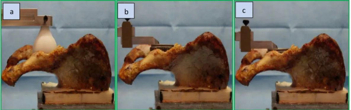
After testing all the specimens in the first configuration, the cup was extracted from the acetabulum. The surgeon reamed the acetabulum until the medial cortical bone under the base of the acetabulum (lamina quadrilatera) was reached. Then, the cup prosthesis was re-implanted (LAMINA-implantation) and the testing procedure was repeated. (Fig 12)
Fig 12: specimens during anatomical measurements (a), after CoR implantation (b) and after LAMINA implantation (c).
Before performing each biomechanical testing, in order to allow to the DIC software to correctly track and correlate the bone displacements and strains, a speckle pattern was painted on the implanted specimens’ surface. A high contrast black on white pattern was made using airbrush-airguns. First, the bone surface was covered with water-based white paint diluted at 50% with water. Afterwards, black speckles were painted using water based black paint, diluted at 25%. The pressure and other parameters of the airbrush-airgun like the airflow and the spraying distance were optimized to obtain the ideal dot size.
2.3 Testing procedure
2.3.1 Loading configuration and protocol
During the tests, we examined how the standing up form seated motor task affects the primary stability of the acetabular cup and the strain distribution on the bone surface, comparing two different types of implantation techniques.
Generally, in vitro studies simulate the walking condition, since it is the most common activity done by a patient undergoing THA in the first post-operative period. But, also other activities are carried out by patients after hip arthroplasty, such as standing up from seated, cycling and climbing upstairs. In our studies the
32
standing up condition was simulated, because it induces a large peak force in a completely different direction compared to the walking condition25. The potted specimen was mounted on an axial servo-hydraulic machine. Custom wedges were used to allow the transmission of the force in the desired direction from the actuator of the testing machine to the specimen. Simplified loading conditions were considered to simulate the standing-up. A single loading direction was defined to reproduce the peak force measured in vivo18. The force pointed medially and toward the lower part of the posterior column. Therefore, a single direction force was applied in increasing load packages, in particular, each package was 10% higher than the previous one:
Δ i+1 = 1.1* Δi
Each package was composed by 50 cycles (Fig 13). A precompression of 0.5 body weight was applied. The amplitude of the first loading package was 0.5 body weight.
Fig 13: loading protocol composed by packages of 50 cycles. Each package was 10% higher than the previous one. On the right, a specimen properly aligned in the testing
machine. The red arrow represents the direction of the applied force. Dic cameras
33
The test was continued until a permanent migration greater than 0.5 mm or strain greater than 2000µε was measured. The permanent migration was measured by the testing machine, while the strains were monitored by the DIC software.
2.3.2 DIC motion measurements
Two cameras were used in order to obtain 3D measurements.
The distance of the cameras from the specimen and the parameters of the cameras were chosen to frame the region of interest in an optimal way.
The region of interest included posterior column of the acetabulum and part of the cup liner: this allowed the monitoring of the relative movements between the bone and the cup and the strain distribution in the most critical regions of the bone. LED lights were placed near to the specimen to ensure a homogeneous view of the region of interest, avoiding formation of shadows or reflections.
Before testing each specimen, calibration was done using a dedicated calibration target. This procedure is used to define a reference frame for the DIC measurements.
The correlation parameters adopted derived from a previous optimization study26. In order to evaluate the permanent migrations and inducible micromotion during each loading cycle, the DIC measurements were post processed by a dedicated script in Matlab27. For each cycle of applied loads, the absolute translations and rotations were calculated in correspondence of each load-peak and load-valley. This procedure was done separately for the bone and the insert. The relative translations and rotations were calculated comparing the absolute roto-translations. Permanent migration and inducible micromotions were computed. The strain distribution was extracted directly on the DIC software.
35
3. RESULTS AND DISCUSSION
3.1 Translations and rotations
The correlation software was able to track the motions of the bone and of the cup throughout COR-implantation testing and LAMINA-implantation testing.
The relative bone permanent and inducible translations and the relative cup-bone permanent and inducible migrations were tracked (Fig 14).
Fig 14: example of trend for 3D permanent and inducible translations and permanent and inducible rotations tracked by the correlation software (AP= antero-posterior,
ML=medio-lateral, CC=cranio-caudal).
The single components of permanent translations were larger in COR-implantation than in LAMINA-implantation, but the difference was not statistically significant for any component of translation. The inducible translations were generally larger in COR-implantation, but the difference was not statistically significant for any component of translation. The Wilcoxon signed-rank test was used (Tab. 2,3).
T ra n sl a ti o n s (m m ) T ra n sl a ti o n s ( m m ) Ro ta ti o n s (° ) Ro ta ti o n s (° )
36
Tab. 2: The median values and the range (out of 10 specimens) of the 3D permanent
translations measured when the last load peak was applied are reported. The Wilcoxon signed-rank test was used for the statistical analysis.
Implantation Permanent translations (mm)
AP CC ML COR-implantation -0.054 (-0.167 ÷ 0.278) 0.049 (-0.027 ÷ 0.180) 0.079 (0.023 ÷ 0.217) LAMINA-implantation -0.029 (-0.149 ÷ 0.056) 0.026 (-0.101 ÷ 0.187) 0.023 (-0.005 ÷ 0.128) P-value 0.69 0.47 0.22
Tab. 3: The median values and the range (out of 10 specimens) of the 3D inducible
translations measured when the last load peak was applied are reported. The Wilcoxon signed-rank test was used for the statistical analysis.
Implantation Inducible translations (mm)
AP CC ML COR-implantation -0.011 (-0.094 ÷ 0.048) 0.019 (-0.048 ÷ 0.104) 0.043 (-0.001 ÷ 0.064) LAMINA-implantation -0.017 (-0.038 ÷ 0.008) 0.008 (-0.057 ÷ 0.085) 0.036 (0.005 ÷ 0.071) P-value 0.81 0.69 0.69
37
The permanent and inducible rotations have shown a variable trend. The difference was not statistically significant for any component of permanent rotation. As regards the inducible rotations, the difference was statistically significant for the rotations around the antero-posterior and medio-lateral axes (Tab. 4,5).
Tab. 4: The median values and the range (out of 10 specimens) of the 3D permanent
rotations measured when the last load peak was applied are reported. The Wilcoxon signed-rank test was used for the statistical analysis.
Implantation Permanent rotations (°)
AP CC ML COR-implantation -0.01 (-0.08 ÷ 0.0.27) 0.02 (-0.58 ÷ 0.52) -0.04 (-0.28 ÷ 0.59) LAMINA-implantation -0.08 (-0.19 ÷ 0.08) -0.01 (-0.15 ÷ 0.19) -0.09 (-0.30 ÷ 0.16) P-value 0.16 0.81 0.81
Tab. 5: The median values and the range (out of 10 specimens) of the 3D inducible
rotations measured when the last load peak was applied are reported. The Wilcoxon signed-rank test was used for the statistical analysis.
Implantation Inducible rotations (°)
AP CC ML COR-implantation -0.01 (-0.07 ÷ 0.07) -0.02 (-0.20 ÷ 0.07) -0.01 (-0.06 ÷ 0.15) LAMINA-implantation -0.03 (-0.13 ÷ 0.02) 0.003 (-0.05 ÷ 0.04) -0.03 (-0.10 ÷ 0.02)
38
P-value 0.03 0.69 0.02
Even if implant motions were generally larger in COR-implantation, results showed no statistical differences between the two implantation techniques in terms of primary acetabular stability.
3.2 Strains
Elaboration of the images obtained during the biomechanical tests by the DIC software allowed to measure the strain distribution on the bone surface. When the maximum load was applied in the last package, largest maximum principal strains () were localized in the superior part of the acetabulum. Conversely, the largest minimum principal strains () were localized in the superior-posterior region (Fig 15).
39
Figure 15: example of the strain distribution on the bone surface tracked by the DIC software. The strains were measured when the last load peak was applied to the
specimen.
The mean strain values are slightly higher than the physiological threshold (2000 ) in both COR and LAMINA implantation, but in the LAMINA-implantation some of the observed strain values are much higher than 2000 . The difference between the peak values of measured by the DIC software, was not statistically significant. The difference between the peak values of is statistically significant. (Tab 6).
40
Tab. 6: The median values and the range (out of 10 specimens) of the principal strains
measured when the last load peak was applied are reported. . The Wilcoxon signed-rank test was used for the statistical analysis.
Implantation Principal strains ()
COR-implantation 2107 (2042 ÷ 2262) -2117 (-2465 ÷ -1657) LAMINA-implantation 2233 (2110 ÷ 5205) -2543 (-3372 ÷ -2101) P-value 0.08 0.02
The primary stability of an implant is mainly associated with the micromotion at the bone-implant interface. Even if the difference between the minimum principal strains are statistically relevant, the other parameters, such as permanent and inducible translations and rotations, don’t show any differences between the COR-implantation and the LAMINA-COR-implantation. Therefore, there is globally no difference between the two implantation techniques.
41
4. CONCLUSION
The aim of the thesis was to evaluate the primary stability of acetabular implants, comparing the effect of two different implantation techniques. Ten human cadaveric specimens were prepared, aligned and a speckle pattern was painted on the surface of each specimen. Biomechanical tests were performed on the specimens after two different type of implantations: COR-implantation and LAMINA-implantation. During the first implantation the purpose was to restore the native centre of rotation of the acetabulum, while during the second implantation the surgeon reamed the acetabulum until the lamina quadrilatera. During the biomechanical tests, a simplified Standing-up condition was simulated. Increasing loading packages were applied to the specimens. The DIC software tracked the strain distribution on the bone surface and the permanent migrations and inducible micromotions were evaluated using a Matlab script.
Both COR-implantation and LAMINA-implantation are commonly used by surgeons in the clinical practise, but there is no evidence of differences between the two techniques.
The comparison between the two implantation techniques showed that the motions are generally larger in the COR-implantation and the strain distribution are higher in the LAMINA-implantation, but there is no statistically significant difference between the two implants as regards the primary stability of the acetabular component. For this reason, as COR-implantation allowed to preserve more host bone during the preparation of the hemipelvis (i.e. the reaming was shallower than LAMINA-implantation), COR-implantation could be preferred in clinical practice. In fact, in case of revision arthroplasty, the amount of host bone is a clinical parameter considered by surgeons for choosing which revision reconstruction (defect restoration, revision device, augmentation, screws...) to adopt.
43 APPENDIX
A procedure for anatomical measurements
This appendix describes a procedure for the measurement of specific anatomical features, required for future studies on human hemipelvis related to acetabular defects. In particular, such defects are implemented using a standard procedure based on:
• Native acetabular radius (NR): the size of acetabulum before implant insertion. (Fig 16)
• Minimum medial wall thickness (MT): the amount of the bone in the acetabular floor.
• Anterior column width (AW): distance between the acetabular centre of rotation and the outer rim of the anterior column. (Fig 16)
• Posterior column width (PW): distance between the acetabular centre of rotation and the outer rim of the posterior column. (Fig 16)
The definition of all the previous features must be intended with the specimen aligned with the acetabular plane horizontal.
44
Fig 16:top view of a virtual hemipelvis aligned with the acetabular plane horizontal. The anterior column width (AW) and the posterior column width (PW) are visualized. AW as the distance between the CoR and the outer rim of the anterior column and PW
as the distance between the CoR and the outer rim of the posterior column
A1. MATERIALS
- Reference table (Fig 1a)
- Aluminium pot with screws (Fig 1b) - Big L-square (Fig 1c)
- Small L-squares (Fig 1d) - Custom handle (Fig 1r) - Spherical plug (Fig 1f) - Caliper (Fig 1g)
- Aluminium block (Fig 1h) - Clamping key (Fig 1i)
- Long sharp Kirshner wire (Φ=2mm) (Fig 1j) - Short not sharp Kirshner wire (Φ=2mm) (Fig 1k)
45 - Ruler (Fig 1l)
- Vertical ruler (Fig 11)
Fig 1: tools used for the measurements. A2. Preliminary preparations
All the procedures must be performed on a reference table. (Fig 1a)
• Take the specimen and put it correctly inside the aluminum pot. Insert the 6 screws in the holes in the lateral walls of the pot to secure the specimen. (Fig 1b)
• Pick the spherical plug suitable for the specimen (check the specimen database). (Fig 1f)
• Measure the total length of the spherical plug (L) using the caliper. (Fig 2) TIP: remove the metal ring of the neck of the plug, if necessary.
46
Fig 2: measurement of l • Calculate l as l=L-radius of the sphere. (Fig 2)
• Insert the custom handle on the big L-square with the clamping screws not tighten, so you can move it along the L-square.
• Place the spherical plug in the terminal hole of the custom handle. (Fig 3)
47
• Place the aluminium pot with the specimen on the reference table and put the big L-square with the custom handle on the side of the posterior column. • Adjust the height of the custom handler so that the plug can be inserted inside
the acetabulum. Use the aluminium block to ensure that the custom handle is in square with the L-square. (Fig 4)
Fig 4: use of aluminium block
• Use the clamping key to tight the screws of the custom handle. • Take the long sharp Kirshner wire (Φ=2mm) and insert it in the drill • Insert the Kirshner wire in the through hole of the spherical plug. • Make a through hole in the bone with the drill. (Fig 5)
48 A3. MEASUREMENTS
• Align the aluminium pot and the big L-square with the edges of the reference table with the help of the small L-squares. (Fig 6)
TIP: be sure that the bases of the small L-squares used for the alignment are perfectly in touch with the edges of the reference table.
Fig 6: alignment of the aluminum pot with the edges of the reference table
• Insert the Kirshner wire in the through hole of the spherical plug. It will be used as reference point of center of rotation (CoR) of the acetabulum. (Fig 7)
Fig 7: Kirshner wire used as reference point for the CoR
A3.1 Measurement of the distance between anterior column and CoR
• Take a L-square and place it close to the anterior column. Put it in touch with the bone and visually align it with the Kirshner wire.
49
TIP: in case you were not able to put the L-square in touch with the bone, align it with the lateral edge of the aluminium pot instead.
• Take another L-square and align it with the edges of the reference table. TIP: take the ruler and put it in touch with the step of the custom handle to facilitate the alignment. Keep the ruler in touch with both Kirshner wire and L-square.
• Measure the distance between the L-square and step (a1) and the distance between the Kirshner wire and step (a2) and subtract them. (A=a1-a2)
• In case you were not able to put the L-square in touch with the bone, measure the distance between the L-square and the most prominent part of the anterior column (a3) and calculate A as A=a1-a2-a3. (Fig 8)
TIP: be sure to not lose the alignment of all the objects on the reference table. TIP: be sure that the ruler is always parallel with the reference table and in touch with the L-square.
Fig 8: Measurement of distance between anterior column and CoR
A3.2 Measurement of the distance between the posterior column and CoR • Move the big L-square with the custom handle on the side of the anterior
50
Fig 9: move the big L-square on the side of the anterior column
• Align the aluminium pot and the big L-square with the edges of the reference table with the help of the small L-squares.
TIP: be sure that the bases of the small L-squares used for the alignment are perfectly in touch with the edges of the reference table.
• Take a L-square and place it close to the posterior column. Put it in touch with the bone and visually align it with the axis of the acetabulum (Kirshner wire).
TIP: in case you were not able to put the L-square in touch with the bone, align it with the lateral edge of the aluminium pot instead.
• Take another L-square and align it with the edges of the reference table. • Measure the distance between the L-square and the step (p1) and the distance
between the Kirshner wire and the step (p2) and subtract them. (P=p1-p2) • In case you were not able to put the L-square in touch with the bone, measure
the distance between the L-square and the most prominent part of the anterior column (p3) and calculate P as P=p1-p2-p3. (Fig 10)
TIP: be sure to not lose the alignment of all the objects on the reference table. TIP: be sure that the ruler is always parallel with the reference table and in touch with the L-square.
51
Fig 10: measurement of the distance between posterior column and CoR
A3.4 Height of the CoR
• Take a vertical ruler and measure the height of the custom handle. (H) (Fig 11)
TIP: be sure that the upper part of the spherical plug is perfectly inserted in the custom handle.
• Calculate the height of Cor as H-l.
52
A3.5 Distance between the centre of the pot and CoR
• Take the L-square and put it in touch with the left side of the pot so that it is aligned with the Kirshner wire
• Measure the distance between the L-square and the Kirshner wire (b)
• Calculate the misalignment as b-0,5*length of the short edge of the pot base This value can be positive or negative. If negative, it means that the axis of the acetabulum is on the left of the pot’s axis (corresponding to the rotation axis of the tilting table).
If positive, the axis of the acetabulum is on the right of the pot’s axis.
A3.6 Measurement of the medial thickness
• Remove all the tools previously used from the reference table (L-squares, spherical plug and custom handle).
• Take the short not sharp Kirshner wire and measure its length with the caliper (C).
• Insert the short Kirshner wire in the hole in the base of the acetabulum previously made using the drill. Push the Kirshner wire until its tip reaches the outer surface of the medial cortex.
• Measure the portion of the short Kirshner wire that protrude above the acetabulum using the caliper (c)
53
55 BIBLIOGRAPHY
1. Francisco, S. & John, S. Conferences and Reviews Total Hip Arthroplasty.
Western Journal of Medicine 162, 243–249 (1995).
2. Learmonth, I. D., Young, C. & Rorabeck, C. The operation of the century: total hip replacement. Lancet 370, 1508–1519 (2007).
3. Eingartner, C. Current trends in total hip arthroplasty. Ortopedia
Traumatologia Rehabilitacja 9, 8–14 (2007).
4. Knight, S. R., Aujla, R. & Biswas, S. P. Total Hip Arthroplasty – over 100 years of operative history. Orthopedic Reviews 3, 16 (2011).
5. Hu, C. Y. & Yoon, T. R. Recent updates for biomaterials used in total hip arthroplasty. Biomaterials Research 22, 1–12 (2018).
6. Arora, M., Chan, E. K. S., Gupta, S. & Diwan, A. D.
Polymethylmethacrylate bone cements and additives: A review of the literature. World Journal of Orthopaedics 4, 67–74 (2013).
7. Beckmann, N. A. et al. Comparison of the Primary Stability of a Porous Coated Acetabular Revision Cup With a Standard Cup. Journal of
Arthroplasty 33, 580–585 (2018).
8. Abdulkarim, A., Ellanti, P., Motterlini, N., Fahey, T. & O’Byrne, J. M. Cemented versus uncemented fixation in total hip replacement: a systematic review and meta-analysis of randomized controlled trials.
Orthopedic Reviews 5, 8 (2013).
9. Chammout, G. et al. More complications with uncemented than
cemented femoral stems in total hip replacement for displaced femoral neck fractures in the elderly: A single-blinded, randomized controlled trial with 69 patients. Acta Orthopaedica 88, 145–151 (2017).
10. Adler, E., Stuchin, S. A. & Kummer, F. J. Stability of press-fit acetabular cups. The Journal of Arthroplasty 7, 295–301 (1992).
11. J., S., Gordon, A. & Mark, J. Risk Factors for Aseptic Loosening Following Total Hip Arthroplasty. Recent Advances in Arthroplasty (2012).
doi:10.5772/26975
12. Pilliar, R. & Lee, J. Observations on the effect of the movement on bone ingrowth into porous-surfaced implants.
56
13. Pijls, B. G. et al. Early proximal migration of cups is associated with late revision in THA: A systematic review and meta-analysis of 26 RSA studies and 49 survival studies. Acta Orthopaedica 83, 583–591 (2012).
14. Baleani, M., Fognani, R. & Toni, A. Initial stability of a cementless
acetabular cup design: Experimental investigation on the effect of adding fins to the rim of the cup. Artificial Organs 25, 664–669 (2001).
15. Phillips, N. J., Stockley, I. & Wilkinson, J. M. Direct plain radiographic methods versus EBRA-digital for measuring implant migration after total hip arthroplasty. Journal of Arthroplasty 17, 917–925 (2002).
16. Crosnier, E. A., Keogh, P. S. & Miles, A. W. A novel method to assess primary stability of press-fit acetabular cups. Proceedings of the Institution
of Mechanical Engineers, Part H: Journal of Engineering in Medicine 228,
1126–1134 (2014).
17. Damm, P., Graichen, F., Rohlmann, A., Bender, A. & Bergmann, G. Total hip joint prosthesis for in vivo measurement of forces and moments.
Medical Engineering and Physics 32, 95–100 (2010).
18. Bergmann, G., Bender, A., Dymke, J., Duda, G. & Damm, P. Standardized loads acting in hip implants. PLoS ONE 11, 1–23 (2016).
19. Kwong, L. M. et al. A quantitative in vitro assessment of fit and screw fixation on the stability of a cementless hemispherical acetabular component. The Journal of Arthroplasty 9, 163–170 (1994). 20. Perona, P. G., Patwardhan, A. G., Sartori, M. & Paprosky, W. G.
Acetabular micromotion as a measure of initial implant stability in primary hip arthroplasty: An in vitro comparison of different methods of intial acetabular component fixation. Journal of Arthroplasty 7, 537–547 (1992). 21. Cristofolini, L. In vitro evidence of the structural optimization of the
human skeletal bones. Journal of Biomechanics 48, 787–796 (2015). 22. Ghosh, R., Gupta, S., Dickinson, A. & Browne, M. Experimental validation
of finite element models of intact and implanted composite hemipelvises using digital image correlation. Journal of Biomechanical Engineering 134, (2012).
23. Freddi, A., Olmi, G. & Cristofolini, L. Experimental Stress Analysis for
Materials and Structures. Springer Series in Solid and Structural Mechanics
57
24. Morosato, F., Traina, F. & Cristofolini, L. Standardization of hemipelvis alignment for in vitro biomechanical testing. Journal of Orthopaedic
Research 36, 1645–1652 (2018).
25. Morosato, F., Traina, F. & Cristofolini, L. Effect of different motor tasks on hip cup primary stability and on the strains in the periacetabular bone: An in vitro study. Clinical Biomechanics (2019).
doi:10.1016/j.clinbiomech.2019.08.005
26. Palanca, M., Tozzi, G. & Cristofolini, L. The use of digital image correlation in the biomechanical area: A review. International
Biomechanics 3, 1–21 (2016).
27. Morosato, F., Traina, F. & Cristofolini, L. A reliable in vitro approach to assess the stability of acetabular implants using digital image correlation.
Strain 55, (2019).
FIGURES
Figure 1: https://litfl.com/sir-john-charnley/
Figure 2: http://morphopedics.wikidot.com/total-hip-arthroplasty
Figure 3: https://www.orthobullets.com/recon/5033/tha-prosthesis-design Figure 4: Baleani, M., Fognani R., Toni A., Initial Stability of a Cementless Acetabular Cup Design: Experimental Investigation on the Effect of Adding Fins to the Rim of the Cup.
Figure 5,6: Adler, E., Stuchin, S. A. & Kummer, F. J. Stability of press-fit acetabular cups. The Journal of Arthroplasty 7, 295–301 (1992).
Figure 7: Crosnier, E. A., Keogh, P. S. & Miles, A. W. A novel method to assess primary stability of press-fit acetabular cups. Proceedings of the Institution of Mechanical Engineers, Part H: Journal of Engineering in Medicine 228, 1126– 1134 (2014).
58
Figure 8: Kwong, L. M. et al. A quantitative in vitro assessment of fit and screw fixation on the stability of a cementless hemispherical acetabular component. The Journal of Arthroplasty 9, 163–170 (1994).
Fig 9: https://www.slideshare.net/drtella77/implant-materials-in-orthopaedics-tella