Data sanitization in a clearing system for public transport operators

(1)

Alma Mater Studiorum · Universit`

a di Bologna

SCUOLA DI SCIENZE

Corso di Laurea Magistrale in Informatica

DATA SANITIZATION

IN A CLEARING SYSTEM

FOR PUBLIC TRANSPORT

OPERATORS

Tesi di Laurea in Sicurezza

Relatore:

Chiar.mo Prof.

MARCO PRANDINI

Correlatore:

Chiar.mo Prof.

ALDO CAMPI

Chiar.mo Prof.

MORENO MARZOLLA

Presentata da:

ANDREA MELIS

Sessione I

Anno Accademico 2013-2014

(2)

...It’s just a ride!

(Bill Hicks)

(3)

(4)

Abstract

In this work we will discuss a project developed by the Regional Gov-ernment of Emilia-Romagna, regarding the management of public transport. In particular we will perform a data mining analysis on the dataset of this project.

After introducing the WEKA software used to make our analysis, we will discover the most useful data mining techniques and algorithms.

Also, we will show how these results can be used to violate the privacy of these public transport operators.

Furthermore, we will investigate some preventative techniques used to man-age these kinds of attacks.

(5)

(6)

Abstract

In questo lavoro discuteremo alcuni fasi di implementazione di un sistema creato dal governo della Regione Emilia-Romagna riguardante la gestione del trasporto pubblico regionale.

In particolare effettueremo delle analisi di data mining sui dati gestiti da questo stesso sistema.

Successivamente, dopo aver introdotto il software WEKA utilizzato per effet-tuare le nostre analisi, scopriremo quali sono attualmente allo stato dell’arte le migliori tecniche, e soprattutto algoritmi, di data mining.

Vedremo quindi come `e possibile utilizzare questi risultati per violare la pri-vacy degli stessi operatori di trasporto coinvolti nel sistema.

Alla fine, nonostante esuli dallo scopo del nostro lavoro, parleremo in breve su cosa si possa fare per prevenire questo tipo di attacco.

(7)

(8)

List of Figures

2.1 The clearing system architecture structured in 4 different levels 7

2.2 The structure of the algorithm of the clearing function . . . . 9

3.1 Circled, the possible attack vector . . . 17

5.1 The WEKA GUI Interface . . . 24

5.2 The WEKA GUI Explorer Interface . . . 25

5.3 The WEKA PreProcess tab with the data loaded . . . 28

5.4 The filter Numeric to Nominal application on the dataset . . . 29

5.5 The possible options for the dataset on the classification tab . 33 5.6 The Classification output . . . 34

5.7 The Cluster analysis . . . 36

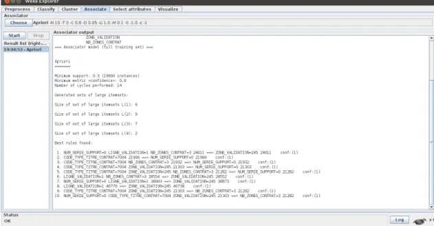
5.8 The Association rules . . . 36

5.9 The Experimenter tool . . . 37

6.1 The histogram of all the attributes . . . 43

6.2 The discretization filter application . . . 44

6.3 The final result of the PreProcess phase . . . 44

9.1 Circled the clusters discovered . . . 82

A.1 The full database parameters description (1) . . . 92

A.2 The full database parameters description (2) . . . 93

(11)

(12)

Chapter 1 Introduction

Recently the digitization of those services managed by the public admin-istration has become a very important aspect in its process of innovation and development.

In this context, a few years ago the Emilia-Romagna Regional Government initiated a project in order to create a general system capable of unifying all single private transport companies under a unique control system.

The final decision was to develop a generalized system.

This would enable passengers to purchase a singular ticket that could be used for buses and trains across all the various operators.

The application of one broad system would pose some crucial questions. The first of which being:

How do we re-distribute the revenue from tickets sales to the single operators, in accordance to their incurred costs?

It would be necessary to implement a clearing system. Designed to compute all the economic evaluations based on the data generated by the operators. Of course, in order to implement this system, operators need to be capable of registering by the appropriate digital device. By their own means the op-erators would log all of their activities. Such as:

Ticket sales, their obliteration, record of time, location, etc.

This data would then be stored and managed by the clearing system. Which

(13)

4 1. Introduction

in turn generates the problem of data security. A suitable clearing system must be able to guarantee that the privacy of all its users is preserved. Also, in consideration of a competitive environment, the computation of the special economic evaluations must not benefit any one the operators over another.

The thesis focuses on the overall analysis of the clearing system, and aim to discover and identify various potential threats and weaknesses to its security.

My objectives in this thesis are:

1. To discuss the development of this project, initiated by Emilia-Romagna Regional Government.

2. To research and implement data mining tests on the database provided. The purpose is to discover patterns and information that may otherwise be hidden.

3. Using the information in these forms we will simulate various privacy attacks. These scenarios will include attacks carried out not only by external vectors, but also from the respective transport operators them-selves.

This scheduling is also the result of discussions after a state of the art phase about data mining and the usage of a software called WEKA; which has been our choice to provide the data mining tests.

At the explicit request of E.R. government the project will be based on an already existing project developed by the business company StartRomagna [25], in 2009 like a fusion of three local business companies of three different areas (Rimini, Forli, Cesena), and now works in this little part of the E.R. Region.

(14)

Chapter 2 System structure

In this chapter we will look into the clearing system’s structure. Particu-larly we will highlight some weaker points in its security, and further outline some developmental aspects.

2.1 Requirements

The clearing system must allow for the integration of relevant data from the operators under a single collection system. This allows appropriate access to involved operators.

Five fundamental security principles this system respects are:

Confidentiality: The restriction of the content. Insuring that information is accessible only to the correct users.

Availability: The service must always be available. With authorization and consistent verification of the supporting parties.

Authorization: Verify the consistence of the supports

Integrity: With the highest levels of assurance that the Data is authenti-cated and has not been modified.

(15)

6 2. System structure

Non-repudiation: The safeguard, non-repudiation, is a crucial aspect of all results.

System structure must be respected by all of its components. Including the message exchange.

Another important system requirement is that the reproducibility of its op-erative results will be preserved. This particular bureaucratic requirement is an essential element. The system must retain the ability to prove previous results of any particular economic evaluation.

The technique used in achieving this, is what we refer as a snapshot. The snapshots are an instantaneous representation, using a portion of the clearing system’s database.

All the economic evaluations will be done through this snapshot. Every snap-shot is saved and encrypted with its meta information along with its hash result in order to guarantee that it will not be modified or deleted in the future.

At a later point, we will further discuss these details in more depth.

2.2 Architecture

The clearing system is based on the distributed architecture composing its different parts. Operators are only responsible for the management and maintenance of their own data. This data is then needed for computation. In a single processing centre it is collected in order to avoid disturbing pro-duction systems of the operators.

The processing centre represents the clearing system. The database is com-posed of the operators input data.

It is necessary for the computation of the information to use the system’s back-end directly. Users have direct access to the front-end of the clearing system via interface to compute economic evaluations.

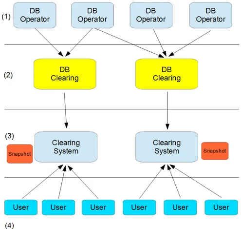
In figure 2.1 we can see the block structure of the system:

(16)

opera-2.2 Architecture 7

Figure 2.1: The clearing system architecture structured in 4 different levels

tors. This is where all the entries are constantly updated. The feeding system collects data periodically between all the databases of the oper-ators concerned. The acquisition is performed using simple SQL query to the second level. At this stage it is important to ensure security during communication using the appropriate VPN.

2. At the second level we have the database clearing, this collects only the information needed clearing. The data collected is filtered at its origin to allow data that does not affect the system to exit the individual operator.

(17)

snap-8 2. System structure

shots on a local database, with the data required to compute the clear-ing functions.

4. The final users access the front-end to compute economic evaluations.

2.2.1 Creation and management of the snapshots

To maintain the consistency of data, a snapshot, once it is created, it cannot be changed. This snapshot is immutable over time. Even if the basis of the original data clearing changes, the snapshot itself cannot.

To ensure this property remains together with the snapshots the following elements are saved and hashed:

• A generic description of the snapshot data for unique identification. And a description of the parameters used to create it.

• The specified users, roles and permissions. The origin of the created snapshot and the users or roles that have access and permissions.

• A time-stamp. Recording dates and times. Start and end.

• Data filters to limit the samples taken, only to the relevant portions of the overall data.

• For security, this being a description of the keys used for data encryp-tion or digital signatures. This will digitally sign the snapshot at the time of its rescue.

Once the snapshot has been created, it is immediately saved as a file along with the safety systems required. Then the snapshot can be restored, or the stored data can be used on the file system.

The snapshots are saved and digitally signed to prevent unauthorized modi-fication of the data.

Each snapshot maintains specific permissions to restrict access. This is to prevent unauthorized use of information.

(18)

2.3 The clearing functions 9

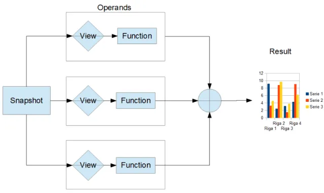
Figure 2.2: The structure of the algorithm of the clearing function

2.3 The clearing functions

Systems that create clearing functions are composed of different elements. These are administered both locally and globally to each and all operators. The purpose being that functions may be available to the different operators. This allows the investigation of the data, including the economic and clearing elements.

Of which may be sold, worn or obliterated.

The system of functions is made up of modules. These modules are to be programmed and then run, for the processing of clearing operations [2]. Each part or module represents a single computational step in which a system is

(19)

10 2. System structure

created.

It is this that allows the investigation of the clearing rules.

Generally, the creation of clearing operations framework consists of logical components shown in 2.2.

Each operation is broken down into different operands. The interpolation algorithm, in the different operands, produces the result of the clearing op-eration. The starting point of each operation is a snapshot that represents a portion of the imported data from the database operators.

Resulting from the clearing operation, the input and output data is repre-sented by the snapshot. This is reprerepre-sented in tabular form.

The clearing operations consist of the following components: [2] • Operand

• View • Function

In any given clearing operation, the operand consists of a view and a function. The clearing operations are algorithmic interpolations of one or more operands. Each operand is characterized by the following components stored on the database containing the relevant permits.

The operands need a formal description. This must define the crucial details of input and output data, the permissions, the users and the roles. This formal description is necessary to enable the identification of data in the formalization of the clearing operations.

The view is a portion of the snapshot data. This filters the input data and returns a representation of the processed input data, functional to the operand.

It is defined by the input data, as the snapshot returns the result in tabular form. It is an SQL query to be applied by a snapshot, which returns a portion of the input data as a tabular representation. The view is used to filters the data source, this must be applied to a function. Which then calculates the

(20)

2.3 The clearing functions 11

operand.

Because these are planned within the database administrator, there is no way to create or modify a view from the software interface. The functions of the operands, access the second view of the permission set. The view of an operand returns, in tabular form, a portion of the snapshot Data, to which it applies a function constituted by a series of algorithmic operations to the input data.

The function is an algorithm. When applied to the view it defines the output of the operand. The function must have the following characteristics:

• Access to local and global parameters of the system

• Must be stored within the database associated with an operand and its permissions.

• Must be programmed, with a programming language, capable of de-scribing cycles and operations. Including conditional access as well as selectively viewed data.

(21)

(22)

Chapter 3 The Stimer’s database

description and the objective of

our work

3.1 The database

After discussing the system’s composition, we should now look into the chosen solution and the data itself. The database is at the fundamental heart of this work, particularly its composition.

The goal of the Stimer’s Project is to track every instance of public transport. Obviously, the system will track all available information about the individual obliterations of each user.

Which can be seen in relation these contracts: [2]

CODE TYPE TITRE CONTRAT Type of the contract (monthly, weekly, ecc)

NUM CONTRAT Contract position on the support (1 for calypso ecc..)

EXPL PROPRIETAIRE CONTRAT The geographic contract type (re-gional, urban, ecc)

(23)

143. The Stimer’s database description and the objective of our work

There are many indeed parameters regarding the relative information. These pertaining to the single use ticket holder are discussed in terms of a contract:

CODE PROFIL USAGER User profile (student, ecc)

DEV PROFIL USAGER Date user profile

NUM SERIE SUPPORT ID of the contract.

But most importantly, we have plenty of relevant information regarding the trace and exact locations of the user. Including the ticket, the validation zone and the purchasing zone etc. For example:

LIGNE VALIDATION The Bus Ligne where the ticket has been vali-dated.

NB PASSAGERS VALIDATION The number of possible transshipments.

NB ZONE VALIDATION The number of zone where the ticket it’s valid.

ZONE VALIDATION The zone where the ticket it’s validated.

SS LIGNE VALIDATION The sub type of the zone. SENS VALIDATION The direction of the travel.

The Appendix will contain a detailed description of the database, includ-ing parameters and attributes.

3.2 Our work

In this section we want to explain what is the goal of our work and his motivation. We saw what would be the final goal of the Stimer’s project; create a clearing system that incorporate all the public transport operators of the Emilia-Romagna Regional Government.

(24)

3.2 Our work 15

hardware and various software problems.

As our topic of discussion is software, it is impossible to ignore the systemic security issues that arise. Considering bulk amounts of private data are being managed. The aspects of crucial importance would be:

• Are the means of this data management secure?

• Is it possible to break the security defences and violate the company’s privacy?

• Should we place more focus on companies rather than single users?

As showed in the figure 3.1 systems such as these have two possible security attack vectors.

The first one is the classical intrusion of third party in which the data are subtracted from the primary database; but this aspect isn’t our topic. It is perhaps what would be regarded as the second most common attack vector that is the focus of our work. This is called an insider attack. Also referred to as an insider threat. This type of attack arises due to a malicious threat from inside the respective organizations themselves.

This raises the question:

Which means of attack shall we need to contend with? It may be necessary begin with some particular assumptions.

In our case, the organization is a union of the public transport operators. Within this unique system (Stimer), a single passenger, being a ticket holder. Will be referred to as a single company.

The system periodically carries out economic evaluations based on data. This data is derived from the individual operators and then distributed corre-sponding to the profits. Importantly, one should note that the system real-izes these evaluations and not the companies. This is because the individual companies would hold little information in relation to competitors. Of course subsequent information is encoded within the parameters and attributes of the database.

(25)

163. The Stimer’s database description and the objective of our work

This means that the companies cannot know, for example, which is the con-tract type most sold in a certain area, which is instead the most used and so on; information of this nature would be very useful in order to compete. But now, what if a single company try to attack his competitors of the same system?

As attack we get on is possible that single operators, with particular analysis, are able to obtain sensitive information on the work of other companies? Finally we shift to the primary focus of our work.

In this thesis, we aim to demonstrate whether it is possible that by using this system a company can obtain sensitive information revealing the actions of its competitors, and in turn use this information fraudulently.

Consequently, the next question we must answer is: How should we proceed?

Motivated by this subject, in the next chapter we will operate a data mining analysis. With the available data, our analysis will involve tests using the famous data-mining tool called WEKA. Which will be used to provide infor-mation that otherwise should be hidden.

After that we will offer explanations as to how this information can be used. Thus, creating these possible scenarios. Following this we will discuss feasible preventative measures that could be employed for these kinds of attacks. Next, we should look at our chosen strategies.

(26)

3.2 Our work 17

(27)

(28)

Chapter 4 Data Mining in the literature

In the last years we have seen the advent of big data, with the exponential growing of gigabytes of data that were shared all around the world.

Firms, companies and even public administration compete each other in or-der to make the largest possible amount of user information.

The underlining belief now, is that one can know anything, learn any aspect, and discover any detail of our lives through these digital footprints and var-ious profiles.

But what can happen when, thankfully, digital privacy is respected? Or, when we simply cannot access certain information?

A solution to obtaining such information can be data mining.

Data-mining techniques have attracted a great deal of interest from the in-formation industry. In recent years this has also captured the wider interest of a society in general. This is due to the imminent need to transform these huge amounts of data into useful information. With the results of this often leading to far greater knowledge of any given topic.

Many of these gains are immediately applicable, ranging from market anal-ysis, fraud detection, customer retention, production controls and science exploration.

A logical question to ask is: what exactly is data mining? [18] [21]

Data mining is defined as, the process of discovering patterns in data and,

(29)

20 4. Data Mining in the literature

extracting knowledge from large amounts of data. The process must be au-tomatic or, more usually, semi-auau-tomatic.

But what can Data Mining Do? As [3] explained very well although data mining is still in its infancy, companies in a wide range of industries including retail, finance, heath care, manufacturing transportation, and aerospace are already using data mining tools and techniques to take advantage of histori-cal data.

Using technologies that rely on pattern recognition along with statistical and mathematical techniques. The data is processed, essentially sifting through warehoused information.

This data mining helps analysts recognize significant facts, relationships, trends, patterns, exceptions and anomalies that may otherwise have gone unnoticed.

For businesses, data mining is used to discover patterns and relationships in the data. This then helps to make more informed business decisions.

Data mining can help spot sales trends. Thus, being used to develop smarter marketing campaigns and improve accuracy when predicting customer loy-alty. Specific uses of data mining include[1]:

Market segmentation Indication and correlation of the common charac-teristics of customers who buy the same products from a company.

Customer churn This predicts which customers are likely to leave your company and move to a competitor.

Fraud detection Identification of the transactions that are most likely to be fraudulent.

Direct marketing Specifying which prospects should be included in a mail-ing list to obtain the highest response rate.

Interactive marketing Used for predictions of what individuals accessing a web site are more likely to be interested in viewing.

(30)

21

Market basket analysis This aims to increase the understanding of prod-ucts and services that are commonly purchased together.

Trend analysis Reveals the difference between a typical customer, within monthly, quarterly and yearly cycle.

Understanding of data mining in this way directs us to the next question: How could the use of these techniques, or similar, become a security threat to our system?

Firstly, by defining the patterns of hidden information between these companies. Following this, we can decipher the relevant information and devise methods to penetrate the security walls. Making it simple to violate the privacy of user and/or companies. As we’ve previously outlined, data mining is a process. This leads us to ask:

What the relative steps? In fact, the process of data mining will be part of a wider process.

Being, data processing; in which we find a pre-process phase, this will include:

1. Data cleaning: This removes incorrect and null values, referred to noise.

2. Data integration: In which we can unify multiple sources or complete missing data.

3. Data selection: This is where only the relevant values of interesting are selected in accordance the objectives of our analysis.

4. Data transformation: Data may be transformed or consolidated into forms that are appropriate for data mining algorithms. Doing so by performing summary or aggregation operations. Including discretiza-tion, etc.

Next is a test phase. This includes:

1. Data mining: Being the heart of our analysis. Applying intelligent methods and algorithms to then extract data patterns.

(31)

22 4. Data Mining in the literature

2. Pattern evaluation: Involving the interpretation of these results, in order to justify the measurements.

3. Knowledge presentation: Techniques to represent this knowledge, in-cluding visualizations can then present the mined data.

Previously we have been discussing patterns.

So, let’s clarify: What are patterns? During our data mining analysis we have seen that using probabilistic methods and algorithms can determine, or even better predict, the values, parameters and trends using only the subset values. In which case, such patterns are the parameters of prediction, along with association rules in the prediction of trends. In all cases, high quality coefficient would be required.

With reference to the previous chapter:

How was the data mining process used? In this phase we will illustrate how we have discovered patterns in the Stimer’s Database system for public transport operators.

In particular, will describe how such a pattern can be used to derive the information that theoretically should be completely hidden. Of course, this then could be employed as a means to violate the security of the system.

(32)

Chapter 5 WEKA

In this chapter we begin our analysis.

As mentioned previously we choose a very powerful software called WEKA. [16] WEKA is an open source software issued under the GNU General Public License.

”WEKA” stands for the Waikato Environment for Knowledge Analysis, which was developed at the University of Waikato in New Zealand. WEKA like ev-ery open-source project it’s freely downloaded, and it’s written in Java, so it could runs on almost every platform.

To further specify: what is WEKA?

WEKA is a collection of machine learning algorithms for data mining tasks written in Java.

The algorithms can either be applied directly to a dataset or called from your own Java code. WEKA contains specific tools for every data mining step that we have discussed; tools for data pprocessing, classification, re-gression, clustering, association rules, and visualization.

WEKA is used for research, education, and applications. Among the various choices at our disposal, we focused on WEKA because gathers a compre-hensive set of data pre-processing tools, learning algorithms and evaluation methods, graphical user interfaces (incl. data visualization) and environment for comparing learning algorithms. [5]

(33)

24 5. WEKA

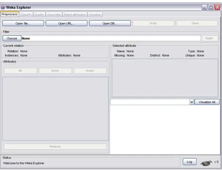
In order to better understand the usage of WEKA we will see a practical example of the WEKA’s structure. The Gui shows in 5.1 the possible appli-cations that we have:

Figure 5.1: The WEKA GUI Interface

The buttons can be used to start the following applications:

Explorer An environment for exploring data with WEKA (Almost all the work was done with this application)

Experimenter An environment for performing experiments and conducting statistical tests between learning schemes and to compare the results of the algorithms

KnowledgeFlow This environment supports essentially the same functions as the Explorer but with a drag-and-drop interface.

SimpleCLI Provides a simple command-line interface that allows direct ex-ecution of WEKA commands for operating systems that do not provide their own command line interface.

(34)

5.1 Explorer 25

5.1 Explorer

The Explorer application is the most important. It has been a center from which to base our work. And it is where all the WEKA functions have been developed.

As you can see on the picture 5.2 the explorer GUI is divided in six tabs: PreProcess, Classify, Cluster, Associate, Select attributes, Visualize.

Figure 5.2: The WEKA GUI Explorer Interface

5.1.1 PreProcessing

Firstly, we must of course upload our dataset. At this stage we have multiple options. These are:

1. To open a file containing our data the description. This could be a csv file, an arff (the WEKA data type) or even sql.

2. Open from a URL where the resource data is located.

(35)

26 5. WEKA

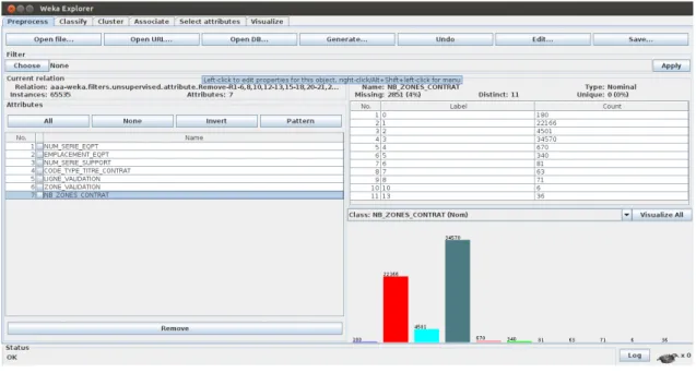
Once our data has been loaded we can start the pre-process phase using the pre-process panel. This shows a variety of information.

As shown in picture 5.3 there is a currently loaded data box that has three entries:

Relation This names the relation, as given in the file it was loaded from. Filters (described below) modify the name of a relation.

Instances The number of instances (data points/records) in the data.

Attributes The number of attributes (features) in the data.

Of course in this step we should work with the attributes, modifying them with all the techniques described in the next chapter.

Below the Current relation box there is a box titled Attributes, where can find a list of the attributes:

No A number that identifies the attribute in the order they are specified in the data file.

Selection tick boxes These allow you to select which attributes are present in the relation.

Name The name of the attribute, as declared in the data file.

When you click on different rows in the list of attributes, the fields change in the box to the right titled Selected attribute. This box displays the char-acteristics of the currently selected attribute in the list:

Name The name of the attribute, the same as that given in the attribute list.

Type The type of attribute, most commonly Nominal or Numeric.

Missing The number (and percentage) of instances in the data for which this attribute is missing (unspecified).

(36)

5.1 Explorer 27

Distinct The number of different values that the data contains for this at-tribute.

Unique The number (and percentage) of instances in the data having a value for this attribute that no other instances have.

Below the statistics is a list. This displays more information about the values stored in this attribute, differing depending on their type. If the at-tribute is nominal, the list consists of each possible value for the atat-tribute along with the number of instances that have that value.

If the attribute is numeric the list will give four statistics describing the dis-tribution of values in the data. These are: The minimum, maximum, mean and standard deviation.

And below these statistics there is a colored histogram, color-coded accord-ing to the attribute. Which is chosen as the class, usaccord-ing the box above the histogram. This box will bring up a drop-down list of available selections when clicked.

Finally, after pressing the visualize all button, histograms for all the at-tributes in the data are shown in a separately unless, as in our case, there are attributes with too many values to show.

Returning to the attribute list in the picture 5.3 it should be noticed that there are three buttons that can also be used to change the selection: All All the boxes become ticked.

None All the boxes are cleared (un-ticked).

Invert This changes ticked boxes to become un-ticked boxes. And vice versa.

Once the desired attributes have been selected, they can be removed by clicking the Remove button below the list of attributes.

The last important option of the PreProcess application is that we can ap-ply PreProcess algorithms by simap-ply choosing one from the filter bar; choose

(37)

28 5. WEKA

the attributes and click to apply on the right corner, and after that the Pre-process panel will then show the transformed data.

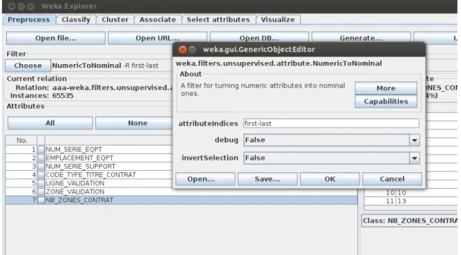
Here there is an important observation to make. It is possible to set up some parameters and the value of this algorithm. This is done on the filter bar after choosing the filter algorithm.

It is possible to see an example of the numeric to nominal filter shown here in picture 5.4.

Figure 5.3: The WEKA PreProcess tab with the data loaded

5.1.2 Classify

The second, and most important, application that we used is the classify tab; the one on which we will do some experiments with the data mining algorithms.

At the top of the classify section we have the Classifier box. This box has a text field that names the currently selected classifier and its options. When selecting a classifier you have also the opportunity to choose many filters or different parameters that will be used in the tests. The result of applying

(38)

5.1 Explorer 29

Figure 5.4: The filter Numeric to Nominal application on the dataset

the chosen classifier will be tested according to the options that are set in the Test options box. We have three Different choices with which to test our data with the classifier.

These choices are the following:

Use training set The classifier is evaluated on how well it predicts the class of the instances it was trained on.

Supplied test set The classifier is evaluated on how well it predicts the class of a set of instances loaded from a file.

Cross-validation The classifier is evaluated by cross-validation, using the number of folds that are entered in the Folds text field.

Percentage split The classifier is evaluated on how well it predicts a certain percentage of the data which is held out for testing.

The amount of data in the percentage is split into the number of folds, and so on. Here we can also see there is an influential parameter for the results.

(39)

30 5. WEKA

Once we know how to launch the algorithms, we need to know what we will search for.

The classifiers algorithms implemented in WEKA are designed to predict a single ”class” attribute, that is to say a single parameter, which is the target for prediction.

In terms of prediction, there are numerous differences. This is because some classifiers only learn nominal classes, whereas, others can only learn numeric classes. An example is linear regression. Then there are others that can learn both.

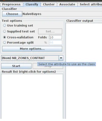
By default, the class is taken to be the last attribute of the data. But if you want to set the classifier in order to predict a different attribute, they may be chosen from the box below the test options box.5.5

Once the classifier, the test options and class have all been set. Finally the learning process can start, by simply clicking on the Start button. The classifier output area to the right of the display is filled with text de-scribing the results of training and testing. A new entry appears in the result list box. We can look at the result list below. But first we try to understand the output text.

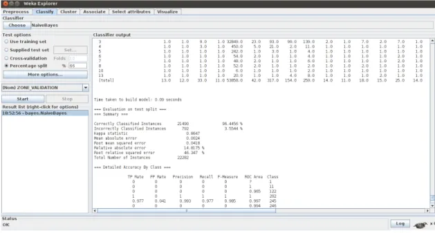
The text in the classifier output area allows you to browse the results. The most important thing to notice here is that the text output is divided in several parts. Each one will represent particular information:

• Run information. A list giving the learning scheme options. Including the relation name, the instances, the attributes and test mode that were involved in the process.

• Classifier model (full training set). This is a textual representation of the classification model that was produced from the full training data. • The results of the chosen test.

• Summary. This is a list of statistics summarizing how accurately the classifier was able to predict the true class of instances under the chosen test mode.

(40)

5.1 Explorer 31

• Detailed Accuracy By Class. A more detailed per-class breakdown of the classifier’s prediction accuracy.

• Confusion Matrix. This will show how many instances have been as-signed to each class.

Finally we should be able to have a good representation, and storage of the results. As there are many different choices [20] picture 5.6:

View in main window This shows the output in the main window (left-clicking the entry).

View in separate window This opens a new independent window for view-ing the results.

Save result buffer This will bring up a dialog allowing you to save a text file containing the textual output.

Load model This loads a pre-trained model object from a binary file.

Save model This saves a model object to a binary file. Objects are saved in Java ’serialized object’ form.

Re-evaluate model on current test set This takes the model that has been built and tests its performance on the data set that has been specified with the set button under the supplied test set option.

Visualize classifier errors This opens a visualization window that plots the results of the classification. The correctly classified instances are represented as crosses. Whereas, incorrectly classified ones are shown as squares.

Visualize tree or Visualize graph This opens a graphical representation classifier models structure, when possible (i.e. for decision trees or Bayesian networks). The graph visualization option only appears if a Bayesian network classifier has been built. In the tree visualizer you

(41)

32 5. WEKA

can bring up a menu by right-clicking a blank area. Then, pan around by dragging the mouse seeing the training instances at each node, by clicking on it. CTRL-clicking zooms the view out, while SHIFT- drag-ging a box zooms the view in. Basically, the graph visualizer should be self-explanatory.

Visualize margin curve This will generate a plot illustrating the predic-tion margin. The margin is defined as the difference between its prob-abilities, as predicted for the actual class, and the other class’s highest probability prediction.

For example:

Boosting algorithms may achieve a better performance on test data by increasing the margins on the training data.

Visualize threshold curve This generates a plot illustrating the tradeoffs in a prediction that is obtained by varying the threshold value between the classes.

For example:

With a default threshold value of 0.5. The predicted probability of a positive must be greater than 0.5, for this prediction to be positive. The plot can be used to visualize the precision/recall tradeoffs. For ROC curve analysis (true positive rate opposed to false positive rate), and for other types of curves.

Visualize cost curve The plot that is generated gives an explicit represen-tation of the expected cost.

5.1.3 Clustering

Looking to the second tab, we find the Cluster application.

The cluster mode box is used to choose the cluster, and the evaluation of the results.

(42)

5.1 Explorer 33

Figure 5.5: The possible options for the dataset on the classification tab

set, Supplied test set and Percentage split.

In these, the data is assigned to clusters instead of trying to predict a specific class.

The fourth mode is the Classes to clusters evaluation. This makes a com-parative assessment of how the chosen clusters match the pre-assigned data class.

There is an additional option in the Cluster mode box. This is the Store clusters for visualization tick box. This determines whether or not it will be possible to visualize the clusters once training is complete. When dealing with these large datasets, computational memory and processing power can become a real problem. To manage this it may be helpful to disable some options. Unfortunately, this can often be the case. This being so, some attributes in the data should be ignored when clustering. It is the ignore attributes button that will open a small window allowing for the selection of which attributes to ignore.

(43)

34 5. WEKA

Figure 5.6: The Classification output

Why should we ignore some attributes? The various motivations can be:

1. The number of instance are so many that it is impossible to make cluster analysis on the whole dataset; this is why someone must be eliminated.

2. There is not enough distance in the clustering to determine the clusters of interest. This being so, we must restrict our dataset.

3. There are many attributes that are not of interest, due to redundancies.

Once the cluster algorithm is selected, we can enter the correspondent parameters. Next is the percentage split (the dataset) and then launch the application. It is then time to manage these results.

The cluster section, like the classify section, has Start/Stop buttons. It has a result text area and a result list. These all behave like their classification counterparts.

Right-clicking an entry in the result list brings up a similar menu, except that it shows only two visualization options: Visualize cluster assignments

(44)

5.2 Experimenter 35

and visualize tree which opens other windows all where the cluster graphics are shown.5.7

5.1.4 Associating

The second panel of the explorer application is the association panel. This panel contains schemes for learning association rules. These learners are chosen and configured in the same way as the clusters, filters, and classifiers in the other panels.

As we have previously noted, we only need to choose the association algo-rithms that we want to use, and sets the parameters. Then finally the results, in particular the association evidence is shown on the right panel of this tab. The rules are easy to understand. To better understand this, we could draw a mental picture of this being a series of nested statements. Resulting with a certain correctness coefficient.5.8

5.2 Experimenter

Lastly, the second application we have used is called the experimenter. Once we have completed our numerous analyses, and compared the results with the algorithms. The experimenter is very useful when comparing the efficiency of different algorithms.

The experimenter operates by combining the launch of two different classi-fiers, directly outputting the result of its comparison.

As displayed, on image 5.9, once the dataset is loaded and the experiment type is specified (cross fold, percentage split), we can set the algorithms that are to be compared. These are added singularly in the relevant box in the tab.

We can now save this model to launch the analysis. In the relevant tab the file containing our configuration can be loaded. Then the algorithm compar-ison process can start. In the right box the results are shown, each algorithm is evaluated with a efficiency coefficient, here we can see the differences.

(45)

36 5. WEKA

Figure 5.7: The Cluster analysis

(46)

5.2 Experimenter 37

(47)

(48)

Chapter 6 Pre-Process phase

In this chapter begins the description of work that is central to the thesis. Given that we have our database and our data WEKA mining software. How should we then wish to proceed? To initiate our analysis we first start the pre-processing of data. Preprocessing phase consists of manipulation and transformation of data before to applying the data mining algorithms. This transformation is made using several techniques that will be applied either manually or directly on the dataset, or, through some WEKA filters.

Why is this step necessary? Fundamentally there are two reasons:

1. Firstly because our data may be ‘dirty’. This can mean that the data is incomplete, inconsistent or incorrect. This then will need the cleaning step. [10]

2. Secondly, we will apply the data-mining algorithm. As we have a huge amount of data and the algorithms are quite complex. In order to improve the performance of the algorithm and, thus, our result, we need to implement some algorithmic pre-process transformation such as discretization or categorization. These algorithms act to rearrange the data with specific criteria. We can illustrate that WEKA can help us in this.

(49)

40 6. Pre-Process phase

6.1 Elimination

The first, and rather simple analysis shows us that some of the attributes do not have a useful range of possible values for us. As seen in picture 6.1 there are 23 further examples of this, although. These do have a broad range of possible values. Typically over 100, these represent only few of them (less than 2). When the values are not useful we need to create association rules. Attributes with too fewer values can be indicative that we do not have enough differences. More than 99% of the attributes instances are represented only by a single value. We have decided to completely eliminate these attributes.

6.2 Missing

Some of the attributes have shown large proportions of missing data. This problem can be managed in two different ways, in turn leading to two different interpretations of the results.

1. We can add a category that incorporates all the empty values. Using this as a new nominal value.

2. We can replace the empty values with a possible trend that statistically reflects the values already present. Done in such a way that the general distribution is not altered.

In the first solution shown we do not change the values. Since it is as if we were creating a new possible nominal value during the creation of the association rules. We could have false positives in many of these cases. Regarding the second solution, we can see that by adjusting the values and introducing a coefficient error during the classification and association pro-cess can, in some cases, be tolerable.

We found it is suitable to use this solution without large quantities of empty values, when there were, we had decided to use the first solution.

(50)

6.3 Incorrect 41

6.3 Incorrect

Using the same principle even in a case where we had detected the incon-gruence from certain values. In particular, not corresponding to the type of parameter. Here we decided to use the previous techniques.

6.4 Categorization

Another important technique that we used is called categorization.[23] Categorization is a part of cognition and is fundamental to the process of comprehension. Categories play a central role in perceptions, learning, com-munication and thinking. Categorization is used to group objects together into classes, based on similarities. These classes are called categories or con-cepts.

Group values under different categories are very important. Without these, every object or incidence would appear inimitable. Hence, there would be no way to predict new unknown objects. Thus, categories can be seen as a product of interactions, and can help us in the performance result.

There are many techniques of categorization. Most of these are aimed to build knowledge.

What we have used is the classical sense, is that claims that have categories are discrete entities. These are characterized by a set of properties and shared by their members. These properties assume the established condi-tions. These are necessary and need to be succinct in order to capture the meaning of a category.

Within these conditions our example is divided into some attributes such as the Code Type Titre Contract attribute. This division could be compared to a triage process, depending on three macro categories. Which are already described in [2]; where the contract are considered as:

• Contratto Ordinario Corsa Semplice

(51)

• Carta Valore Corsa Semplice

• Carta Valore Multicorsa

6.5 Discretization

Some of the algorithms that we used to create data mining models in WEKA, required specific content types in order to function correctly. An example of this is the Naive Bayes algorithm. This cannot use continuous columns as input and cannot predict continuous values. Additionally, some columns may contain so many values that the algorithm cannot easily iden-tify its patterns of interest in the data from which it creates a model. In these cases, you can discretize the data in the columns to enable the use of the algorithms that produce a mining model.

Discretization is the process of putting values into buckets so there are a limited number of possible states.

The buckets themselves are treated as ordered and discrete values. You can discretize both numeric and string columns.

There are several methods to use when discretizing data.

Fortunately, all this methods are present in the WEKA pre-process tool. This operation can be applied by the use of a filter, consisting of this dis-cretization method.

We can demonstrate these methods, and the data we have used.

Basically the discretization learning methods are divided in two categories. These are supervised and unsupervised.

As defined in [9]: Supervised learning is also often referred to as directed data mining.

In this method, variables under investigation can be split into two groups. And these are explanatory variables and one or more dependent variables. The target of the analysis is to specify a relationship between the explanatory variables and the dependent variable as done in the regression analysis. To apply directed data mining techniques the values of the dependent variable

(52)

6.5 Discretization 43

must be known for a sufficiently large part of the data set.

Otherwise, the unsupervised learning is closer to the exploratory split of data mining. In unsupervised learning situations all variables are treated in the same way. There is no distinction between explanatory and dependent vari-ables. In contrast to its name, undirected data mining does have a target to achieve. This target might be as general as data reduction, or specific, such as clustering.

Supervised learning requires the target variable to be well defined and that a sufficient number of its values are given. Unsupervised learning typically has either the target variable as unknown. Or it has only been recorded for small a number of cases.

Despite the apparent complexity of this method, WEKA offers us a pow-erful filter in the pre-process tab. This allows us to compute both types (supervised and unsupervised) of discretization filter. Shown in picture 6.2 the discretization filter application is in our dataset. In picture 6.3 the final result of the pre-process phase with the WEKA tool is shown.

(53)

Figure 6.2: The discretization filter application

(54)

Chapter 7 Data Mining Algorithms

The pre-process step is done in preparation for submitting data to the data-mining algorithms, implemented by WEKA.

The questions to be asked here are:

Which algorithms, and how do they work? [3] [8]

Within this chapter we will show the data mining algorithms that have been used. Here we have used three fundamental classes of algorithm.

7.1 Clustering

Within this context, the use of the word clustering and the term cluster analysis was introduced by Robert Tryon in 1939. Clustering or cluster anal-ysis is a set of techniques for multivariate data analanal-ysis that aims to select and group homogeneous elements in a data set. The goal of these algorithms is grouping the items based on a relative measurement of similarity.

This measurement is called distance. The technique, after the identification of a group, will insert each element in each group according to its distance. The measurement and the distance threshold give the accuracy of the al-gorithm; this is an input factor in each group. In turn, these clustering algorithms are divided according to two approaches.

These approaches are:

(55)

46 7. Data Mining Algorithms

Bottom-Up: In this, the elements are considered as clusters themselves. Then the algorithm proceeds to unify the nearest cluster until a fixed minimum number of clusters is reached. Or, when the minimum dis-tance between clusters does not exceed a certain value.

Top-down: This approach begins with a unique large cluster containing all the elements. Within algorithms there are provisions that divide this cluster and in turn create others according to a distance value, until a termination condition is reached. As an example, this could be a fixed number of clusters.

In order to find the clusters of interest in our analysis we have used a famous algorithm called K-Means. We have relied on WEKA’s explorer tool to implement this.

The algorithm K-Means is a clustering algorithm, which allows the partition to divide a set of objects into K groups based on their attributes.

With clustering partition (also called non-hierarchical) we define the mem-bership of a group by a distance from the point representative of the cluster (centroid, etc.).

Having fixed the number of groups in the partition result, it is then a variant of algorithm expectation-maximization (EM) that has the objective to deter-mine the K sets of data generated by Gaussian distributions. It is assumed that the attributes of the objects can be represented as vectors. Thus, form-ing a vector space.

In a nutshell, the purpose of this algorithm is the following: [12]

Each cluster is identified by a centroid or middle-point. The algorithm fol-lows an iterative procedure. First of all it creates K partitions and assigns at each partition an entry point.

This is done so in a random way or by using some heuristic information. It then calculates the centroid of each group, and constructs a new partition as-sociating each entry point to the cluster whose centroid is the closest. Then the centroids are recalculated for the new cluster. This process continues until the algorithm converges.

(56)

7.2 Decision trees 47

Why did we choose this algorithm? Our reasoning here is that this algorithm may have a more suitable convergence time, with particular parameters. Par-ticularly, when there is not too much partitioned data.

This is true in our case, as stated we have approximately only 7 relevant attributes. As we have chosen the number of clusters we want to find in advance, this algorithm will converge very quickly. In our case, we found this to be true. Even with massive amounts of data.[7]

7.2 Decision trees

The decision tree is a graph model of decisions and the possible conse-quences.

In data mining decision trees are used to classify data, as in fact, they are also referred to as classification trees.

This type of graph can describe a decision structure, where nodes may rep-resent the instance classification. And the ramifications reprep-resent the prop-erties that lead to these classifications.

The leaves, of the tree, will be the final classes of the various decisions that are made within the classification process.

In this tree, as explained in [24] there are two fundamental conditions:

The split condition: This condition is the predicate that is associated with each internal node. This takes place in the beginning where the data is distributed.

The terminal condition: This identifies the maximum depth of the tree. Contrary to what one may initially assume, increasing the depth of this tree, essentially makes the model more complex. Will not always a have a beneficial result.

The decision tree we have used is the C4.5 algorithm. In the WEKA program this is implemented with the name of J48 (Java version) found in the classification tool.[19] C4.5 is an algorithm used to generate a decision

(57)

48 7. Data Mining Algorithms

tree that was developed by Ross Quinlan. This in particular is an extension of Quinlan’s earlier ID3 algorithm. The decision trees generated by C4.5 can be used for classification. For this reason, C4.5 is often referred to as a statistical classifier. For this reason, WEKA’s team have chosen to implement a java version of his tools.

As described in [11] C4.5 builds decision trees from a set of training data using the concept of information entropy. The training data is a set of pre-classified samples. Each sample consists of a P-dimensional vector. This is where they represent attributes or features of the sample, as well as the class it may fall into.

At each node of the tree, C4.5 chooses the attribute of the data that most effectively splits its set of samples into subsets, enriched in the respective classes. The splitting criterion is the normalized information gain (difference in entropy). The attribute with the highest normalized information gain is chosen to make the decision and the C4.5 algorithm then recurs on the smaller sub-lists.

7.3 Probabilistic Classifier

As the name suggest they represent a probabilistic approach to solving classification problems. [4] Unlike decision trees, in this case it determines within a certain probability, the membership of an object to a particular class. Given a sample input, the probabilistic classifier is able to predict a probability distribution over a set of classes, rather than only predicting a class for the sample.

Probabilistic classifiers provide classification with a degree of certainty, which can be useful when combining them into larger systems.

Basically the probabilistic classifiers fall into two broad categories. Some models such as logistic regression are conditionally trained.

This means that they optimize the conditional probability directly on a train-ing set. Whereas, some models such as Naive Bayes, which we will use, are

(58)

7.3 Probabilistic Classifier 49

trained generatively. Meaning that when the class-conditional distribution and the class prior are found, the conditional distribution is derived using Bayes’ rule, at the time of training.[6] [17]

In our analysis we used the most famous Naive Bayes Algorithm.

The Bayesian Classification represents a supervised learning method as well as a statistical method for classification. It assumes an underlying proba-bilistic model and it allows us to capture uncertainty about the model in a principled way by determining probabilities of the outcomes. It can solve diagnostic and predictive problems.

This Classification is named after Thomas Bayes (1702-1761), who proposed the Bayes Theorem.

Bayesian classification provides practical learning algorithms where prior knowledge and observed data can be combined.

Bayesian Classification provides a useful perspective for understanding and evaluating many learning algorithms. It calculates explicit probabilities for hypothesis, and is robust in its tolerance of noise in its input data.

Why did we choose the Naive Bayes Algorithm for this analysis? This model is simple for us to build. It is an algorithm without complicated iterative pa-rameter estimation. So this is particularly useful in very large datasets, which the case in our analysis. Despite its simplicity, the Naive Bayesian classifier often does surprisingly well. It is widely used because it often outperforms more sophisticated classification methods.

(59)

(60)

Chapter 8 The test phase

Finally, we can proceed to the test phase.

As we have our data pre-processed, our algorithms, and our data mining tools, we can make our analysis. The analysis follows the WEKA organiza-tion. To begin with, we will provide some classification analysis, following this we will search for cluster results. Then finally we will discover some association rules.

For each step and each result, we continue to make improvements. This af-fects the result of the algorithm changing its input dataset. By this we are referring to the re-application of these pre-process techniques.

We will confirm the results using different algorithms that have the same purpose. The structure of this chapter will follow on from this notion. We will dedicate section for each experiment.

And each of these experiments will include:

Attribute to use As covered previously, for various reasons, we will not use all the attributes. In each instance we will choose a set of different attributes. Although, since the quantities of useful attributes aren’t too high. We should find some possible combinations that are particularly fruit-full.

Attribute to predict This objective is the prediction of a single value that should be understandable, theoretically. Of course not every attribute

(61)

52 8. The test phase

is a good candidate for our purpose. Therefore, we should proceed only with attributes deemed to be of real interest to us.

And of course, it is important to remember. The more interesting we find these attributes to be, the more dangerous they are. Because potentially, these may be utilized, becoming a threat to our system.

Algorithm For each technique we appropriate an algorithm. In many cases we use different tests for different settings of the algorithm

Dataset For each test we need to set the dataset input, according to what the data-mining algorithm learns.

8.1 Classification Tests

The first, and most important tests we provide are the classification tests. With some classifiers, the algorithm aims to predict a certain attribute, using a subset of our dataset that is pre-processed. Our aim here is to guess a value. Therefore, the value of output that we need to pay most attention to is the Correctly Classified Instances percentage.

And, where it is possible, the Detailed Accuracy By Class.

Test 1

Configuration Input:

Algorithm Naive Bayes

Attributes input (NUM SERIE EQPT, EMPLACEMENT EQPT, NUM SERIE SUPPORT, CODE TYPE TITRE CONTRAT, LIGNE VALIDATION, ZONE VALIDATION,

NB ZONES CONTRACT)

Dataset Percentuage split 50.0%

(62)

8.1 Classification Tests 53 Text output: === Run information === Scheme:weka.classifiers.bayes.NaiveBayes Relation: aaa-weka.filters.unsupervised.attribute.Remove-R1-6, 8,10,12-13,15-18,20-21,23-29-weka.filters.unsupervised.attribute. NumericToNominal-Rfirst-last Instances: 65535 Attributes: 7 NUM\_SERIE\_EQPT EMPLACEMENT\_EQPT NUM\_SERIE\_SUPPORT CODE\_TYPE\_TITRE\_CONTRAT LIGNE\_VALIDATION ZONE\_VALIDATION NB\_ZONES\_CONTRAT

Test mode:split 50.0% train, remainder test

Time taken to build model: 0.04 seconds

=== Evaluation on test split === === Summary ===

Correctly Classified Instances 27701 84.5393 % Incorrectly Classified Instances 5066 15.4607 % Kappa statistic 0.2363

Mean absolute error 0.0002 Root mean squared error 0.0104 Relative absolute error 51.6412 % Root relative squared error 85.7945 %

(63)

Total Number of Instances 32767

This prediction could have a high level of positive results. In this case we believe we can improve them even further.

So we continue to perform the same test on the same prediction attribute but we change some parameters.

Test 2

NB ZONES CONTRACT)

Dataset Cross-validation 10 folds

Attribute to predict NUM SERIE SUPPORT

Text output: === Run information === Scheme:weka.classifiers.bayes.NaiveBayes Relation: aaa-weka.filters.unsupervised.attribute.Remove-R1-6,8, 10,12-13,15-18,20-21,23-29-weka.filters.unsupervised.attribute. NumericToNominal-Rfirst-last-weka.filters.unsupervised.attribute.Remove-R5 Instances: 65535 Attributes: 6 NUM_SERIE_EQPT EMPLACEMENT_EQPT NUM_SERIE_SUPPORT

(64)

8.1 Classification Tests 55

CODE_TYPE_TITRE_CONTRAT ZONE_VALIDATION

NB_ZONES_CONTRAT

Mean absolute error 0.0002 Root mean squared error 0.0094 Relative absolute error 54.9755 % Root relative squared error 78.2344 % Total Number of Instances 22282

Test 3

NB ZONES CONTRACT)

(65)

56 8. The test phase === Run information === Scheme:weka.classifiers.bayes.NaiveBayes Relation: aaa-weka.filters.unsupervised.attribute.Remove-R1-6, 8,10,12-13,15-18,20-21,23-29-weka.filters.unsupervised.attribute. NumericToNominal-Rfirst-last Instances: 65535 Attributes: 7 NUM_SERIE_EQPT EMPLACEMENT_EQPT NUM_SERIE_SUPPORT CODE_TYPE_TITRE_CONTRAT LIGNE_VALIDATION ZONE_VALIDATION NB_ZONES_CONTRAT Test mode:10-fold cross-validation

=== Stratified cross-validation === === Summary ===

(66)

8.1 Classification Tests 57

Test 4

Algorithm Naive Bayes -D (useSupervisedDiscretization)

NB ZONES CONTRACT)

Text output: === Run information === Scheme:weka.classifiers.bayes.NaiveBayes -D Relation: aaa-weka.filters.unsupervised.attribute.Remove-R1-6, 8,10,12-13,15-18,20-21,23-29-weka.filters.unsupervised.attribute. NumericToNominal-Rfirst-last-weka.filters.unsupervised.instance.Randomize-S42 Instances: 65535 Attributes: 7 NUM_SERIE_EQPT EMPLACEMENT_EQPT NUM_SERIE_SUPPORT CODE_TYPE_TITRE_CONTRAT LIGNE_VALIDATION ZONE_VALIDATION NB_ZONES_CONTRAT Test mode:10-fold cross-validation

(67)

=== Stratified cross-validation === === Summary ===

Test 5

Attributes input All the attributes of the original dataset

Dataset Percentage split 66%

Attribute to predict CODE TYPE TITRE CONTRAT

Text output:

=== Run information ===

Scheme:weka.classifiers.bayes.NaiveBayes

Relation: aaa-weka.filters.unsupervised.attribute. NumericToNominal-Rfirst-last-weka.filters.unsupervised.

(68)

8.1 Classification Tests 59 attribute.Remove-R1-weka.filters.unsupervised.attribute. Remove-R26-weka.filters.unsupervised.attribute.Remove-R3-4,7,17,23 Instances: 65535 Attributes: 23 DTHR_VALIDATION CODE_PROFIL_USAGER SOUS_TYPE_EQPT NUM_SERIE_EQPT EMPLACEMENT_EQPT CODE_TECHNO_SUPPORT NUM_SERIE_SUPPORT TYPE_SUPPORT EXPL_EMETTEUR_SUPPORT CODE_TYPE_TITRE_CONTRAT NUM_CONTRAT EXPL_PROPRIETAIRE_CONTRAT NB_PASSAGERS_VALIDATION LIGNE_VALIDATION SS_LIGNE_VALIDATION SENS_VALIDATION ZONE_VALIDATION TYPE_TRANSACTION NB_UNITE_VALIDATION CLASSE_VALIDATION DTHR_INSERTION DTHR_MODIFICATION NB_ZONES_CONTRAT

(69)

Test 6

Algorithm Naive Bayes -D (useSupervisedDiscretization)

Attributes input All the attributes of the original dataset

Dataset Percentage split 66%

Attribute to predict CODE TYPE TITRE CONTRAT

Text output: === Run information === Scheme:weka.classifiers.bayes.NaiveBayes -D Relation: aaa-weka.filters.unsupervised.attribute. NumericToNominal-Rfirst-last-weka.filters.unsupervised. attribute.Remove-R1-weka.filters.unsupervised.attribute. Remove-R26-weka.filters.unsupervised.attribute.Remove-R3-4,7,17,23 Instances: 65535

(70)

8.1 Classification Tests 61 Attributes: 23 DTHR_VALIDATION CODE_PROFIL_USAGER SOUS_TYPE_EQPT NUM_SERIE_EQPT EMPLACEMENT_EQPT CODE_TECHNO_SUPPORT NUM_SERIE_SUPPORT TYPE_SUPPORT EXPL_EMETTEUR_SUPPORT CODE_TYPE_TITRE_CONTRAT NUM_CONTRAT EXPL_PROPRIETAIRE_CONTRAT NB_PASSAGERS_VALIDATION LIGNE_VALIDATION SS_LIGNE_VALIDATION SENS_VALIDATION ZONE_VALIDATION TYPE_TRANSACTION NB_UNITE_VALIDATION CLASSE_VALIDATION DTHR_INSERTION DTHR_MODIFICATION NB_ZONES_CONTRAT

Data sanitization in a clearing system for public transport operators

Alma Mater Studiorum · Universit`

a di Bologna

DATA SANITIZATION

IN A CLEARING SYSTEM

FOR PUBLIC TRANSPORT

OPERATORS

Relatore:

Chiar.mo Prof.

MARCO PRANDINI

Correlatore:

Chiar.mo Prof.

ALDO CAMPI

Chiar.mo Prof.

MORENO MARZOLLA

Presentata da:

ANDREA MELIS

Sessione I

Anno Accademico 2013-2014

...It’s just a ride!

(Bill Hicks)

Abstract

Abstract

Contents

List of Figures

Chapter 1

Introduction

Chapter 2

System structure

2.1

Requirements

2.2

Architecture

2.2.1

Creation and management of the snapshots

2.3

The clearing functions

Chapter 3

The Stimer’s database

description and the objective of

our work

3.1

The database

3.2

Our work

Chapter 4

Data Mining in the literature

Chapter 5

WEKA

5.1

Explorer

5.1.1

PreProcessing

5.1.2

Classify

5.1.3

Clustering

5.1.4

Associating

5.2

Experimenter

Chapter 6

Pre-Process phase

6.1

Elimination

6.2

Missing

6.3

Incorrect

6.4

Categorization

6.5

Discretization

Chapter 7

Data Mining Algorithms

7.1

Clustering

7.2

Decision trees

7.3