5-phase induction motor : modeling and control for faulty operations

(1)

POLITECNICO DI MILANO

Scuola di Ingegneria Industriale e dell’Informazione

Corso di Laurea Magistrale in Ingegneria Elettrica

5-PHASE INDUCTION MOTOR:

MODELING AND CONTROL FOR FAULTY

OPERATIONS

Relatore:

Prof. Luigi Piegari

Tesi di laurea di:

Marco Andronio

Matricola: 898390

(2)

(3)

Abstract

In the last years there have been a very rapid increase in the production and use of electric vehicles, such as cars and ships, and a run for the electrification of other vehicles, such as airplanes. Due to this increase, there’s even more need of reliable machines be able to work for very long periods of time. This is partially assured by the reliability tests done on the equipments and the electric motors that allow the aforementioned vehicles to work. Anyway, in everyday life, equipments and motors can break and a way to allow them to work in non-optimal conditions is needed. The traditional three-phase motor is not capable of ensuring operation after fault. In its place multiphase motors, with 𝑛 phases, can be used. This kind of electrical machines are fault tolerant and can work with up to (𝑛 − 3) open phases.

In this thesis, the model and control of a multiphase induction machine is presented and applied to the case of a 5-phase induction motor. Some simulations, with different load torques, have been carried out in order to prove the validity of the model. Then, the case of a faulty phase has been studied and two different algorithms have been studied and compared in order to improve the motor post-fault operation. One algorithm allows for less joule losses while the other for more torque. The choice, between the two proposed algorithms, depends on the machine application. In any case, these two algorithms show that it is possible to operate the motor, at base speed and it is possible to develop torque, within limits.

In the end, the case of two faulty phases has been analysed and simulated. The simulation results show that the motor isn’t able to operate for a long time, since the nominal current limit is exceeded even without any load torque. Therefore, the cause of this problem has been searched and found in the magnetizing current and a possible solution has been proposed and simulated. The results of this last simulation show that it is possible to operate the motor, at base speed, within limits, with a reduced rotor flux with the drawback of not being able to develop any torque without exceeding the nominal current limit. A possible solution to this last problem, has been the reduction of the rotor speed, to half the base speed, in such a way to have some current margin in order to develop some torque

(4)

Sommario

Negli ultimi anni vi è stato un aumento molto rapido della produzione e dell'uso di veicoli elettrici, come automobili e navi, e una corsa all'elettrificazione di altri veicoli, come gli aeroplani. A causa di questo aumento, vi è ancora più bisogno di macchine affidabili e che siano in grado di lavorare per lungo tempo. Ciò è parzialmente garantito dai test di affidabilità eseguiti sulle apparecchiature e sui motori elettrici che consentono ai veicoli, di cui sopra, di funzionare. In ogni caso, nella vita di tutti i giorni, le apparecchiature e i motori possono rompersi e un modo per consentire loro di lavorare in condizioni non ottimali è necessario. Per consentire il funzionamento in tali situazioni, il solito motore trifase non è più sufficiente. Al suo posto vengono utilizzati motori polifase, con 𝑛 fasi. Questo tipo di macchine elettriche sono tolleranti ai guasti e possono funzionare avendo fino a (𝑛 − 3) fasi aperte.

In questa tesi, il modello e il controllo di un motore ad induzione polifase, viene presentato e successivamente applicato al caso di un motore ad induzione pentafase. Alcune simulazioni, con diverse coppie di carico, sono state effettuate in modo da verificare la validità del modello. Successivamente, il caso di una fase guasta è stato studiato e due diversi algoritmi sono stati presentati in modo da migliorare il funzionamento post guasto. Un algoritmo permette minori perdite per effetto joule, mentre l’altro permette di sviluppare più coppia. La scelta tra i due dipende dall’applicazione della macchina, in ogni caso, i due algoritmi dimostrano che è possibile operare il motore rimanendo nei limiti. Infine, il caso di due fasi guaste è stato analizzato e simulato. I risultati della simulazione, mostrano che il motore non è in grado di funzionare per lunghi periodi, poiché vengono superati i limiti operativi, anche se non viene applicata alcuna coppia di carico. La causa di ciò è stata ricercata e trovata nella corrente magnetizzante e una possibile soluzione è stata proposta e simulata. I risultati di quest’ultima simulazione, mostrano che è possibile operare il motore, alla velocità di base, all’interno dei limiti, con un flusso di ridotto, avendo come svantaggio l’assenza di coppia applicabile. Una soluzione a quest’ultimo problema, è stata la riduzione della velocità di rotore, a metà della velocità di base, in modo tale da avere un margine di corrente per poter sviluppare della coppia.

(5)

List of figures

Figure 1.1: Ampere’s law 2

Figure 1.2: Stator flux density distribution 𝐵𝑠(𝛼) 2

Figure 1.3: Example of the effect on Bα with Q = 20 and qs = 3 3 Figure 1.4: n-phase IM with symmetrical distributed phases 4

Figure 1.5: Relation between 𝛼, 𝛽 and 𝜃 6

Figure 2.1: PI regulator scheme 17

Figure 2.2: HR control scheme 21

Figure 2.3: PWM control scheme 23

Figure 2.4: n-Phase VSI drive 24

Figure 3.1: IM Simulink scheme 28

Figure 3.2: Part 1 HR control Simulink scheme 29

Figure 3.3: Part 2 HR control Simulink scheme 30

Figure 3.4: HR rotor speed profile 31

Figure 3. 5: HR electromechanical torque profile 31

Figure 3.6: HR stator phase-currents 32

Figure 3.7: HR stator phase-currents detail 32

Figure 3.8: HR stator reference frame currents 33

Figure 3.9: HR rotor flux 33

Figure 3.10: Part 1 PWM control Simulink scheme 34

Figure 3.11: Part 2 PWM control Simulink scheme 35

Figure 3.12: PWM rotor speed profile 36

Figure 3.13: PWM electromechanical torque profile 36

Figure 3.14: PWM stator phase-currents 37

Figure 3.15: PWM stator phase-currents detail 37

Figure 3.16: PWM stator reference frame currents 38

Figure 3.17: PWM rotor flux 38

Figure 3.18: SVM decagon 40

Figure 3.19: SVM single sector 41

Figure 3.20: Part 1 SVM control Simulink scheme 43

Figure 3.21: Part 2 SVM control Simulink scheme 44

(9)

Figure 3.23: SVM electromechanical torque profile 45

Figure 3.24: SVM stator phase-currents 46

Figure 3.25: SVM stator phase-currents detail 46

Figure 3.26: SVM stator reference frame currents 47

Figure 3.27: SVM rotor flux 47

Figure 3.28:Part 1 𝑥𝑦 currents closed loop control 49

Figure 3.29:Part 2 𝑥𝑦 currents closed loop control 50

Figure 3.30: PWM stator phase currents with closed loop control 51 Figure 3.31: PWM stator phase currents with closed loop control detail 51 Figure 3.32: PWM stator reference frame currents with closed loop control 52

Figure 4.1: VSI with open phase scheme 53

Figure 4.2: OPF detection Simulink scheme 56

Figure 4.3: HR OPF rotor speed 57

Figure 4.4: HR OPF electromechanical torque 57

Figure 4.5: HR OPF stator phase currents 58

Figure 4.6: HR OPF stator phase currents detail 58

Figure 4.7: HR OPF stator reference frame currents 59

Figure 4.8: HR OPF stator reference frame currents detail 59

Figure 4.9: PWM OPF rotor speed 60

Figure 4.10: PWM OPF electromechanical torque 60

Figure 4.11: PWM OPF stator phase currents 61

Figure 4.12: PWM OPF stator phase currents detail 61

Figure 4.13: PWM OPF stator reference frame currents 62

Figure 4.14: PWM OPF MJL stator reference frame currents detail 62

Figure 4.15: HR OPF MJL rotor speed 65

Figure 4.16: HR OPF MJL electromechanical torque 65

Figure 4.17: HR OPF MJL stator phase currents 66

Figure 4.18: HR OPF MJL stator phase currents detail 66

Figure 4.19: HR OPF MJL stator reference frame currents 67 Figure 4 20: HR OPF MJL stator reference frame currents detail 67

Figure 4.21: PWM OPF MJL rotor speed 68

Figure 4.22: PWM OPF MJL electromechanical torque 68

Figure 4.23: PWM OPF MJL stator phase currents 69

Figure 4.24: PWM OPF MJL stator phase currents detail 69

Figure 4.25: PWM OPF MJL stator reference frame currents 70 Figure 4.26: PWM OPF MJL stator reference frame currents detail 70

Figure 4.27: HR OPF EPC rotor speed 71

(10)

Figure 4.29: HR OPF EPC stator phase currents 72

Figure 4.30: HR OPF EPC stator phase currents detail 72

Figure 4.31: HR OPF EPC stator reference frame currents 73 Figure 4.32: HR OPF EPC stator reference currents detail 73

Figure 4.33: PWM OPF EPC rotor speed 74

Figure 4.34: PWM OPF EPC electromechanical torque 74

Figure 4.35: PWM OPF EPC stator phase currents 75

Figure 4.36: PWM OPF EPC stator phase currents detail 75

Figure 4.37: PWM OPF EPC stator reference frame currents 76 Figure 4.38: PWM OPF EPC stator reference frame currents detail 76

Figure 5.1: VSI with two open phases scheme 79

Figure 5.2: TOPF detection Simulink scheme 83

Figure 5.3: HR TOPF rotor speed 84

Figure 5.4: HR TOPF electromechanical torque 84

Figure 5.5: HR TOPF stator phase currents 85

Figure 5.6: HR TOPF stator phase currents detail 85

Figure 5.7: HR TOPF stator reference currents 86

Figure 5.8: HR TOPF stator reference currents detail 86

Figure 5.9: PWM TOPF rotor speed 87

Figure 5.10: PWM TOPF electromechanical torque 87

Figure 5.11: PWM TOPF stator phase currents 88

Figure 5.12: PWM TOPF stator phase currents detail 88

Figure 5.13: PWM TOPF stator reference currents 89

Figure 5.14: PWM TOPF stator reference currents detail 89

Figure 5.15: TOPF PWM no-friction speed 90

Figure 5.16: TOPF PWM no-friction electromechanical torque 90

Figure 5.17: TOPF PWM no-friction phase currents 91

Figure 5.18: TOPF PWM no-friction phase currents detail 91

Figure 5.19: TOPF PWM deflux rotor speed 92

Figure 5.20: TOPF PWM deflux electromechanical torque 92

Figure 5.21: TOPF PWM deflux stator phase currents 93

Figure 5.22: TOPF PWM deflux stator phase currents detail 93

Figure 5.23: TOPF PWM deflux rotor flux 94

Figure 5.24: TOPF PWM half base speed rotor speed 95

Figure 5.25: TOPF PWM half base speed electromechanical torque 95 Figure 5.26: TOPF PWM half base speed stator phase currents 96 Figure 5.27: TOPF PWM half base speed stator phase currents detail 96

(11)

List of tables

Table 3.1: Load torque values 26

Table 3.2: 5-phase IM nameplate datas 27

Table 3.3: Space vector combinations 39

Table 3.4: Space vector combinations 40

Table 4.1: Power losses 77

Table 4.2: Maximum currents 77

Table 4. 3: nominal joule losses torque 78

(12)

Introduction

There are more than 5 million electric vehicles worldwide and the number will further increase in the following years [1], this call for even more reliable electric equipments and motors, in order to allow for long working periods. This is partially ensured by the reliability tests which are done to minimize the risk of faulty components, but this isn’t enough. Every machine is brought to work in non-optimal conditions due to faults on the supply side or the traction side. In order to allow the working operation also during these situations, multiphase machines are used instead of the classic 3-phase ones.

In literature different multiphase configurations are present: 4, 5, 6, 7, 9, 12, 15 and 18 phases. The 𝑛 phases can be symmetrically distributed around the stator obtaining a displacement between two adjacent phases of 2𝜋 𝑛⁄ , or they can be grouped in 𝑘 windings with 𝑎 sub-phases each, with a displacement of 𝜋 𝑛⁄ between two adjacent windings [2].

By using the Clarke’s decomposition matrix [3] to the 𝑛 stator phase currents, it is possible to obtain 𝑛 new independent current components which can be used to control the machine, during pre or post-fault operation. In fact, two components are used to control flux and torque independently while the other components can be used to modify the current value in the healthy phases during normal or faulty operations. In general, if the star point connection of the machine is isolated, the zero-sequence component is zero but, the remaining variables are enough to allow for a non-pulsating torque during the post-fault operation.

A disadvantage of these kind of machines is that as the number of phases increase, it is necessary to increase the machine dimensions in order to fit more than one slot per pole per phase along the machine periphery [2].

This thesis is structured in the following way:

• In CHAPTER 1 the model of a symmetric 𝑛-phase induction motor is presented, then the results are applied to the case of a 5-phase induction motor and a model in terms of fluxes is developed.

• In CHAPTER 2 a quick overview of the control techniques is provided, the rotor field oriented control is presented with two control schemes, one for the control in current of the inverter with hysteresis regulators, the other for the control in voltage of the inverter with pulse width modulation or space vector modulation, in the end the model of a voltage source inverter is developed.

(13)

• In CHAPTER 3 the Simulink schemes for the normal operation simulations are presented and the simulations results are provided for the controls with hysteresis regulators, pulse width modulation and space vector modulation.

• In CHAPTER 4 the case of a single open phase fault is analysed, the simulations with the pre-fault operation algorithms are carried out and two new control algorithms are introduced and simulated in order to allow the post-fault operation. At last an analysis between those two algorithms is presented.

• In CHAPTER 5 the case of a two phases fault is analysed, the necessary changes in order to allow the machine operation are presented and some considerations are provided.

(14)

(15)

CHAPTER 1:

MULTIPHASE MOTOR MODEL

In this chapter the mathematical model of a generic multiphase machine is developed. Then the results are applied to the case of a 5-phase induction motor and a model in terms of fluxes is presented.

1.1 Magnetic field in the air gap

An induction motor (IM) is a rotating electrical machine composed by two main parts: stator and rotor.

The stator is the fixed part of the machine and it houses the windings which are supplied by an external source in order to create a magnetic field in the air gap.

The rotor is the rotating part of the motor. It houses the windings which react to the stator magnetic field and allows the machine to produce torque.

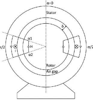
In order to develop a generic model for an 𝑛-phase IM, let’s consider Figure 1.1 which represents an IM with a single winding placed on the inner part of the stator. This winding is supplied with a current 𝑖.

In order to compute the magnetic field, which is produced by the winding, a path that surrounds both its ends is chosen and the Ampere’s law is applied, leading to:

∮ 𝐻⃗⃗ ∙ 𝑑𝑙⃗⃗⃗ = (𝐻1+ 𝐻2) ∙ 𝛿 = [𝐻(𝛼1) + 𝐻(𝛼2)] 𝛿 = 𝑖 (1.1)

By considering that 𝛼1 and 𝛼2 are chosen symmetrical with respect to the conductor, 𝛿 is

constant and we assume that 𝜇𝑓𝑒→ ∞, the magnetic field as a function of the angle 𝛼 is equal

to:

𝐻(𝛼) = 𝑖

(16)

CHAPTER 1:

MULTIPHASE MOTOR MODEL

By considering the geometry of the lines, 𝐻(𝛼) is positive in the mid upper part and negative in the lower one.

From (1.2) it is trivial to compute of the flux density by simply multiplying by 𝜇0.

Hence the flux density 𝐵(𝛼) has the same rectangular behaviour as 𝐻(𝛼) and since it is periodic it can be expressed by means of the Fourier series expansion.

Figure 1.1: Ampere’s law

By considering only the first spatial harmonic: 𝐵𝑠(𝛼) =

4 𝜋

𝜇0

2 𝛿 𝑖 𝑐𝑜𝑠(𝛼) (1.3)

Equations (1.3) can be represented as shown in Figure 1.2.

(17)

If a motor with 𝑝 pole pairs and 𝑧𝑠 turns is considered, the magnetic field first spatial harmonic

can be expressed as:

𝐵𝑠(𝛼) =

2 𝜋

𝜇0 𝑧𝑠

𝛿 𝑖 𝑐𝑜𝑠(𝑝𝛼) (1.4)

Since the turns occupy some space, it is not possible in practice to wind them in a single point, therefore IMs usually have 𝑄 slots where the turns are located and 𝑞𝑠 slots per pole per phase.

In order to account for the phase displacement of 2𝜋 𝑄⁄ , the stator winding factor is introduced: 𝝃𝒔= 𝜉𝑠 𝑒𝑗𝜀= 𝜉𝑠 𝑒

𝑗𝜋(𝑞_𝑄𝑠−1) _(1.5)

Therefore, (1.4) can be rewritten as: 𝐵𝑠(𝛼) = 𝜇0

2 𝑧𝑠 𝑞𝑠 𝜉𝑆

𝜋 𝛿 𝑖 𝑐𝑜𝑠(𝑝𝛼 − 𝜀) (1.6)

Figure 1.3: Example of the effect on B(α) with Q = 20 and qs= 3

Equation (1.6) effect can be seen in Figure 1.3. In any case, it is always possible to move the reference system with the origin in 𝜀, obtaining:

𝐵𝑠(𝛼) = 𝜇0

2 𝑧𝑠 𝑞𝑠 𝜉𝑆

𝜋 𝛿 𝑖 𝑐𝑜𝑠(𝑝𝛼) (1.7)

Now, let’s consider a multiphase IM with 𝑞𝑠= 1. As can it be seen in Figure 1.4, there are n

windings distributed symmetrically around the stator.

The effect of this configuration is of producing a magnetic field for each winding. Since those field lines act radially at the air gap, they can be summed together obtaining:

(18)

CHAPTER 1:

𝐵𝑠(𝛼) = 𝐵𝑠1(𝛼) + 𝐵𝑠2(𝛼) + ⋯ + 𝐵𝑠𝑛(𝛼) = = 𝜇0 2 𝑧𝑠 𝑞𝑠 𝜉𝑆 𝜋 𝛿 [𝑖1cos(𝑝𝛼) + 𝑖2cos (𝑝𝛼 − 2𝜋 𝑛) + ⋯ + 𝑖𝑛cos (𝑝𝛼 − (𝑛 − 1)2𝜋 𝑛 ) ] (1.8) In order to have a more compact form, the complex notation can be used:

𝐵𝑠(𝛼) = 𝜇0 2 𝑧𝑠 𝑞𝑠 𝜉𝑆 𝜋 𝛿 𝑅𝑒 {(∑ 𝑖𝑘+1𝑒 𝑗2𝜋_𝑛𝑘 𝑛−1 𝑘=0 ) 𝑒−𝑗𝑝𝛼} (1.9)

By recalling the definition of the space vector of the stator currents:

𝒊𝑺= 2 𝑛∑ 𝑖𝑘+1𝑒 𝑗2𝜋_𝑛𝑘 𝑛−1 𝑘=0 = 𝐼𝑠 𝑒𝑗𝜓 (1.10)

It is possible to rewrite (1.9) as:

𝐵𝑠(𝛼) = 𝜇0

𝑛 𝑧𝑠 𝑞𝑠 𝜉𝑆

𝜋 𝛿 𝑅𝑒{𝒊𝒔 𝑒

−𝑗𝑝𝛼_} _(1.11)

It is possible to expand (1.11), obtaining something similar to (1.7): 𝐵𝑠(𝛼) = 𝜇0

𝜋 𝛿 𝐼𝑠 cos (𝑝𝛼 − 𝜓) (1.12)

Figure 1.4: n-phase IM with symmetrical distributed phases

By confronting (1.12) with (1.7) it is possible to note that n-windings produce the same effect as a single coil supplied by a current of value equal to 𝑛

2 𝒊𝒔 placed at an angular position equal to

𝜓.

A similar reasoning can be done for the rotor.

(19)

MULTIPHASE MOTOR MODEL 𝐵𝑟(𝛽) = 𝜇0 2 𝑧𝑟 𝑞𝑟 𝜉𝑟 𝜋 𝛿 𝑅𝑒 {( ∑ 𝑖𝑘+1𝑒 𝑗2𝜋_𝑛 𝑟𝑘 𝑛𝑟−1 𝑘=0 ) 𝑒−𝑗𝑝𝛼_} _(1.13)

The space vector of the rotor currents is:

𝒊𝒓′ = 2 𝑛𝑟 ∑ 𝑖𝑟𝑘+1𝑒 𝑗2𝜋_𝑛 𝑟𝑘 𝑛𝑟−1 𝑘=0 (1.14) Therefore (1.13) becomes: 𝐵𝑟(𝛽) = 𝜇0 𝑛𝑟 𝑧𝑟 𝑞𝑟 𝜉𝑟 𝜋 𝛿 𝑅𝑒{𝒊𝒓 ′_𝑒−𝑗𝑝𝛽_} _(1.15)

The effect of the 𝑛𝑟 windings is again the same as a single winding supplied by a current equal

to 𝑛𝑟

2 𝒊𝒓 placed at the phase of 𝒊𝒓.

Now it is of interest the knowledge of the magnetic field at the air gap.

In order to do that, it is necessary to refer both magnetic fields to the same reference system. The chosen reference system is the one integral to the stator, therefore, by looking at Figure 1.5, 𝛽 is:

𝛽 = 𝛼 − 𝜃 (1.16)

So, equation (1.11) remains the same while (1.15) becomes: 𝐵𝑟(𝛼) = 𝜇0

𝑛𝑟 𝑧𝑟 𝑞𝑟 𝜉𝑟

𝜋 𝛿 𝑅𝑒{𝒊𝒓

′_𝑒−𝑗𝑝(𝛼−𝜃)_} _(1.17)

By having both magnetic fields referred to the same reference system, the total air gap field is: 𝐵(𝛼) = 𝐵𝑠(𝛼) + 𝐵𝑟(𝛼) = = 𝜇0 𝑛 𝑧𝑠 𝑞𝑠 𝜉𝑠 𝜋 𝛿 𝑅𝑒{𝒊𝒔 𝑒 −𝑗𝑝𝛼_{} + 𝜇} 0 𝑛𝑟 𝑧𝑟 𝑞𝑟 𝜉𝑟 𝜋 𝛿 𝑅𝑒{𝒊𝒓 ′_𝑒𝑗𝑝𝜃_𝑒−𝑗𝑝𝛼_} (1.18) Since the rotor is normally inaccessible, it is possible to move the rotor current to the stator:

𝜇0 𝑛 𝑧𝑠 𝑞𝑠 𝜉𝑠 𝜋 𝛿 𝒊𝒓= 𝜇0 𝑛𝑟 𝑧𝑟 𝑞𝑟 𝜉𝑟 𝜋 𝛿 𝒊𝒓 ′ 𝒊𝒓= 𝑛𝑟 𝑧𝑟 𝑞𝑟 𝜉𝑟 𝑛 𝑧𝑠 𝑞𝑠 𝜉𝑠 𝒊𝒓′ _(1.19)

Therefore, it is possible to write (1.18) in a more compact form: 𝐵(𝛼) = 𝜇0

𝜋 𝛿 𝑅𝑒{(𝒊𝒔+ 𝒊𝒓 𝑒

(20)

CHAPTER 1:

1.2 Equations

1.2.1 Electrical equations

After having described the magnetic field distribution at the air gap due to stator and rotor windings, it is possible to write the electrical equation of the windings.

By applying Kirchhoff’s voltage law (KVL) to the generic 𝑘-th stator winding: 𝑣𝑠𝑘 = 𝑟𝑠𝑖𝑠𝑘+

𝑑

𝑑𝑡𝜑𝑠𝑘 (1.21)

The generic flux 𝜑𝑠𝑘, can be expressed by the sum of two components:

𝜑𝑠𝑘 = 𝜑𝑠𝑘𝑙+ 𝜑𝑠𝑘𝑚 = 𝑙𝑠𝑖𝑠𝑘+ 𝜑𝑠𝑘𝑚 (1.22)

where subscript 𝑙 indicates the leakage flux due to the flux lines that are close to the same stator windings, while subscript 𝑚 indicates the mutual flux due to the flux lines that cross air gap and rotor.

Figure 1.5: Relation between 𝛼, 𝛽 and 𝜃

By means of (1.22), (1.21) becomes: 𝑣𝑠𝑘 = 𝑟𝑠𝑖𝑠𝑘+ 𝑙𝑠 𝑑 𝑑𝑡𝑖𝑠𝑘+ 𝑑 𝑑𝑡𝜑𝑠𝑘𝑚 (1.23)

The generic mutual flux can be computed integrating the magnetic field considering an hemicylindrical surface placed in the air gap, the diameter 𝐷 of the motor and the axial length 𝑙𝑎𝑥: 𝜑𝑠𝑘𝑚= 𝑝 𝑧𝑠 𝑞𝑠 𝜉𝑠 𝐷 2 𝑙𝑎𝑥 ∫ 𝐵 𝜋 2𝑝+ 2𝜋 𝑛𝑝(𝑘−1) −_2𝑝𝜋+2𝜋_𝑛𝑝(𝑘−1) (𝛼) 𝑑𝛼 =

(21)

MULTIPHASE MOTOR MODEL = 𝑝 𝑧𝑠 𝑞𝑠 𝜉𝑠 𝐷 2 𝑙𝑎𝑥 ∫ 𝜇0 𝑛 𝑧𝑠 𝑞𝑠 𝜉𝑠 𝜋 𝛿 𝑅𝑒{(𝒊𝒔+ 𝒊𝒓 𝑒 𝑗𝑝𝜃_{) 𝑒}−𝑗𝑝𝛼_{} 𝑑𝛼} 𝜋 2𝑝+ 2𝜋 𝑛𝑝(𝑘−1) −_2𝑝𝜋+2𝜋_𝑛𝑝(𝑘−1) = = 𝜇0 𝑛 𝐷 𝑙𝑎𝑥 (𝑧𝑠 𝑞𝑠 𝜉𝑠)2 𝜋 𝛿 𝑝 2 𝑅𝑒 { (𝒊𝒔+ 𝒊𝒓 𝑒𝑗𝑝𝜃) ∫ 𝑒−𝑗𝑝𝛼 𝑑𝛼 𝜋 2𝑝+ 2𝜋 𝑛𝑝(𝑘−1) −_2𝑝𝜋+2𝜋_𝑛𝑝(𝑘−1) } = = 𝜇0 𝑛 𝐷 𝑙𝑎𝑥 (𝑧𝑠 𝑞𝑠 𝜉𝑠)2 𝜋 𝛿 𝑝 2 𝑅𝑒 {(𝒊𝒔+ 𝒊𝒓 𝑒 𝑗𝑝𝜃_{) [}𝑒 −𝑗𝑝𝛼 −𝑗𝑝] −𝜋 2𝑝+ 2𝜋 𝑛𝑝(𝑘−1) 𝜋 2𝑝+ 2𝜋 𝑛𝑝(𝑘−1) } = = 𝜇0 𝑛 𝐷 𝑙𝑎𝑥 (𝑧𝑠 𝑞𝑠 𝜉𝑠)2 𝜋 𝛿 𝑝 2 𝑅𝑒 {(𝒊𝒔+ 𝒊𝒓 𝑒 𝑗𝑝𝜃_)𝑒−𝑗2𝜋_𝑛(𝑘−1) (−2𝑗 −𝑗𝑝)} = = 𝜇0 𝑛 𝐷 𝑙𝑎𝑥 (𝑧𝑠 𝑞𝑠 𝜉𝑠)2 𝜋 𝛿 𝑅𝑒 {(𝒊𝒔+ 𝒊𝒓 𝑒 𝑗𝑝𝜃_)𝑒−𝑗2𝜋_𝑛(𝑘−1)_} (1.24) By recalling the inverse operation of the space vector:

𝑖𝑠𝑘= 𝑅𝑒 {𝒊𝒔𝒌 𝑒−𝑗 2𝜋

𝑛(𝑘−1)_} (1.25)

It is possible to note that the real part extraction in (1.25) is the 𝑘-th stator magnetizing current: 𝑖𝜇𝑠𝑘 = 𝑅𝑒 {𝒊𝝁𝒌 𝑒−𝑗 2𝜋 𝑛(𝑘−1)_{} = 𝑅𝑒 {(𝒊}_𝒔_{+ 𝒊}_𝒓_𝑒𝑗𝑝𝜃_)𝑒−𝑗 2𝜋 𝑛(𝑘−1)_} (1.26) Therefore (1.25) becomes: 𝜑𝑠𝑘𝑚= 𝜇0 𝑛 𝐷 𝑙𝑎𝑥 (𝑧𝑠 𝑞𝑠 𝜉𝑠)2 𝜋 𝛿 𝑖𝜇𝑠𝑘 (1.27)

Since (1.27) express the relation between a flux and a current it is possible to call the terms that multiply 𝑖𝜇𝑘, mutual inductance:

𝐿𝑚= 𝜇0

𝑛 𝐷 𝑙𝑎𝑥 (𝑧𝑠 𝑞𝑠 𝜉𝑠)2

𝜋 𝛿 (1.28)

So, in the end the generic mutual flux is equal to:

𝜑𝑠𝑘𝑚 = 𝐿𝑚𝑖𝜇𝑠𝑘 (1.29) If (1.29) is then substituted in (1.23): 𝑣𝑠𝑘 = 𝑟𝑠𝑖𝑠𝑘+ 𝑙𝑠 𝑑 𝑑𝑡𝑖𝑠𝑘+ 𝐿𝑚 𝑑 𝑑𝑡𝑖𝜇𝑠𝑘 (1.30)

Equation (1.30) can be written for all windings in matrix form, leading to: [𝑣𝑠] = [𝑟𝑠][𝑖𝑠] + [𝑙𝑠] [

𝑑

𝑑𝑡𝑖𝑠] + [𝐿𝑚] [ 𝑑

𝑑𝑡𝑖𝜇𝑠] (1.31)

In order to simplify the model, an equivalent machine is considered.

In order to do so, it is necessary to transform the real machine model into the equivalent one. For this purpose, the transformation matrix [𝑇𝑛] is introduced [3], with 𝜃 = 2𝜋 𝑛⁄ :

(22)

CHAPTER 1:

[𝑇𝑛] =

2 𝑛

[

1 cos(𝜃) cos(2𝜃) cos(3𝜃) ⋯ cos(3𝜃) cos(2𝜃) cos(𝜃)

0 sin(𝜃) sin(2𝜃) sin(3𝜃) ⋯ − sin(3𝜃) −sin(2𝜃) −sin(𝜃)

1 cos(2𝜃) cos(4𝜃) cos(6𝜃) ⋯ cos(6𝜃) cos(4𝜃) cos(2𝜃)

0 sin(2𝜃) sin(4𝜃) sin(6𝜃) ⋯ −sin(6𝜃) −sin(4𝜃) −sin(2𝜃)

1 cos(3𝜃) cos(6𝜃) cos(9𝜃) ⋯ cos(9𝜃) cos(6𝜃) cos(3𝜃)

0 sin(3𝜃) sin(6𝜃) sin(9𝜃) ⋯ −sin(9𝜃) − sin(6𝜃) − sin(3𝜃)

⋯ ⋯ ⋯ ⋯ ⋯ ⋯ ⋯ ⋯ 1 cos (𝑛 − 2 2 𝜃) cos (2 𝑛 − 2 2 𝜃) cos (3 𝑛 − 2 2 𝜃) ⋯ cos (3 𝑛 − 2 2 𝜃) cos (2 𝑛 − 2 2 𝜃) cos ( 𝑛 − 2 2 𝜃) 0 sin (𝑛 − 2 2 𝜃) sin (2 𝑛 − 2 2 𝜃) sin (3 𝑛 − 2 2 𝜃) ⋯ − sin (3 𝑛 − 2 2 𝜃) −sin (2 𝑛 − 2 2 𝜃) −sin ( 𝑛 − 2 2 𝜃) 1 2 ⁄ 1⁄₂ 1⁄₂ 1⁄₂ ⋯ 1⁄₂ 1⁄₂ 1⁄₂ 1 2 ⁄ _{− 1 2}⁄ 1⁄₂ _{− 1 2}⁄ ⋯ _{− 1 2}⁄ 1⁄₂ _{− 1 2}⁄ _] (1.32)

If 𝑛 is odd the result of (𝑛−2)

2 must be rounded to the next integer.

If (1.32) is applied to an appropriate vector, a new vector with same dimensions as the original one will be obtained. It is also possible to apply the inverse of [𝑇𝑛] in order to obtain the original

vector starting from a transformed one. By applying (1.32) to (1.31): [𝑇𝑛][𝑣𝑠] = [𝑇𝑛][𝑟𝑠][𝑖𝑠] + [𝑇𝑛][𝑙𝑠] [ 𝑑 𝑑𝑡𝑖𝑠] + [𝑇𝑛][𝐿𝑚] [ 𝑑 𝑑𝑡𝑖𝜇𝑠] [𝑣𝑠𝑡𝑟] = [𝑇𝑛][𝑟𝑠][𝑇𝑛]−1[𝑖𝑠𝑡𝑟] + [𝑇𝑛][𝑙𝑠][𝑇𝑛]−1[ 𝑑 𝑑𝑡𝑖𝑠𝑡𝑟] + [𝑇𝑛][𝐿𝑚][𝑇𝑛] −1_[𝑑 𝑑𝑡𝑖𝜇𝑠𝑡𝑟] [𝑣𝑠𝑡𝑟] = [𝑟𝑠][𝑖𝑠𝑡𝑟] + [𝑙𝑠] [ 𝑑 𝑑𝑡𝑖𝑠𝑡𝑟] + [𝐿𝑚] [ 𝑑 𝑑𝑡𝑖𝜇𝑠𝑡𝑟] (1.33)

The transformed stator equations are obtained.

Since the real model had 𝑛 independent variables, the equivalent one must have the same number of them, but only the first two rows actually produce torque and flux, the last two are zero sequence component while the remaining are equations decoupled from the others, that cause only joule losses and therefore, should be minimized for the best performance during normal duty but can be controlled during fault operations in order to allow the machine to continue working. This characteristic is what distinguish multiphase motors from simple 3-phase machines.

Concerning the rotor, the same approach used for the stator can be followed. The KVL to the 𝑘-th rotor winding lead to:

𝑣𝑟𝑘′ = 𝑟𝑟′𝑖𝑟𝑘′ + 𝑙𝑟′

𝑑 𝑑𝑡𝑖𝑟𝑘

′ ₊ 𝑑

𝑑𝑡𝜑𝑟𝑘𝑚 (1.34)

Therefore, there’s the need to compute 𝜑𝑟𝑘𝑚:

𝜑𝑟𝑘𝑚= 𝑝 𝑧𝑟 𝑞𝑟 𝜉𝑟 𝐷 2 𝑙𝑎𝑥 ∫ 𝐵 𝜋 2𝑝+ 2𝜋 𝑛𝑟𝑝(𝑘−1) −𝜋 2𝑝+ 2𝜋 𝑛𝑟𝑝(𝑘−1) (𝛽) 𝑑𝛽 =

(23)

MULTIPHASE MOTOR MODEL = 𝑝 𝑧𝑟 𝑞𝑟 𝜉𝑟 𝐷 2 𝑙𝑎𝑥 ∫ 𝜇0 𝑛 𝑧𝑠 𝑞𝑠 𝜉𝑠 𝜋 𝛿 𝑅𝑒{(𝒊𝒔𝑒 −𝑗𝑝𝜃_{+ 𝒊} 𝒓 ) 𝑒−𝑗𝑝𝛽} 𝑑𝛽 𝜋 2𝑝+ 2𝜋 𝑛𝑟𝑝(𝑘−1) −_2𝑝𝜋+_𝑛2𝜋 𝑟𝑝(𝑘−1) = = 𝜇0 𝑛 𝐷 𝑙𝑎𝑥 𝑧𝑟 𝑞𝑟 𝜉𝑟 𝑧𝑠 𝑞𝑠 𝜉𝑠 𝜋 𝛿 𝑝 2 𝑅𝑒 { (𝒊𝒔𝑒−𝑗𝑝𝜃+ 𝒊𝒓 ) ∫ 𝑒−𝑗𝑝𝛽 𝑑𝛽 𝜋 2𝑝+ 2𝜋 𝑛_𝑟𝑝(𝑘−1) −𝜋 2𝑝+ 2𝜋 𝑛𝑟𝑝(𝑘−1) } = = 𝜇0 𝑛 𝐷 𝑙𝑎𝑥 𝑧𝑠 𝑞𝑠 𝜉𝑠 𝜋 𝛿 𝑧𝑟 𝑞𝑟 𝜉𝑟 𝑅𝑒 {(𝒊𝒔𝑒 −𝑗𝑝𝜃_{+ 𝒊} 𝒓 )𝑒 −𝑗2𝜋 𝑛𝑟(𝑘−1)} (1.35) By introducing the rotor magnetizing current:

𝑖𝜇𝑟𝑘= 𝑅𝑒 {(𝒊𝒔𝑒−𝑗𝑝𝜃+ 𝒊𝒓 )𝑒 −𝑗2𝜋_𝑛

𝑟(𝑘−1)} (1.36)

If (1.28) and (1.36) are considered, equation (1.35) can be written as: 𝜑𝑟𝑘𝑚=

𝑧𝑟 𝑞𝑟 𝜉𝑟

𝑧𝑠 𝑞𝑠 𝜉𝑠

𝐿𝑚𝑖𝜇𝑟𝑘 (1.37)

By using (1.37) into (1.34) and by considering that usually the rotor windings are closed in short circuit: 0 = 𝑟𝑟′𝑖𝑟𝑘′ + 𝑙𝑟′ 𝑑 𝑑𝑡𝑖𝑟𝑘 ′ ₊𝑧𝑟 𝑞𝑟 𝜉𝑟 𝑧𝑠 𝑞𝑠 𝜉𝑠 𝐿𝑚 𝑑 𝑑𝑡𝑖𝜇𝑟𝑘 (1.38)

By considering (1.19), solved for 𝒊𝒓′, into (1.38):

0 = 𝑛 𝑧𝑠 𝑞𝑠 𝜉𝑠 𝑛𝑟 𝑧𝑟 𝑞𝑟 𝜉𝑟 𝑟𝑟′𝑖𝑟𝑘+ 𝑛 𝑧𝑠 𝑞𝑠 𝜉𝑠 𝑛𝑟 𝑧𝑟 𝑞𝑟 𝜉𝑟 𝑙𝑟′ 𝑑 𝑑𝑡𝑖𝑟𝑘+ 𝑧𝑟 𝑞𝑟 𝜉𝑟 𝑧𝑠 𝑞𝑠 𝜉𝑠 𝐿𝑚 𝑑 𝑑𝑡𝑖𝜇𝑟𝑘 0 = 𝑛 (𝑧𝑠 𝑞𝑠 𝜉𝑠) 2 𝑛𝑟 (𝑧𝑟 𝑞𝑟 𝜉𝑟)2 𝑟𝑟′𝑖𝑟𝑘+ 𝑛 (𝑧𝑠 𝑞𝑠 𝜉𝑠)2 𝑛𝑟 (𝑧𝑟 𝑞𝑟 𝜉𝑟)2 𝑙𝑟′ 𝑑 𝑑𝑡𝑖𝑟𝑘+ 𝐿𝑚 𝑑 𝑑𝑡𝑖𝜇𝑟𝑘 (1.39) By defining: 𝑟𝑟= 𝑛 (𝑧𝑠 𝑞𝑠 𝜉𝑠)2 𝑛𝑟 (𝑧𝑟 𝑞𝑟 𝜉𝑟)2 𝑟𝑟′ (1.40) 𝑙𝑟= 𝑛 (𝑧𝑠 𝑞𝑠 𝜉𝑠)2 𝑛𝑟 (𝑧𝑟 𝑞𝑟 𝜉𝑟)2 𝑙𝑟′ (1.41)

It is possible to write the KVL for all the rotor windings in the matrix form: [𝑣𝑟] = [𝑟𝑟][𝑖𝑟] + [𝑙𝑟] [

𝑑

𝑑𝑡𝑖𝑟] + [𝐿𝑚] [ 𝑑

𝑑𝑡𝑖𝜇𝑟] (1.42)

Now if (1.32) is applied to both sides of (1.42): [𝑇𝑛][𝑣𝑟] = [𝑇𝑛][𝑟𝑟][𝑖𝑟] + [𝑇𝑛][𝑙𝑟] [ 𝑑 𝑑𝑡𝑖𝑟] + [𝑇𝑛][𝐿𝑚] [ 𝑑 𝑑𝑡𝑖𝜇𝑟] [𝑣𝑟𝑡𝑟] = [𝑇𝑛][𝑟𝑟][𝑇𝑛]−1[𝑖𝑠𝑡𝑟] + [𝑇𝑛][𝑙𝑠][𝑇𝑛]−1[ 𝑑 𝑑𝑡𝑖𝑠𝑡𝑟] + [𝑇𝑛][𝐿𝑚][𝑇𝑛] −1_[𝑑 𝑑𝑡𝑖𝜇𝑠𝑡𝑟] [𝑣𝑟𝑡𝑟] = [𝑟𝑟][𝑖𝑟𝑡𝑟] + [𝑙𝑟] [ 𝑑 𝑑𝑡𝑖𝑟𝑡𝑟] + [𝐿𝑚] [ 𝑑 𝑑𝑡𝑖𝜇𝑟𝑡𝑟] (1.43)

(24)

CHAPTER 1:

The transformed rotor equations are obtained, completing the electrical model of a multiphase motor.

In order to complete the electrical equations, the electromechanical torque that the motor can develop is needed.

The electromagnetic torque 𝑇 that the motor can develop, is computed considering a uniform current distribution at the air gap, which leads to a sinusoidal distribution of the magnetic field. In order to compute the torque, the rotor current distribution is considered. Same reasoning can be done considering the stator current distribution with the only difference of a minus sign. By considering this, the Ampere’s law for the rotor can be written as:

[𝐻𝑟(𝛼1) − 𝐻𝑟(𝛼2)]𝛿 = ∫ 𝛤𝑟(𝛼) 𝑑𝛼 𝛼2 𝛼₁ lim 𝛼2→𝛼1 [𝐻_𝑟(𝛼₁) − 𝐻_𝑟(𝛼₂)]𝛿 = −𝑑𝐻_𝑟(𝛼)𝛿 = 𝛤_𝑟(𝛼) 𝑑𝛼 _(1.44) Therefore, from (1.44) it is possible to compute 𝛤𝑟(𝛼):

𝛤𝑟(𝛼) = −

𝑑

𝑑𝛼[𝐻𝑟(𝛼) 𝛿] (1.45)

By substituting only the rotor component of (1.20) into (1.45): 𝛤𝑟(𝛼) = − 𝑑 𝑑𝛼[𝐻𝑟(𝛼) 𝛿] = − 𝑑 𝑑𝛼[ 𝐵𝑟(𝛼) 𝜇0 𝛿] = = − 𝑑 𝑑𝛼[ 𝑛 𝑧𝑠 𝑞𝑠 𝜉𝑆 𝜋 𝑅𝑒{𝒊𝒓 𝑒 𝑗𝑝𝜃_𝑒−𝑗𝑝𝛼_{}] =} = −𝑛 𝑧𝑠 𝑞𝑠 𝜉𝑆 𝜋 𝑅𝑒 {𝒊𝒓 𝑒 𝑗𝑝𝜃 𝑑 𝑑𝛼 [𝑒 −𝑗𝑝𝛼_{]} =} = −𝑛 𝑧𝑠 𝑞𝑠 𝜉𝑆 𝜋 𝑅𝑒{−𝑗𝑝 𝒊𝒓 𝑒 𝑗𝑝𝜃_𝑒−𝑗𝑝𝛼_{} =} = −𝑛 𝑧𝑠 𝑞𝑠 𝜉𝑆 𝜋 𝑝 𝐼𝑚{𝒊𝒓 𝑒 𝑗𝑝𝜃_𝑒−𝑗𝑝𝛼_} (1.46) The electromagnetic torque can be computed by integrating the elemental Lorentz’s force over the rotor: 𝑇 =𝐷 2𝑙𝑎𝑥 𝑝 ∫ 𝐵(𝛼)𝛤𝑟(𝛼) 𝑑𝛼 2𝜋 𝑝 0 = = −𝑛 2 𝑝2 𝜋 [𝜇0 𝑛 𝐷 𝑙𝑎𝑥 (𝑧𝑠 𝑞𝑠 𝜉𝑠)2 𝜋 𝛿 ] ∫ 𝑅𝑒{(𝒊𝒔+ 𝒊𝒓 𝑒 𝑗𝑝𝜃_{) 𝑒}−𝑗𝑝𝛼_{} 𝐼𝑚{𝒊} 𝒓 𝑒𝑗𝑝𝜃𝑒−𝑗𝑝𝛼} 𝑑𝛼 2𝜋 𝑝 0 = −𝑛 2 𝑝2 𝜋 𝐿𝑚∫ 𝑅𝑒{(𝒊𝒔+ 𝒊𝒓 𝑒 𝑗𝑝𝜃_{) 𝑒}−𝑗𝑝𝛼_{} 𝐼𝑚{𝒊} 𝒓 𝑒𝑗𝑝𝜃𝑒−𝑗𝑝𝛼} 𝑑𝛼 2𝜋 𝑝 0 (1.47)

(25)

𝒊𝒔= 𝑖𝑠𝑟+ 𝑗𝑖𝑠𝑖

𝒊𝒓 𝑒𝑗𝑝𝜃 = 𝑖𝑟𝑟+ 𝑗𝑖𝑟𝑖 (1.48)

If (1.48) is used into (1.47) and the Euler’s equation for 𝑒−𝑗𝑝𝛼_{is considered:}

𝑇 = −𝑛 2

𝑝2

𝜋 𝐿𝑚∫ [𝑖𝑠𝑟cos(𝑝𝛼) + 𝑖𝑠𝑖sin(𝑝𝛼) + 𝑖𝑟𝑟cos(𝑝𝛼) + 𝑖𝑟𝑖sin(𝑝𝛼)]

2𝜋 𝑝 0 ∙ ∙ [−𝑖𝑟𝑟sin(𝑝𝛼) + 𝑖𝑟𝑖cos(𝑝𝛼)] 𝑑𝛼 (1.49)

It is worth recalling that:

∫ cos2_{(𝑝𝛼) 𝑑𝛼} 2𝜋 𝑝 0 = ∫ sin2_{(𝑝𝛼) 𝑑𝛼} 2𝜋 𝑝 0 =𝜋 𝑝 (1.50) ∫ cos(𝑝𝛼) sin(𝑝𝛼) 𝑑𝛼 2𝜋 𝑝 0 = 0 (1.51) By using (1.50) and (1.51) in (1.49): 𝑇 = −𝑛 2 𝑝2 𝜋 𝐿𝑚[ 𝜋 𝑝(𝑖𝑠𝑟𝑖𝑟𝑖− 𝑖𝑠𝑖𝑖𝑟𝑟+ 𝑖𝑟𝑟𝑖𝑟𝑖− 𝑖𝑟𝑟𝑖𝑟𝑖)] = = −𝑛 2 𝑝 𝐿𝑚(𝑖𝑠𝑟𝑖𝑟𝑖− 𝑖𝑠𝑖𝑖𝑟𝑟) = =𝑛 2 𝑝 𝐿𝑚 𝐼𝑚{𝒊𝒔 (𝒊𝒓𝑒 𝑗𝑝𝜃₎∗_} (1.52)

(26)

CHAPTER 1:

1.2.2 Mechanical equations

In order to complete the model also the mechanical equations are needed.

The motor, as said in the previous chapter, can develop a torque. This torque is applied to other mechanical devices which could apply a load torque 𝑇𝐿. In general, motors and mechanical

devices have some inertia which summed together gives the total inertia 𝐽 of the system. At last the rotation of the motor can be slowed by air friction which is accounted by the coefficient 𝐵. In order to account all of this, it can be written:

𝑇 − 𝑇𝐿= 𝐽

𝑑

𝑑𝑡𝜔𝑟+ 𝐵𝜔𝑟 (1.53)

In (1.53) appears the rotor mechanical speed 𝜔𝑟, which can be measured.

From its knowledge, it is possible to compute the rotor position as:

𝜃 = 𝜃0+ ∫ 𝜔𝑟𝑑𝑡 𝑡

0 (1.54)

Where 𝜃0 is the rotor initial position.

1.2.3 Complete model

After computing electrical and mechanical equations, the complete model of a generic multiphase motor, becomes:

{ [𝑣𝑠𝑡𝑟] = [𝑟𝑠][𝑖𝑠𝑡𝑟] + [𝑙𝑠] [ 𝑑 𝑑𝑡𝑖𝑠𝑡𝑟] + [𝐿𝑚] [ 𝑑 𝑑𝑡𝑖𝜇𝑠𝑡𝑟] [𝑣_𝑟𝑡𝑟] = [𝑟_𝑟][𝑖_𝑟𝑡𝑟] + [𝑙_𝑟] [𝑑 𝑑𝑡𝑖𝑟𝑡𝑟] + [𝐿𝑚] [ 𝑑 𝑑𝑡𝑖𝜇𝑟𝑡𝑟] 𝑇 =𝑛 2 𝑝 𝐿𝑚 𝐼𝑚{𝒊𝒔 𝒊𝒓 𝒔 ∗_} 𝑇 − 𝑇𝐿= 𝐽 𝑑 𝑑𝑡𝜔𝑟+ 𝐵𝜔𝑟 𝜃 = 𝜃0+ ∫ 𝜔𝑟𝑑𝑡 𝑡 0 (1.55)

(27)

1.3 Case study: 5-Phase IM

The results obtained can be applied in order to compute the model of a 5-phase IM. The transformation matrix (1.32) for a 5-phase machine, becomes:

[𝑇5] =

2 5 [

1 cos(𝜃) cos(2𝜃) cos(3𝜃) cos(4𝜃) 0 sin(𝜃) sin(𝜃) sin(𝜃) sin(𝜃) 1 cos(2𝜃) cos(4𝜃) cos(𝜃) cos(3𝜃) 0 sin(2𝜃) sin(4𝜃) sin(𝜃) sin(3𝜃) 1

2

⁄ 1⁄₂ 1⁄₂ 1⁄₂ 1⁄₂ _]

(1.56)

With 𝜃 = 2𝜋⁄ . ₅

The generic stator and rotor equations can be written in matrix form:

{ [𝑣𝑠12345] = [𝑟𝑠][𝑖𝑠12345] + [𝑙𝑠] [ 𝑑 𝑑𝑡𝑖𝑠12345] + [𝐿𝑚] [ 𝑑 𝑑𝑡𝑖𝜇𝑠12345] [𝑣𝑟12…𝑛_𝑟] = [𝑟𝑟][𝑖𝑟12…𝑛_𝑟] + [𝑙𝑟] [ 𝑑 𝑑𝑡𝑖𝑟12…𝑛𝑟] + [𝐿𝑚] [ 𝑑 𝑑𝑡𝑖𝜇𝑟12…𝑛𝑟] (1.57)

If (1.56) is applied to the stator equation of (1.57): [𝑣𝑠𝛼𝛽𝑥𝑦𝑧] = [𝑟𝑠][𝑖𝑠𝛼𝛽𝑥𝑦𝑧] + [𝑙𝑠] [ 𝑑 𝑑𝑡𝑖𝑠𝛼𝛽𝑥𝑦𝑧] + [𝐿𝑚] [ 𝑑 𝑑𝑡𝑖𝜇𝑠𝛼𝛽𝑥𝑦𝑧] (1.58)

Since the neutral point of the machine is inaccessible, the zero component can be disregarded. If a transformation matrix is applied to the rotor equations of (1.57), it is observed that the only components with excitation terms are the 𝛼𝛽 ones [4] [5], hence:

[𝑣𝑟𝛼𝛽] = [𝑟𝑟][𝑖𝑟𝛼𝛽] + [𝑙𝑟] [

𝑑

𝑑𝑡𝑖𝑟𝛼𝛽] + [𝐿𝑚] [ 𝑑

𝑑𝑡𝑖𝜇𝑟𝛼𝛽] (1.59)

Therefore, the model can be expressed in the following way by exploiting the space vector notation: { 𝒗𝒔= 𝑟𝑠𝒊𝒔+ (𝑙𝑠+ 𝐿𝑚) 𝑑 𝑑𝑡𝒊𝒔+ 𝐿𝑚 𝑑 𝑑𝑡(𝒊𝒓𝑒 𝑗𝑝𝜃₎ 𝒗𝒔𝒙𝒚= 𝑟𝑠𝒊𝒔𝒙𝒚+ 𝑙𝑠 𝑑 𝑑𝑡𝒊𝒔𝒙𝒚 0 = 𝑟𝑟𝒊𝒓+ (𝑙𝑟+ 𝐿𝑚) 𝑑 𝑑𝑡𝒊𝒓+ 𝐿𝑚 𝑑 𝑑𝑡(𝒊𝒔𝑒 −𝑗𝑝𝜃₎ 𝑇 =5 2𝑝𝐿𝑚𝐼𝑚{𝒊𝒔(𝒊𝒓𝑒 𝑗𝑝𝜃₎∗_} 𝑇 − 𝑇𝐿= 𝐽 𝑑 𝑑𝑡𝜔𝑟+ 𝐵𝜔𝑟 𝜃 = ∫ 𝜔𝑟𝑑𝑡 𝑡 0 + 𝜃0 (1.60)

It is possible to define some quantities:

𝐿𝑠= 𝑙𝑠+ 𝐿𝑚 (1.61)

𝐿𝑟= 𝑙𝑟+ 𝐿𝑚 (1.62)

(28)

CHAPTER 1:

𝝋𝒔= 𝐿𝑠𝒊𝒔+ 𝐿𝑚𝒊𝒓𝒔 (1.64) 𝝋𝒓= 𝐿𝑚𝒊𝒔+ 𝐿𝑟𝒊𝒓𝒔 (1.65) 𝑑 𝑑𝑡(𝒙𝑒 ±𝑗𝑝𝜃_{) = 𝑒}±𝑗𝑝𝜃 𝑑 𝑑𝑡𝒙 ± 𝑗𝑝𝜔𝑟𝒙𝑒 ±𝑗𝑝𝜃 (1.66)

By considering (1.61), (1.62), (1.63), (1.64), (1.66) and by multiplying the rotor equation by 𝑒𝑗𝑝𝜃_,

it is possible to rewrite (1.60) as:

{ 𝒗𝒔= 𝑟𝑠𝒊𝒔+ 𝐿𝑠 𝑑 𝑑𝑡𝒊𝒔+ 𝐿𝑚 𝑑 𝑑𝑡𝒊𝒓 𝒔 𝒗𝒔𝒙𝒚= 𝑟𝑠𝒊𝒔𝒙𝒚+ 𝑙𝑠 𝑑 𝑑𝑡𝒊𝒔𝒙𝒚 𝟎 = 𝑟𝑟𝒊𝒓𝒔+ 𝐿𝑟 𝑑 𝑑𝑡𝒊𝒓 𝒔_{+ 𝐿} 𝑚 𝑑 𝑑𝑡𝒊𝒔− 𝑗𝑝𝜔𝑟(𝐿𝑚𝒊𝒔+ 𝐿𝑟𝒊𝒓 𝒔₎ 𝑇 =5 2𝑝𝐿𝑚𝐼𝑚{𝒊𝒔𝒊𝒓 𝒔 ∗_} 𝑇 − 𝑇𝐿= 𝐽 𝑑 𝑑𝑡𝜔𝑟+ 𝐵𝜔𝑟 𝜃 = ∫ 𝜔𝑟𝑑𝑡 𝑡 0 + 𝜃0 (1.67)

Obtaining the 9th_{order model of a 5-phase IM.}

1.3.1 Model in term of fluxes

It is possible to model a 5-phase IM in term of fluxes in order to create a Matlab/Simulink model.

From (1.65) it is possible to express 𝒊𝒓𝒔 as:

𝒊𝒓𝒔= 𝝋𝒓 𝐿𝑟 −𝐿𝑚 𝐿𝑟 𝒊𝒔 (1.68)

By substituting (1.68) in (1.64), it is possible to solve for 𝒊𝒔 obtaining:

𝒊𝒔= 𝝋𝒔 (𝐿𝑠−𝐿𝑚 2 𝐿𝑟) − 𝐿𝑚 𝐿𝑟(𝐿𝑠−𝐿𝑚 2 𝐿𝑟) 𝝋𝒓 (1.69)

By projecting (1.69) on the 𝛼𝛽 axis: 𝑖𝑠𝛼= 𝜑𝑠𝛼 (𝐿𝑠− 𝐿2𝑚 𝐿𝑟) − 𝐿𝑚 𝐿𝑟(𝐿𝑠− 𝐿2𝑚 𝐿𝑟) 𝜑𝑟𝛼 𝑖𝑠𝛽= 𝜑𝑠𝛽 (𝐿𝑠− 𝐿2𝑚 𝐿𝑟) − 𝐿𝑚 𝐿𝑟(𝐿𝑠− 𝐿2𝑚 𝐿𝑟) 𝜑𝑟𝛽 (1.70)

From the machine model (1.67) it can be observed that: 𝒗𝒔 = 𝑟𝑠𝒊𝒔+

𝑑 𝑑𝑡𝝋𝒔

(29)

Therefore, it is possible to solve (1.71) for 𝑑

𝑑𝑡𝜑𝑠𝛼 and 𝑑 𝑑𝑡𝜑𝑠𝛽, obtaining: 𝑑 𝑑𝑡𝜑𝑠𝛼= 𝑣𝑠𝛼− 𝑟𝑠𝑖𝑠𝛼 𝑑 𝑑𝑡𝜑𝑠𝛽 = 𝑣𝑠𝛽− 𝑟𝑠𝑖𝑠𝛽 (1.72) If (1.70) is substituted in (1.72): 𝑑 𝑑𝑡𝜑𝑠𝛼 = 𝑣𝑠𝛼− 𝑟𝑠 (𝐿𝑠−𝐿𝑚 2 𝐿𝑟) 𝜑𝑠𝛼+ 𝑟𝑠𝐿𝑚 𝐿𝑟(𝐿𝑠−𝐿𝑚 2 𝐿𝑟) 𝜑𝑟𝛼 𝑑 𝑑𝑡𝜑𝑠𝛽= 𝑣𝑠𝛽− 𝑟𝑠 (𝐿𝑠− 𝐿2𝑚 𝐿𝑟) 𝜑𝑠𝛽+ 𝑟𝑠𝐿𝑚 𝐿𝑟(𝐿𝑠− 𝐿2𝑚 𝐿𝑟) 𝜑𝑟𝛽 (1.73)

A similar reasoning can be followed for the rotor fluxes.

From (1.64) 𝒊𝒔 is obtained then it is used in (1.65) to obtain 𝒊𝒓𝒔, which decomposed onto 𝛼𝛽 axis

gives: 𝑖𝑟𝛼= 𝜑𝑟𝛼 (𝐿𝑟−𝐿𝑚 2 𝐿𝑠) − 𝐿𝑚 𝐿𝑠(𝐿𝑟−𝐿𝑚 2 𝐿𝑠) 𝜑𝑠𝛼 𝑖𝑟𝛽= 𝜑𝑟𝛽 (𝐿𝑟−𝐿𝑚 2 𝐿𝑠) − 𝐿𝑚 𝐿𝑠(𝐿𝑟−𝐿𝑚 2 𝐿𝑠) 𝜑𝑠𝛽 (1.74)

The voltage equation for the rotor can be obtained also in this case from the machine model (1.67):

𝟎 = 𝑟𝑟𝒊𝒔+

𝑑

𝑑𝑡𝝋𝒓− 𝑗𝑝𝜔𝑟𝝋𝒓

(1.75)

From (1.75) it is possible to solve for 𝑑

𝑑𝑡𝜑𝑟𝛼 and 𝑑 𝑑𝑡𝜑𝑟𝛽 and by substituting (1.74): 𝑑 𝑑𝑡𝜑𝑟𝛼= − 𝑟𝑟 (𝐿𝑟− 𝐿2𝑚 𝐿𝑠) 𝜑𝑟𝛼+ 𝑟𝑟𝐿𝑚 𝐿𝑠(𝐿𝑟− 𝐿𝑚2 𝐿𝑠) 𝜑𝑠𝛼− 𝑝𝜔𝑟𝜑𝑟𝛽 𝑑 𝑑𝑡𝜑𝑟𝛽= − 𝑟𝑟 (𝐿𝑟−𝐿𝑚 2 𝐿𝑠) 𝜑𝑟𝛽+ 𝑟𝑟𝐿𝑚 𝐿𝑠(𝐿𝑟−𝐿𝑚 2 𝐿𝑠) 𝜑𝑠𝛽+ 𝑝𝜔𝑟𝜑𝑟𝛼 (1.76)

When the machine is supplied, the only unknowns are the fluxes. Those can be computed integrating (1.73) and (1.76). After computing the fluxes, it is possible to use them in (1.70) and (1.74) to compute the stator and rotor 𝛼𝛽 currents.

In order to compute the 𝑥𝑦 components of the stator current, the machine model (1.67) can be used: 𝑑 𝑑𝑡𝑖𝑠𝑥= 1 𝑙𝑠 [𝑣𝑥− 𝑟𝑠𝑖𝑠𝑥] 𝑑 𝑑𝑡𝑖𝑠𝑦= 1 𝑙𝑠 [𝑣𝑦− 𝑟𝑠𝑖𝑠𝑦] (1.77)

(30)

CHAPTER 2:

CONTROL MODEL

In this chapter a brief introduction on the different control techniques is given. Then a rotor field-oriented control (RFOC) model for a n-phase IM, its scheme and tuning are presented and a 𝑛-phase voltage source inverter (VSI) model is computed.

2.1 Controls

In control theory there are two major classes: 1. Scalar controls

2. Vector controls

The first one is a control technique that is aimed on controlling the steady state behaviour of a machine. It doesn’t matter how it reaches it as long as the steady state value is obtained. The second one, is a control technique, of which the RFOC belongs, that is aimed on controlling dynamically the machines. Therefore, it is possible to control them instant by instant.

For both control techniques, PI regulators are used in order to control the key quantities.

2.2 PI regulators

Proportional-integral (PI) controllers, are a family of control mechanisms that employ feedback. These types of controllers are used to control that a certain quantity reaches a desired value. This is achieved by minimizing an error, which is obtained by subtracting the actual signal to the reference signal.

The following parameters computation is valid for all linear systems that can be expressed as: 𝐴 𝑑

𝑑𝑡𝑦 + 𝐵𝑦 = 𝐶 (2.1)

Where 𝑦 is the parameter under control, 𝐴 and 𝐵 are system parameters and 𝐶 is a control quantity.

(31)

CONTROL MODEL

A scheme for a PI controller can be seen in Figure 2.1.

Figure 2.1: PI regulator scheme

Where 𝑘𝑝 is the proportional coefficient and 𝑘𝑖 is the integral coefficient.

In order to define how to find 𝑘𝑝 and 𝑘𝑖 as a function of the parameters 𝐴 and 𝐵, let’s write the

closed loop transfer function:

𝑊(𝑠) = (𝑘𝑝+ 𝑘𝑖 𝑠) ( 1 𝑠𝐴 + 𝐵) 1 + (𝑘𝑝+𝑘_𝑠𝑖) (_{𝑠𝐴 + 𝐵}1 ) = = (𝑠𝑘𝑝+ 𝑘𝑖) 𝑠(𝑠𝐴 + 𝐵) + 𝑠𝑘𝑝+ 𝑘𝑖 (2.2) If in (2.2) 𝑠 = 𝑗𝜔 is used: 𝑊(𝑗𝜔) = (𝑗𝜔𝑘𝑝+ 𝑘𝑖) 𝑗𝜔(𝑗𝜔𝐴 + 𝐵) + 𝑗𝜔𝑘𝑝+ 𝑘𝑖 = = 𝑗𝜔𝑘𝑝+ 𝑘𝑖 −𝜔2_{𝐴 + 𝑗𝜔(𝐵 + 𝑘} 𝑝) + 𝑘𝑖 (2.3)

The cut-off frequency is the value at which the magnitude of 𝑊(𝑠) is −3𝑑𝐵: |𝑊(𝑗𝜔𝑐)|2= 𝜔𝑐2𝑘𝑝2+ 𝑘𝑖2 (𝑘𝑖− 𝜔𝑐2𝐴)2+ (𝜔𝑐𝐵 + 𝜔𝑐𝑘𝑝) 2= 1 2 _(2.4)

Therefore, by solving for 𝑘𝑖:

𝑘𝑖= −𝜔𝑐2𝐴 ± 𝜔𝑐√2𝜔𝑐2𝐴2− 𝑘𝑝2+ 2𝐵𝑘𝑝+ 𝐵2 _(2.5)

The only possible solution is a positive-real one, therefore:

{𝑘𝑖= −𝜔𝑐 2_{𝐴 ± 𝜔} 𝑐√2𝜔𝑐2𝐴2− 𝑘𝑝2+ 2𝐵𝑘𝑝+ 𝐵2> 0 2𝜔𝑐2𝐴2− 𝑘𝑝2+ 2𝐵𝑘𝑝+ 𝐵2> 0 (2.6) By solving for 𝑘𝑝: 𝑘𝑝= 𝑥 (𝐵 + √2𝐵2+ 𝜔𝑐2𝐴2) (2.7) Where 𝑥 ∈ (0, 1].

(32)

CHAPTER 2: CONTROL MODEL

Therefore, both coefficients are defined as:

{

𝑘𝑝= 𝑥 (𝐵 + √2𝐵2+ 𝜔𝑐2𝐴2)

𝑘𝑖= −𝜔𝑐2𝐴 ± 𝜔𝑐√2𝜔𝑐2𝐴2− 𝑘𝑝2+ 2𝐵𝑘𝑝+ 𝐵2 _(2.8)

The maximum cut-off frequency , of the following controls, is one decade less than the switching frequency of the VSI.

2.3 RFOC

As previously said, this kind of control technique is able to monitor the machine behaviour instant by instant.

For any 𝑛-phase IM it is possible to write stator and rotor equations equal to the ones of (1.69):

{ 𝒗𝒔 = 𝑟𝑠𝒊𝒔+ 𝐿𝑠 𝑑 𝑑𝑡𝒊𝒔+ 𝐿𝑚 𝑑 𝑑𝑡𝒊𝒓 𝒔 𝟎 = 𝑟𝑟𝒊𝒓𝒔+ 𝐿𝑟 𝑑 𝑑𝑡𝒊𝒓 𝒔_{+ 𝐿} 𝑚 𝑑 𝑑𝑡𝒊𝒔− 𝑗𝑝𝜔𝑟(𝐿𝑚𝒊𝒔+ 𝐿𝑟𝒊𝒓 𝒔₎ (2.9)

The idea from which the RFOC is developed is to move the reference frame from being integral with the stator (𝛼𝛽) to being integral with the rotor flux (𝑑𝑞).

Let’s analyse the rotor flux:

𝝋𝒓𝒔 = 𝜑𝑟𝑒𝑗𝜓 (2.10)

If (2.9) is multiplied by 𝑒−𝑗𝜓_{, it is possible to change the reference frame, obtaining:}

{ 𝒗𝒔𝑒−𝑗𝜓= 𝑟𝑠𝒊𝒔𝑒−𝑗𝜓+ 𝐿𝑠𝑒−𝑗𝜓 𝑑 𝑑𝑡𝒊𝒔+ 𝐿𝑚𝑒 −𝑗𝜓 𝑑 𝑑𝑡𝒊𝒓 𝒔 𝟎 = 𝑟𝑟𝒊𝒓𝒔𝑒−𝑗𝜓+ 𝐿𝑟𝑒−𝑗𝜓 𝑑 𝑑𝑡𝒊𝒓 𝒔_{+ 𝐿} 𝑚𝑒−𝑗𝜓 𝑑 𝑑𝑡𝒊𝒔− 𝑗𝑝𝜔𝑟𝑒 −𝑗𝜓_(𝐿 𝑚𝒊𝒔+ 𝐿𝑟𝒊𝒓𝒔) (2.11) Let’s define: 𝒙𝝍_{= 𝑥𝑒}−𝑗𝜓 _(2.12) 𝑑 𝑑𝑡𝜓 = 𝜔 (2.13) 𝑑 𝑑𝑡(𝒙 𝝍_{) = 𝑒}−𝑗𝜓 𝑑 𝑑𝑡𝒙 − 𝑗𝜔𝒙 𝝍 _(2.14)

By considering (2.12), (2.13) and (2.14), it is possible to write (2.11) as:

{ 𝒗𝒔 𝝍 = 𝑟𝑠𝒊𝒔 𝝍 + 𝐿𝑠 𝑑 𝑑𝑡𝒊𝒔 𝝍 + 𝐿𝑚 𝑑 𝑑𝑡𝒊𝒓 𝝍 + 𝑗𝜔(𝐿𝑠𝒊𝒔 𝝍 + 𝐿𝑚𝒊𝒓 𝝍 ) 𝟎 = 𝑟𝑟𝒊𝒓 𝝍 + 𝐿𝑟 𝑑 𝑑𝑡𝒊𝒓 𝝍 + 𝐿𝑚 𝑑 𝑑𝑡𝒊𝒔 𝝍 + 𝑗(𝜔 − 𝑝𝜔𝑟)(𝐿𝑟𝒊𝒓 𝝍 + 𝐿𝑠𝒊𝒔 𝝍 ) (2.15)

Now if the rotor flux, in the new reference system, is introduced: 𝜑𝑟= 𝐿𝑚𝒊𝒔

𝝍

+ 𝐿𝑟𝒊𝒓

(33)

CONTROL MODEL

It can be solved for 𝒊_𝒓𝝍_{, obtaining:}

𝒊𝒓 𝝍 =𝜑𝑟 𝐿𝑟 −𝐿𝑚 𝐿𝑟 𝒊𝒔 𝝍 (2.17)

Now, if (2.16) and (2.17) are used in (2.15), it becomes:

{ 𝒗𝒔 𝝍 = 𝑟𝑠𝒊𝒔 𝝍 + (𝐿𝑠− 𝐿2𝑚 𝐿𝑟 )𝑑 𝑑𝑡𝒊𝒔 𝝍 + 𝑗𝜔 (𝐿𝑠− 𝐿2𝑚 𝐿𝑟 ) 𝒊𝒔 𝝍 +𝐿𝑚 𝐿𝑟 𝑑 𝑑𝑡𝜑𝑟+ 𝑗𝜔 𝐿𝑚 𝐿𝑟 𝜑𝑟 𝟎 = 𝑑 𝑑𝑡𝜑𝑟+ 𝑟𝑟 𝐿𝑟 𝜑𝑟− 𝑟𝑟𝐿𝑚 𝐿𝑟 𝒊𝒔 𝝍 + 𝑗(𝜔 − 𝑝𝜔𝑟)𝜑𝑟 (2.18)

Now, the control strategy is a function of the inverter electrical quantity that we want to impose.

2.3.1 Control in current

If the choice is to impose the currents, the only equations needed are the rotor ones of (2.18) which, decomposed over the 𝑑𝑞 axis, become:

{ 0 = 𝑑 𝑑𝑡𝜑𝑟+ 𝑟𝑟 𝐿𝑟 𝜑𝑟− 𝑟𝑟𝐿𝑚 𝐿𝑟 𝑖𝑠𝑑 0 = −𝑟𝑟𝐿𝑚 𝐿𝑟 𝑖𝑠𝑞+ (𝜔 − 𝑝𝜔𝑟)𝜑𝑟 (2.19)

Now it is possible to compute the torque as a function of the variables in the new reference system: 𝑇 =𝑛 2𝑝𝐿𝑚𝐼𝑚 {𝒊𝒔 𝝍 𝒊𝒓 𝝍∗ } (2.20)

For any 𝑛-phase motor, it is possible to express 𝒊𝒓

𝝍_{as (2.17), therefore (2.20) becomes:} 𝑇 =𝑛 2𝑝𝐿𝑚𝐼𝑚 {𝒊𝒔 𝝍 (𝜑𝑟 𝐿𝑟 −𝐿𝑚 𝐿𝑟 𝒊𝒔 𝝍 ) ∗ } = =𝑛 2𝑝𝐿𝑚𝐼𝑚 {𝒊𝒔 𝝍𝜑𝑟 𝐿𝑟 −𝐿𝑚 𝐿𝑟 𝑖𝑠2} = =𝑛 2𝑝 𝐿𝑚 𝐿𝑟 𝜑𝑟𝑖𝑠𝑞 _(2.21)

Therefore, the 𝑑-component of the current is responsible for the rate of change of the rotor flux, while the 𝑞-component is responsible for the torque production. Therefore, it is possible to control 𝑖𝑠𝑑 and 𝑖𝑠𝑞 independently, to act respectively on 𝜑𝑟 and 𝑇.

The only elements that are still missing, in order to define a control, are the value of 𝜑𝑟 and its

position 𝜓. It is possible to estimate them through a direct or indirect estimation.

Historically, the indirect estimation was the first one employed due to the poor computational power of the first drives.

The indirect estimation exploits (2.19) in order to compute both magnitude and rotational speed of the rotor flux:

(34)

CHAPTER 2: CONTROL MODEL { 𝑑 𝑑𝑡𝜑𝑟= 𝑟𝑟 𝐿𝑟 𝜑𝑟− 𝑟𝑟𝐿𝑚 𝐿𝑟 𝑖𝑠𝑑 𝜔 = 𝑝𝜔𝑟+ 𝑟𝑟𝐿𝑚 𝐿𝑟 𝑖𝑠𝑞 𝜑𝑟 𝜓 = 𝜓0+ ∫ 𝜔 𝑑𝑡 𝑡 0 (2.22)

The direct estimation is the method that will be used in this thesis and it is carried out by using the rotor equation of (2.9):

𝟎 = 𝑟𝑟𝒊𝒓𝒔+

𝑑 𝑑𝑡𝝋𝒓

𝒔_{− 𝑗𝑝𝜔}

𝑟𝝋𝒓𝒔 (2.23)

Let’s define 𝝋𝒓𝒔 and solve it for 𝒊𝒓𝒔:

𝝋𝒓𝒔 = 𝐿𝑚𝒊𝒔+ 𝐿𝑟𝒊𝒓𝒔 𝒊𝒓𝒔 = 𝝋𝒓𝒔 𝐿𝑟 −𝐿𝑚 𝐿𝑟 𝒊𝒔 _(2.24) If (2.24) is used in (2.23): 𝟎 = 𝑟𝑟( 𝝋𝒓𝒔 𝐿𝑟 −𝐿𝑚 𝐿𝑟 𝒊𝒔) + 𝑑 𝑑𝑡𝝋𝒓 𝒔_{− 𝑗𝑝𝜔} 𝑟𝝋𝒓𝒔→ → 𝑑 𝑑𝑡𝝋𝒓 𝒔_{+ (}𝑟𝑟 𝐿𝑟 − 𝑗𝑝𝜔𝑟) 𝝋𝒓𝒔− 𝑟𝑟𝐿𝑚 𝐿𝑟 𝒊𝒔 = 𝟎 _(2.25)

Equation (2.25) is a complex differential equation. After being projected over 𝛼𝛽 it can be integrated in order to obtain the estimation of magnitude and phase of the rotor flux in the stator reference frame.

The control scheme of a RFOC, where currents are imposed, can be seen in Figure 2.1.

It is a speed control, which means that we would like to control the motor in such a way that its speed matches a reference value 𝜔𝑟ref.

The deflux box, contains an algorithm that decreases the flux as 1 𝜔⁄ 𝑟 when the rotor speed

reaches the base speed of the machine 𝜔𝑏, which is defined as the speed at which the nominal

voltage is reached.

The PI regulators are tuned using the reasoning of the previous chapter, it has also been considered that the cut-off frequency of the PIs must decrease by at least a decade the more we move to the outer of the control loop.

The HRs have the advantage that their output is directly the control signal for the VSI, but the resulting switching frequency is variable and unpredictable making the noise difficult to be filtered, so a limiter for the switching frequency should be introduced in order to keep the switching frequency below its maximum value.

In any case, some coupling between the phases is always present since the same magnetic circuit is shared. So, a change in the current of one phase, will affect the other ones.

(35)

CONTROL MODEL

(36)

2.3.2 Control in voltage

If the choice is to impose the voltages, only the stator equations of (2.18), projected over the 𝑑𝑞 axis, are needed:

{ 𝑣𝑠𝑑= 𝑟𝑠𝑖𝑠𝑑+ (𝐿𝑠− 𝐿2𝑚 𝐿𝑟 ) 𝑑 𝑑𝑡𝑖𝑠𝑑− 𝜔 (𝐿𝑠− 𝐿2𝑚 𝐿𝑟 ) 𝑖𝑠𝑞+ 𝐿𝑚 𝐿𝑟 𝑑 𝑑𝑡𝜑𝑟 𝑣𝑠𝑞 = 𝑟𝑠𝑖𝑠𝑞+ (𝐿𝑠− 𝐿2𝑚 𝐿𝑟 )𝑑 𝑑𝑡𝑖𝑠𝑞+ 𝜔 (𝐿𝑠− 𝐿2𝑚 𝐿𝑟 ) 𝑖𝑠𝑑+ 𝜔 𝐿𝑚 𝐿𝑟 𝜑𝑟 (2.26)

By looking at the two stator equations, it can be seen that the rate of change of 𝑖𝑠𝑑 is controlled

by 𝑣𝑠𝑑 while the rate of change of 𝑖𝑠𝑞 is controlled by 𝑣𝑠𝑞.

It is possible to further analyse those two equations.

Since the flux 𝜑𝑟 doesn’t change rapidly, even in the flux-weakening region, its rate of change

can be neglected. Therefore, the first equation of (2.19), becomes:

𝜑𝑟= 𝐿𝑚𝑖𝑠𝑑 (2.27) By defining: 𝐷 = (𝐿𝑠− 𝐿2𝑚 𝐿𝑟 ) (2.28)

And by using (2.27) and (2.28) in (2.26):

{ 𝑣𝑠𝑑= 𝑟𝑠𝑖𝑠𝑑+ 𝐷 𝑑 𝑑𝑡𝑖𝑠𝑑− 𝜔𝐷𝑖𝑠𝑞 𝑣𝑠𝑞 = 𝑟𝑠𝑖𝑠𝑞+ 𝐷 𝑑 𝑑𝑡𝑖𝑠𝑞+ 𝜔𝐿𝑠𝑖𝑠𝑑 (2.29)

These last equations can be used to define the control scheme of Figure 2.3.

(37)

CONTROL MODEL

(38)

2.4 n-Phase VSI

Figure 2.4: n-Phase VSI drive

Figure 2.4 shows a 𝑛-phase VSI drive schematic connected to a symmetrical 𝑛-phase IM. If the KVL is applied, the general 𝑘-th voltage drop is:

𝑣𝑘𝑁 = 𝑣𝑠𝑘+ 𝑣ℎ𝑁 (2.30)

By the Kirchhoff’s current law, it can be said that:

∑ 𝑖𝑠𝑗 𝑛

𝑗=1

= 0

(2.31) The general 𝑘-th IM phase voltage can be expressed as:

𝑣𝑠𝑘 = 𝑟𝑠𝑖𝑠𝑘+ 𝑙𝑠

𝑑

𝑑𝑡𝑖𝑠𝑘+ 𝑒𝑠𝑘 (2.32)

Where 𝑒𝑠𝑘 is the electromotive force (emf) induced in the 𝑘-th phase by the other (𝑘 − 1) phases

and by the rotor. This emfs are sinusoidal and balanced therefore, the sum of all of them is zero. If all the phase voltages are summed:

{ ∑ 𝑣𝑠𝑗= 𝑟𝑆∑ 𝑖𝑠𝑗 𝑛 𝑗=1 + 𝑙𝑠 𝑑 𝑑𝑡∑ 𝑖𝑠𝑗 𝑛 𝑗=1 + ∑ 𝑒𝑠𝑗= 0 𝑛 𝑗=1 𝑛 𝑗=1 ∑ 𝑖𝑠𝑗 𝑛 𝑗=1 = 0 ∑ 𝑒𝑠𝑗 𝑛 𝑗=1 = 0 (2.33)

(39)

CONTROL MODEL

Therefore if (2.30) is summed over all phases and (2.33) is considered:

∑ 𝑣𝑗𝑁 𝑛

j=1

= 𝑛𝑣ℎ𝑁 (2.34)

From which 𝑣ℎ𝑁 can be obtained:

𝑣ℎ𝑁 = 1 𝑛∑ 𝑣𝑗𝑁 𝑛 𝑗=1 (2.35) By using (2.35) in (2.30): 𝑣𝑘𝑁 = 𝑣𝑠𝑘+ 1 𝑛∑ 𝑣𝑗𝑁 𝑛 𝑗=1 (2.36)

From which 𝑣𝑠𝑘 can be computed:

𝑣𝑠𝑘 = 1 𝑛[𝑛 𝑣𝑘𝑁− ∑ 𝑣𝑗𝑁 𝑛 𝑗=1 ] (2.37)

Which can be expressed in matrix form as:

[ 𝑣𝑠1 𝑣𝑠2 ⋯ 𝑣𝑠(𝑛−1) 𝑣𝑠𝑛 ] =1 𝑛 [ (𝑛 − 1) −1 ⋯ −1 −1 −1 (𝑛 − 1) ⋯ −1 −1 −1 −1 ⋯ −1 −1 −1 −1 ⋯ (𝑛 − 1) −1 −1 −1 ⋯ −1 (𝑛 − 1)][ 𝑣1𝑁 𝑣2𝑁 ⋯ 𝑣(𝑛−1)𝑁 𝑣𝑛𝑁 ] (2.38)

The VSI has a link between 𝑣𝑘𝑁 and 𝑉𝑑𝑐 since, if the upper controllable switch is conducting,

the lower one cannot in order to avoid short circuits and both of them cannot be open at the same time.

Therefore, it is possible to assign either 0 or 1 to the 𝑘-th switch depending on its conductive state.

Hence, the relation between 𝑣𝑘𝑛 and 𝑉𝑑𝑐 becomes:

[ 𝑣1𝑁 𝑣2𝑁 ⋯ 𝑣(𝑛−1)𝑁 𝑣𝑛𝑁 ] = 𝑉𝑑𝑐 [ 𝑆1 𝑆2 ⋯ 𝑆(𝑛−1) 𝑆𝑛 ] (2.39) So, if (2.39) is used in (2.38): [ 𝑣𝑠1 𝑣𝑠2 ⋯ 𝑣𝑠(𝑛−1) 𝑣𝑠𝑛 ] =𝑉𝑑𝑐 𝑛 [ (𝑛 − 1) −1 ⋯ −1 −1 −1 (𝑛 − 1) ⋯ −1 −1 −1 −1 ⋯ −1 −1 −1 −1 ⋯ (𝑛 − 1) −1 −1 −1 ⋯ −1 (𝑛 − 1)][ 𝑆1 𝑆2 ⋯ 𝑆(𝑛−1) 𝑆𝑛 ] (2.40)

(40)

CHAPTER 3:

NORMAL OPERATION (NO)

In this chapter a 5-phase IM is modelled in MATLAB/Simulink and three different control strategies are proposed for the normal operation.

The first one is called HR control and it’s a control strategy based on the control model described in chapter (2.3.1).

The second and the third one, are called PWM control and SVM control and are based on the control model described in chapter (2.3.2).

During these simulations it is requested to the machine to reach and maintain a speed equal to the base speed, under different load torques.

The different load torques are collected in Table 3.1 and are based on the nominal torque 𝑇𝑛:

Torque value [𝑵𝒎] Time [𝒔]

0 0 ≤ 𝑡 < 0.6

0.5𝑇𝑛 0.6 ≤ 𝑡 < 0.8

𝑇𝑛 0.8 ≤ 𝑡 < 1

1.5𝑇𝑛 1 ≤ 𝑡 < 1.2

2𝑇𝑛 1.2 ≤ 𝑡 < 1.4

(41)

NORMAL OPERATION (NO)

3.1 Motor model

For all the three controls, the machine model implemented in Simulink is the flux based one. The model scheme is shown in Figure 3.1.

In the fluxes box, equations (1.73) and (1.76) are implemented.

In the alfa,beta_Currents box, equations (1.70) and (1.74) are implemented. In the Mechanical_Model box, the equations (1.53) and (1.54) are implemented. In the xy_currents box, equations (1.77) are implemented.

The 5-phase IM nameplate datas are:

Table 3.2: 5-phase IM nameplate datas

For the simulations, it has been assumed that the maximum admissible current is equal to:

𝐼𝑚𝑎𝑥= 4𝐼𝑛 (3.1)

It is also assumed that the electronics of the VSI can withstand up to 1.1𝐼𝑚𝑎𝑥.

Parameter Value

Line-to-line rated voltage 𝑉𝐿𝐿𝑛 380 𝑉

Rated current 𝐼𝑛 10 𝐴

Rated frequency 𝑓𝑛 50 𝐻𝑧

Copper losses 𝑃𝑐𝑢 285 𝑊

Line-to-line short circuit voltage 𝑉𝑐𝑐 110 𝑉

No-load current 𝐼0 4.12 𝐴 Iron losses 𝑃𝑓𝑒 ≈ 0 𝑊 Pole pairs 𝑝 2 Rotor Inertia 𝐽 0.2𝑘𝑔𝑚2 Drag coefficient 𝐵 0.05 𝑁𝑚𝑠 Nominal torque 𝑇𝑛 55𝑁𝑚 Nominal Power 𝑃𝑛 8.36𝑘𝑊

(42)

CHAPTER 3:

(43)

3.2 HR control (NO)

Figure 3.2 and Figure 3.3 show the Simulink scheme of the HR control used for the simulation during normal operation.

(44)

CHAPTER 3:

Figure 3.3: Part 2 HR control Simulink scheme

It is the application of the control model discussed in chapter (2.3.1) to the case of a 5-phase IM.

The PI regulators are tuned with 𝑘𝑝= 0.85𝑘𝑝𝑚𝑎𝑥 and the anti-windup is set to 0.5𝑦𝑚𝑎𝑥.

The Speed_PI regulator has a cut-off frequency 𝑓𝑐𝜔𝑟 = 20𝐻𝑧.

The Flux_PI regulator has a cut-off frequency 𝑓𝑐𝜑𝑟 = 200𝐻𝑧.

The HRs boundary limits are set to ±0.5𝐴.

The triggered subsystems after the HRs are used to keep the switching frequency below or equal to the maximum value of 𝑓𝑠= 20𝑘𝐻𝑧.

In the Direct_Extimation box, equation (2.25) is implemented.

(45)

3.2.1 Simulation

Figure 3.4 shows the rotor speed profile during normal operation.

Figure 3.4: HR rotor speed profile

The machine stars at 𝑡 = 0.2𝑠 in order to allow the rotor flux to build up. It reaches the reference speed of 𝜔𝑟ref = 𝜔𝑏 in nearly 0.4𝑠 and it is able to maintain it until 𝑡 = 1.2𝑠 where the load torque

is 𝑇𝐿= 2𝑇𝑛.

The electromechanical torque profile can be seen in Figure 3. 5.

Figure 3. 5:HR electromechanical torque profile

The profile starts with the maximum torque in order to speed the machine up to the reference speed, then the step changes of load torque, to which 𝑇𝑒 has to adjust to, can be seen. All the

profile is characterized by some ripple due to the HRs.

(46)

CHAPTER 3:

Concerning the electrical quantities, Figure 3.6 shows the stator phase currents.

The currents are sinusoidal and symmetric, there’s an increase in magnitude when there’s an increase in torque. The maximum admissible current for continuous duty 𝐼𝑛𝑚𝑎𝑥, it’s reached at

0.8𝑠 ≤ 𝑡 < 1𝑠 which coincide with 𝑇𝑒= 𝑇𝑛.

Figure 3.6: HR stator phase-currents

A detail of the stator phase currents is shown in Figure 3.7

Figure 3.7: HR stator phase-currents detail

The transformed variables in the stator reference frame are shown in Figure 3.8.

In the first instants, 𝑖𝑠𝛼 goes to its maximum value in order to create the rotor flux. At 𝑡 = 0.2𝑠,

when the IM starts rotating, 𝑖𝑠𝛽 starts flowing in order to develop the necessary torque.

The 𝑥𝑦 components are set to zero with an open loop control and the result is that those components oscillates around zero, producing some joule losses.

(47)

The zero-sequence component hasn’t been plotted due to be zero thanks to the isolated neutral point of the IM.

Figure 3.8: HR stator reference frame currents

At last, in Figure 3.9, the rotor flux profile is shown.

It increases to its defined value of 1 𝑊𝑏 and stays there until 𝑡 ≈ 0.384𝑠 when the machine speeds up more than the base speed due to the speed-control overshoot and therefore some

deflux happens.

(48)

CHAPTER 3:

3.3 PWM control (NO)

Figure 3.10 and Figure 3.11 show the Simulink scheme of a PWM control.

(49)

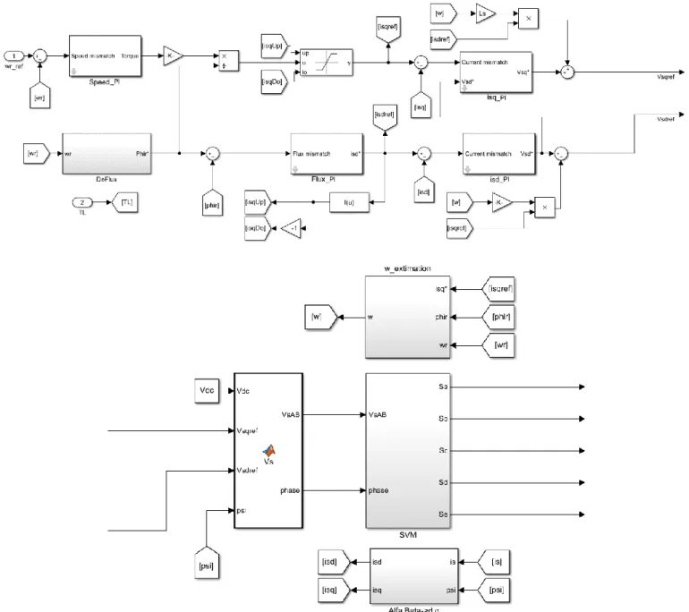
Figure 3.11: Part 2 PWM control Simulink scheme

It is the application of the control model discussed in chapter (2.3.2) to the case of a 5-phase IM.

The PI regulators are tuned with 𝑘𝑝= 0.85𝑘𝑝𝑚𝑎𝑥 and anti-windup is set to 0.5𝑦𝑚𝑎𝑥.

The Speed_PI regulator has a cut-off frequency 𝑓𝑐𝜔_𝑟= 20𝐻𝑧.

The Flux_PI regulator has a cut-off frequency 𝑓𝑐𝜑𝑟= 200𝐻𝑧.

The isq_PI and isd_PI regulators have cut-off frequency 𝑓𝑐𝑖𝑠𝑑𝑞= 2𝑘𝐻𝑧.

In the Switching box a SPWM with a switching frequency 𝑓𝑠= 20𝑘𝐻𝑧 is implemented.

In the VSI box, the matrix (2.40) is implemented with 𝑛 = 5 and 𝑉𝑑𝑐 = 1𝑘𝑉.

In the w_extimation box, the second equation of (2.22) is implemented. In the Direct_Extimation box, equation (2.25) is implemented.

(50)

CHAPTER 3:

3.3.1 Simulation

Figure 3.12 shows the rotor speed profile during normal operation.

Figure 3.12: PWM rotor speed profile

The speed profile is the same as the one of the previous case.

The main differences can be noted in the electromechanical torque profile of Figure 3.13 and the stator phase currents plot of Figure 3.14.

Figure 3.13: PWM electromechanical torque profile

The torque profile has the same shape as before but with less ripple due to the different control strategy.

(51)

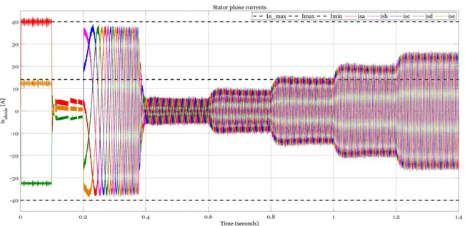
Concerning the stator phase currents their shape is still sinusoidal and symmetric, there’s an increase in magnitude when there’s an increase in the torque and the maximum admissible current for continuous duty 𝐼𝑛𝑚𝑎𝑥, is reached at 0.8𝑠 ≤ 𝑡 < 1𝑠 with less rippled waveforms.

However, the main problem is that the maximum admissible current 𝐼𝑚𝑎𝑥 is exceeded in the

first instants of the simulation.

Figure 3.14: PWM stator phase-currents

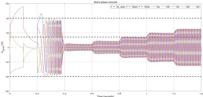
A detail of the stator phase currents is shown in Figure 3.15.

Figure 3.15: PWM stator phase-currents detail

The reason why the limit is exceeded can be found in the stator reference currents 𝛼𝛽𝑥𝑦 plot of Figure 3.16. Of the four currents, only the 𝛼 and 𝛽 components are controlled with a closed loop control, while 𝑖𝑠𝑥 and 𝑖𝑠𝑦 are set to zero with an open loop control. This leads to having a

5-phase induction motor : modeling and control for faulty operations

POLITECNICO DI MILANO

Scuola di Ingegneria Industriale e dell’Informazione

Corso di Laurea Magistrale in Ingegneria Elettrica

5-PHASE INDUCTION MOTOR:

MODELING AND CONTROL FOR FAULTY

OPERATIONS

Relatore:

Prof. Luigi Piegari

Tesi di laurea di:

Marco Andronio

Matricola: 898390

Abstract

Sommario

Contents

List of figures

List of tables

Introduction

CHAPTER 1:

MULTIPHASE MOTOR MODEL

1.1 Magnetic field in the air gap

1.2 Equations

1.2.1 Electrical equations

1.2.2 Mechanical equations

1.2.3 Complete model

1.3 Case study: 5-Phase IM

1.3.1 Model in term of fluxes

CHAPTER 2:

CONTROL MODEL

2.1 Controls

2.2 PI regulators

2.3 RFOC

2.3.1 Control in current

2.3.2 Control in voltage

2.4 n-Phase VSI

CHAPTER 3:

NORMAL OPERATION (NO)

3.1 Motor model

3.2 HR control (NO)

3.2.1 Simulation

3.3 PWM control (NO)

3.3.1 Simulation