A CPU power model for dynamic thermal simulation under benchmark stimuli and DVFS control

(1)

POLITECNICO DI MILANO

Master of Science in Automation and Control Engineering Dipartimento di Elettronica, Informazione e Bioingegneria

A CPU power model for dynamic

thermal simulation under benchmark

stimuli and DVFS control

Relatore: Alberto Leva

Correlatore: Federico Terraneo

Tesi di Laurea di:

Vitaliy Pakholko, 898437

(2)

(3)

Abstract

In modern microprocessor technology there is a strong need for better thermal management. The dark silicon phenomenon makes it impossible to keep active all processing units of a commonly cooled chip without incurring in thermal runaway. Consequently, whenever a core is critically heated the whole chip experiences a frequency throttle-down regarldless of individual temperatures to safeguard the chip’s safety. This frequency down tuning results in significant overall performance losses. The problem is, therefore, two-faced. There is a need for more efficient, lightweight and fast responsive frequency-control schemes that don’t affect all cores indiscriminately. There is also the necessity for a robust testing platform where to test these schemes without risking the processor’s health or employing exotic cooling solutions. In the literature it is already possible to find sofisticated control schemes but their efficacy is only tested in simulation - as physical testing is often problematic - so the need for a testing platform is paramount. A reasonable example of such testing platform is to utilize a thermal test chip (TTC) that, supplied with a proper model, mimics a CPU’s power dissipation under stress. The scope of this thesis is creating such a model by identifying and estimating the relative parameters via a series of ad-hoc benchmarks and tests. Following the identification and estimation process, the model’s simulation is then validated by comparing it with a real processor’s power consumption.

(4)

Sommario

Nelle tecnologia riguardante i microprocessori moderni c’è un forte bisogno di una migliore gestione termica. Il fenomeno del ”dark silicon” rende impossi-bile il mantenere attivi a lungo tutti i componenti di un processore raffreddato con mezzi comuni, senza incorrere in una fuga termica. Di conseguenza, og-niqualvolta uno dei core è riscaldato a livelli critici, l’intero chip subisce un calo di frequenza per prevenire danni al chip stesso. Questo abbassamento delle frequenze produce quindi un calo generale della performance del processore. Dunque il problema è duplice. Da una parte c’è bisogno di un più efficiente, leggero e veloce schema di controllo della frequenza che non coinvolga indis-criminatamente tutti i cores del chip. Dall’altra c’è anche la necessità per una piattaforma per analisi dove si possano testare questi schemi di controllo senza rischiare la sicurezza del chip od impiegare sistemi di raffreddamento esotici. Nella letteratura è già possibile trovare schermi di controllo sofisticati ma la loro efficacia è comprovata solamente in simulazioni - in quando analisi fisiche risultano spesso problematiche - quindi il bisogno di una piattaforma di analisi `

e di primaria importanza. Un ragionevole esempio di tale piattaforma `e realizz-abile tramite l’impiego di un ”thermal test chip” (TTC) che, con l’ausilio di un opportuno modello, ricalca la dissipazione termica di un microprocessore sotto stress. Lo scopo di questa tesi `e di creare un tale modello tramite la stima e l’identificazione dei relativi parametri con l’ausilio di una serie di esperimenti e benchmarks realizzati ad-hoc. In seguito al processo d’identificazione e stima, segue una validazione del modello comparandolo con dati di consumo energetico di un processore reale.

(5)

Ringraziamenti

Ringrazio il Professor Leva per avermi dato l’opportunit´a di lavorare su questa interessante tesi, Ing. Terraneo per avermi assistito ed Antonella per il supporto morale durante questi anni.

(6)

List of Figures

3.1 Supply voltage measurement circuit . . . 19

3.2 Current measurement circuit . . . 20

3.3 Power dissipation dynamic with BurnP6 command . . . 22

3.4 Power dissipation dynamic with Highload command . . . 22

3.5 Power dissipation dynamic, cache-miss and BurnP6, half period each . . . 22

3.6 Power dissipation dynamic, incremental active core count . . . . 23

3.7 Power dissipation dynamic after l=0 for all cores, temperature decreasing . . . 24

3.8 Leakage power related to CPU temperature . . . 25

3.9 Power dissipation dynamic at 1625MHz, BurnP6 . . . 26

3.10 Power dissipation dynamic at 3500MHz, BurnP6 . . . 26

3.11 Core voltage dynamic during leakage test . . . 28

3.12 CPU core voltage measurement . . . 28

3.13 Power dissipation dynamic, model vs data, BurnP6, 2375MHz . . 29

(9)

List of Tables

(10)

Chapter 1

Introduction and related

work

1.1 Introduction

In the microelectronics sector, the importance of thermal optimization and com-puting efficiency is of ever-increasing importance. Given the tremendous amount of information processed on an everyday basis, even the slightest improvement results in a significant output difference and considerable power savings.

Modern CPUs have multiple cores and the power density is high enough to make it impossible to run them simultaneously at full power, thus, hurting the overall computational performance [1]. For many years, in the single core computers era, microprocessors benefitted from Moore’s and Dennard’s laws increasing frequency and density while benefitting from a decreasing dissipated power. After the breakdown of Dennard’s scaling in 2005, the CPU designers’ attention turned to increasing the number of cores to maintain the Moore’s law instead of focusing on single core performance [2]. With time, the number of transistors and cores on a chip increased as well as the power consumption while the heat dissipation strategies could not keep pace; this problem is well known in the industry and is called dark silicon[3, 4]. The higher power consumption stemmed from the impossibility to further reduce the CPU’s operating voltage below around 1 volt, while the continued scaling and increase in the number of transistors resulted in an increase in power and power density. These facts re-sulted in the necessity of using frequency as a mean to control heat production,

(11)

avoiding damage by thermal runaway to the chip when the heat dissipation was not enough. De facto this also meant that while only certain cores had to be throttled down to avoid thermal failure, all the cores suffered from decreased performance [1, 2, 3].

1.2 Problem statement

There are already frequency control oriented solutions for synchronous CPUs proposed to tackle this problem, utilizing, for example, clock gating techniques [5] to throttle only the critically heated processing units but the proprietary software-hardware bundle makes it impossible to control individual cores; the only way to validate results were software simulations.

In order to test the physical viability of such solutions, while ignoring the constraints of a multi-layer proprietary system, it would be needed to connect the processor chip to a custom-made test bench with full control for voltage, current, frequency and the possibility to measure temperature accurately. In such test conditions the chip is much more likely to experience critical failures due to removal of all the safety systems present in modern motherboards, mak-ing it a potentially expensive and therefore undesirable method.

A safer and less expensive testing method would be employing thermal test chips (TTC from now on), commercial devices which purpose is to dissipate power in a controlled manner. The main drawback for our purpose of testing frequency-oriented solutions is that TTCs are the equivalent of resistive loads and thus frequency invariant. On the other hand, these types of chips are advan-tageous since it is possible to selectively heat areas, mimicking the heated core problem and contrarily to commercial CPUs, we have an array of temperature sensors in well known locations thus having a potentially better measurement.

In our case, we would need to impose a time variable power output to the TTC in the form of a time variable 4x4 power matrix for example, which will resemble a typical CPU workload with known frequency, temperature, voltage and current. Each equivalent of a physical core will then have its dissipated power at its virtual running frequency; in this way it will be possible to test any thermal control solution on the TTC.

(12)

In order to make these tests relevant we should make sure that these ther-mal power responses are as true to reality as possible by creating and running a series of benchmark thought to stress the CPU at various frequencies and reg-istering the thermal output tracks. The goal of this thesis, thus, is to create a simple but effective frequency dependant thermo-electrical model that will allow the testing of frequency dependant control strategies on a resistive thermal chip.

1.3 Related work

The dark silicon problem introduced the need for better thermal control strate-gies in order to counteract the need to dim a portion of the chip to maintain thermal safety. Such strategies tried to integrate thermal and performance man-agement and, as for example [5] presents, ranged from LQR, MPC to convex optimization and extremum seeking. Other solutions like [5] itself and [7], use an event-based approach instead, in an attempt of reducing the computational stress of the control itself while also improving its response time. It is important to note that since the control is executed by the CPU itself and not an external device, the control scheme must be as simple and computationally lightweight as possible to guarantee responsiveness and low power consumption with respect to the actual workload. In order to effectively test the price-performance ratios and effectiveness of these methods, there is a need for a general physical test platform with as less hardware and software constraints as possible.

There are different approaches that attempt to tackle this problem in the literature, for example instead of using a TTC in [4], a delidded processor is employed. In this experiment, an infrared-transparent oil is used for cooling purposes and a thermal camera to precisely measure the temperature distribu-tion on the chip. The advantage of this method with respect to a TTC is the possibility to run performance benchmarks on the same device that will perform the workload, thus eliminating the need for a parametrized dissipation model but the big drawback is the impossibility to use any other cooling system ex-cept this specific exotic solution employed. The fact that a TTC supported by a proper model can employ any cooling solution makes it much more relevant for tests of control schemes designed for general use, as most existing processors employ a wide range of generic cooling solutions.

(13)

In order to take advantage of the TTC technology, it is needed to develop a power dissipation model for the CPU, thus involving frequency, but still applica-ble to a resistive load. It is also worth noting that by such design we are enaapplica-bled to test controllers against any community designed benchmark, further increas-ing the importance of the thesis. In the literature there already exist various models that can be used in the scope of this thesis, in particular [6] takes into account both leakage, dynamic power and the utilization factor “alfa” which is particularly fitting in the context of processors performing complex tasks like in our case, explained in the model section.

1.4 Organization

The dissertation is organized as follows:

• Chapter 2 presents the overall model and the relative parameters, jus-tifying in each subsection the assumptions we made about leakage and dynamic power cited in the bibliography ;

• Chapter 3 describes the parameters estimation process and presents the tests involved with relative results;

(14)

Chapter 2

Modelling and

parametrization

As anticipated in chapter 1, our goal is to create a CPU power dissipation model in order to recreate a power response dynamic on a TTC as true to reality as possible. In order to achieve such a model, we needed to highlight the role of frequency in the power output; additionally, in modern microprocessors, signif-icant amounts of power are lost to current leakage phenomena [10] and thus played a primary role in the model as well, as shown below.

2.1 System information

To be able to reach our target we will use the available knowledge cited in the previous chapter and adapt it to the current physical system comprised by an intel i5-6600k processor, corsair 650W power supply and asus z170 motherboard.

As the system we are treating is inclusive of an overclockable processor, we must highlight the motherboard’s components that may be relevant for our hy-potheses and the resulting model.

A phase locked loop (PLL) is present, a frequency control device which sets the clock as a product of base frequency x desired multiplier. It is important for us to be able to manually set a constant frequency for the full duration of

(15)

benchmarks with no intrusion by external agents so we took full advantage of this component.

The dynamic voltage and frequency scaling (DVFS) mechanism serves to maintain the system in optimal working conditions under any frequency varia-tion. Since modern CPUs are comprised mostly from CMOS transistors, each node has a certain parasite capacitance (gate, diffusion and/or coupling capac-itances) [6] that needs to discharge and recharge each time switching occurs. As we know, capacitances’ charge rates are proportional to the applied voltage and thus we must consider that higher frequencies require higher voltages to maintain system stability. To further clarify, in order for a system composed by transistors to be considered stable, the logic ports’ delay must be below a certain fraction of clock period; as this delay is inversely proportional to voltage as stated above, higher clock frequencies require higher voltages.

There are two other hardware entities that may interfere with our modelling – intel’s Turbo boost technology and integrated graphics – and as such we dis-abled or compensated for them if we could. In the integrated graphics’ case, it was impossible to completely disable it, so we tried to take account of its effect on the power consumption to the best of our possibilities.

2.2 Hypotheses

Considering the information avaiable about the system we decided to use a sim-ple model for the power output similar to [6], consisting of the sum of the power lost to leakage and the dynamic power component. More complex models were also been considered, like for example the one shown in [11] which comprises also the power lost to short circuit conduction - but - due to lack of precise architectural knowledge we decided to use simpler models to avoid overfitting. For example, it is not possible for us to establish the amount of power lost by the integrated GPU of the intel’s chip, therefore, the addition of ulterior terms in the formula was not beneficial and it was modelled as part of the leakage term. Further considerations on model expansion are discussed in the conclusions and future work chapter 4.

(16)

Temperature wise, it was not possible for us to set up an accurate and independent measuring system without delidding the microprocessor and con-siderably complicate the structure of the test bench. Considering this fact and the role of temperature in our model, we decided to assume the embedded sen-sors as accurate enough for the scope of our tests.

2.3 Model

The resulting grey box model has the simple form of

Ptot(t) = Pleak(t) + Pdyn(t)

components of which will be expanded in the following subsections, while the composing parameters will be explained in the parametrization section.

2.3.1 Leakage power

The first addend - leakage power - is the power lost due to transistor inefficien-cies. Ideally when a MOSFET is in the off state there should be no current flow but, in a real transistor, a small number of electrons will be circulating through the gate and between and semiconductor junctions.

The gate leakage occurs due to the quantum tunnelling phenomenon [8], it increases exponentially as the insulating region decreases and as such it’s one of the main limiting factors for higher transistor density on modern chips.

Leakage can also occur between the carriers of the MOSFET (source and drain) being called in this case subthreshold conduction – or also – between the interconnects.

The leakage power is modelled as

Pleak(t) = V (t) I0e

T (t) T0

and most importantly for our case, as highlighted in [6, 9], leakage increases exponentially with temperature, thus the presence of the exponential factor. It is worth noting that leakage power is linear with respect to the voltage but the nonlinear part is strongly influenced by the yet unestimated T0parameter.

(17)

2.3.2 Dynamic power

As stated in the DVFS explanation, each time a transistor changes its state, there is a charge or discharge of its internal parasite capacitance; during this transient there is a power loss proportional to the capacitance itself, to the switching frequency and quadratically proportional to the voltage.

It is also estabilished that dynamic power is also dependant on which opera-tion the CPU is performing. As stated in [5, 6, 7], there is a difference between an operation employing a lower amount of transistors like a cache miss and a more intensive ad-hoc process like cpu-burn, additionally the core can be com-pletely idle during fractions of the test. This variance in output is included in the model in the form of two additional time depending factors of α(t) and l(t), described in the parametrization section. The resulting power loss, therefore, is modelled as

Pdyn(t) = C0f V (t)2α(t) l(t)

This strong voltage dependence suggests that lower values are very advan-tageous for power consumption but also negatively affects system stability as stated in the DVFS paragraph so we decided to run all the test with values above 1,4 V.

2.4 Parametrization

Being our resulting model

Ptot(t) = V I0e

T (t)

T0 _{+ C}₀_{f V (t)}2_{α(t) l(t)}

We will separate these parameters in measurable and derivable.

2.4.1 Measurable

• f is measured in Hertz and is the frequency at which the transistors in the cores are switching. It is not only measurable, but we can impose it to any reasonable value by setting the frequency multiplier, taking advantage of the PLL. In our model, it linearly increases dynamic power losses as implied above but has no repercussion to leakage power;

• T is the core temperature and is measured in Kelvin degrees. Its measure-ment is entrusted to the embedded sensors present on the silicon itself;

(18)

• V (t) is the core voltage and it’s measured by an acquisition card down-steam the voltage regulator commanded by the DVFS. The choice not uti-lizing the built-in sensor is dictated by the difficulty of real time reading without affecting the test itself – we tried force the CPU cores to execute our test process with less interruptions possible – so external measurement was the most reasonable solution. It is worth noting that this value was expected to remain constant when performing tests at a steady frequency but experienced load induced variations. A possible explanation will be presented in the results section.

2.4.2 Derivable

• T0 and I0 are supposed to be constant and have the dimensions of a

temperature in Kelvin and a current in Ampere and will be targets of our parameter identification analysis;

• C0 is a parameter and is the equivalent capacity parameter expressed

in Farad. Ideally this parameter is constant but some variation of this parameter due to temperature is expectable;

• α(t) is the normalized utilization factor of the CPU ranging from 0 to 1. In the parametrization chapter, it will be proven that not all micropro-cessor instructions provide the same power output and this parameter is introduced to take into account this inequality;

• load l(t) is a two state flag which indicates if the core is powered or not; therefore if summed during an interval, it takes the shape of a real value representing the average amount of time the core was active during such interval.

(19)

Chapter 3

Parameters’ identification

process and results

In this section we are going to define the test bench components and explain the methods or experiments we employed to identify our model’s parameters.

3.1 Test bench composition

Our test bench is built as follows:

• Intel core i5-6600K CPU with stock cooler and cooler master thermal paste;

• Asus z170 motherboard with customized bios settings. Unlocked frquency multiplier with base clock being 125MHz and multiplier ranging between 8 and 35 across all of our tests. Disabled turbo boost and base clock spread spectrum;

• Corsair VS650 power supply;

• Maxwell technologies amplifier with 25x gain;

• National instruments NI USB-6210 acquisition card;

• No dedicated GPU, DVD readers or any device not fundamental for the correct functioning of the test bench.

(20)

3.2 Methodology

As stated in the Model section, the dissipated power can be represented as the function

Ptot(t) = g(V (t), T (t), f (t), α(t), l(t), C0, T0)

The first part of the process is to showcase the measuring process for the cor-responding - measurable - variables for then to proceed to the, more relevant, estimation process.

3.2.1 Measuring of total power loss

In order to obtain the total dissipated power, it was deemed sufficient to mea-sure the supplier’s voltage and delivered current through the 12V line.

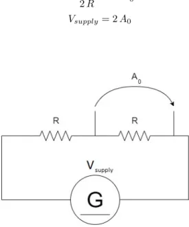
In order to obtain the voltage, we attached a simple circuit in parallel to the power supplier’s 12V cable pins. Since our acquisition card could only handle up to 6V, we used a voltage divider composed of two equal resistors and measured the voltage drop on one of them; we then re-obtained the real voltage by simply doubling the measurement later, via software means. We will refer to this value as Vsupply from now on. Formulas in this subsection refer to instantaneous

val-ues, thus dependancy from time will be dropped for the time being.

VsupplyR

2 R = A0 Vsupply = 2 A0

(21)

The current measurement was obtained by inserting a 0.01 Ohm 4 terminal resistor coupled with an amplifier between the power supply and the mother-board (G0=25). Since the resistor is of such small impedance, no current loss

due to measurement is expected; while the amplifier is used to ensure that the small voltage drop is read more precisely by the acquisition board. This current will be called Isupply and is obtained with

Vr= RcIsupply = 0.01[Ω] Isupply

A0= VrG0= 0.25[Ω] Isupply

Isupply = 4 A1

.

Figure 3.2: Current measurement circuit

It was also assumed that power losses due to motherboard activity or cable resistance were negligible and therefore the CPU power dissipation would be simply

Ptot= VsupplyIsupply = 8 A0A1

3.2.2 Measuring of core voltage and temperature

The core voltage value was obtained via the measuring of the differential tension between of the pins of the voltage regulator capacitance. We assumed that the equivalent resistance between the capacitor and the CPU cores was negligible -the implication of this hypo-thesis will be shown in -the results section 3.3.

(22)

Core temperature was measured simply taking advantage of the embedded sensors.

3.2.3 Estimation of the utilization factor α

In order for our final model to produce meaningful results, we needed to confirm the existence of the utilization factor and showcase how it affects the power consumption. In order to do so, two kind of tests were performed:

• a first test in which we executed various commands meant to maximumly stress the CPU at the nominal base frequency provided by the manufac-turer. We expected that the most power consuming process would result in a power consumption equal to the thermal design power (TDP). If such a command existed, we would use it for all of us tests, as it would cor-respond to an α equal to 1, de facto eliminating one parameter from the equation;

• a second test in which we would use a command that theoretically has a low α alternating periodically with a high α process. If such test would result in a power response resembling a square wave, we could validate the existence and importance of the utilization factor.

As goes for the first test, two scripts generated the highest power consump-tion - one employing repeated multiplicaconsump-tions with the same factors without writing the result in memory (HighLoad) and the other being BurnP6 - each with own advantages and disadvantages.

We can see in figure 3.3 the Highload’s induced power output is much less noisy but BurnP6 is very close to TDP of 91W provided by the manufacturer, thus we decided to use it in all of our tests and will assume α as 1.

As for the second test (figure 3.4), we chose a script utilizing a cache miss simulation as the lower α process. Theoretically the CPU is not performing computations while waiting for the cache to fetch new data and thus we expect a lower utilization factor. For the high α process, we employed BurnP6 from above.

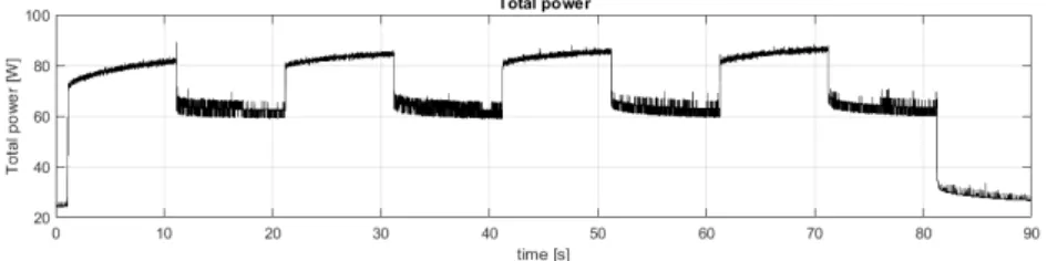
In figure 3.5 it is clearly shown that we have obtained a square wave-like power output with significant difference between high and low state, hence, validating our initial hypotheses about the significance of the utilization factor.

(23)

Figure 3.3: Power dissipation dynamic with BurnP6 command

Figure 3.4: Power dissipation dynamic with Highload command

Figure 3.5: Power dissipation dynamic, cache-miss and BurnP6, half period each

(24)

3.2.4 Estimation of the load factor l

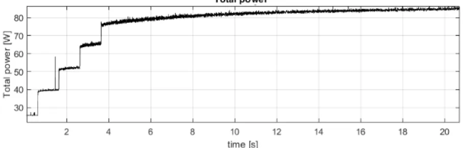
The load factor l indicates if the core is powered or not, therefore has only two states: 0 and 1. We will show the effect of BurnP6 starting from a single core then gradually initializing it on all 4.

Figure 3.6: Power dissipation dynamic, incremental active core count

In figure 3.6 it is visible that each core has around equal contribution as expected. It is worth anticipating that when all cores are not executing any stressful process - even if there will always be unavoidable operating system activity - Pdyn is assumed equal to zero, thus, Ptot will be comprised solely of

Pleak.

3.2.5 Estimation of leakage current I

0

As anticipated in the previous subsection, we can isolate Pleak by not running

any process during our tests leaving us with

Ptot(t) = Pleak = V (t) I0e

T (t) T0

thus

Ptot(t) = h(V (t), I0, T (t), T0)

(25)

In order to do so, we devised an experiment consisting in heating the chip to nearly the maximum allowed temperature of 100 degrees Celsius, then stop-ping all processes and observing the power output curve while temperature was logged and the processor cooled down. The resulting power output is shown in figure 3.7

Figure 3.7: Power dissipation dynamic after l=0 for all cores, temperature de-creasing

As we acknowledged that there is indeed a relationship between leakage cur-rent and temperature, we proceeded to verify the correctness of our leakage model. Using modern solvers, and by combining data from the temperature sensor and the core voltage, we estimated the I0 and T0 parameters using the

extremes of the curve as data points. We then followed by building a temper-ature to leakage-power graph with data and compared it with the estimated equivalent in figure 3.8.

(26)

Figure 3.8: Leakage power related to CPU temperature

Despite the apparent noisiness and increased density around the lower end of temperatures - since it’s not a function but a collection of data points - it can be clearly seen as a proper fit of exponential type. We will further validate this part of the model in the final subsection.

3.2.6 Estimation of equivalent capacitance C

0

With new information available from the estimation of Pleak we were now able

to tackle the dynamic power problem. As a reminder

Pdyn(t) = C0f V (t)2α(t) l(t)

where V (t) is measured, α and l can be considered equal to 1 if BurnP6 is exe-cuted on all cores.

In order to estimate C0 we executed BurnP6 stress tests, each time, with a

different imposed frequency. In order to truly be independant from the Pleak

dynamic, each test is of duration of at least 180s in order to reach a stable temperature value. Two examples of this tests are shown in figure 3.9 and 3.10.

(27)

Figure 3.9: Power dissipation dynamic at 1625MHz, BurnP6

Figure 3.10: Power dissipation dynamic at 3500MHz, BurnP6

In the last 50 seconds the power curve can be considered at steady state.

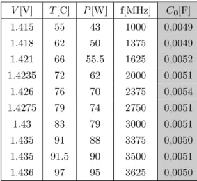
In order to be scrupulous, we performed 10 tests ranging from 1000MHz to 3625MHz while logging the relative Ptot, V (t), and T (t) values.

C0 is then calculated as

C0=

Ptot− Pleak

f V2

and obtained the results depicted in table 3.1, averaging C0=0.0051 F with a

(28)

V [V] T [C] P [W] f[MHz] C0[F] 1.415 55 43 1000 0,0049 1.418 62 50 1375 0,0049 1.421 66 55.5 1625 0,0052 1.4235 72 62 2000 0,0051 1.426 76 70 2375 0,0054 1.4275 79 74 2750 0,0051 1.43 83 79 3000 0,0051 1.435 91 88 3375 0,0050 1.435 91.5 90 3500 0,0051 1.436 97 95 3625 0,0050

Table 3.1: Estimated C0 parameter at respective measured data points

3.3 Results

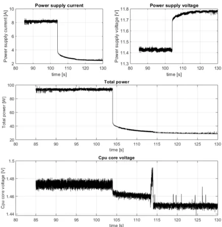
As stated in 3.2.2, we assumed that core voltage is constant due to the relative low value of the resistance between the capacitor anche the CPU. This statement is not completely true, as the voltage we measured varied itself in a step-like manner depending on the CPU load and measured temperature as shown in figure 3.11.

The figure highlights the relationship between core voltage, temperature and load but the voltage drop is so small that the initial hypothesis is still considered valid. The probable reason of this dynamic behaviour is that the DVFS must compensate for the voltage drop occuring on the resistance between the CPU cores and the capacitor (figure 3.12) in order to keep core voltage constant; this explains the step like response since the current also shows a downward step during the load and temperature reductions.

(29)

Figure 3.11: Core voltage dynamic during leakage test

(30)

After having estimated all the necessary parameters, we could then compare the physical results from the tests to a model’s simulation.

To do so, we superimposed

Ptot(t) = Vsupply(t) Isupply(t)

with

Ptot(t) = V (t) I0e

T (t)

T0 _{+ C}₀_{f V (t)}2_{α(t) l(t)}

with data collected at various frequencies, as shown for example in figures 3.13 and 3.14.

(31)

Figure 3.14: Power dissipation dynamic, model vs data, BurnP6, 3375MHz

The figures show a remarkable match between reality and simulation at any frequency and temperature, strongly suggesting the robustness of our power dissipation model. There’s also a slight mismatch in the fist seconds during the gradual activation of BurnP6 on all processing units; it happens because we did not account for the cores activating gradually in the data crossing script but assumed all cores were active from the start, thus, having an overestimation of output power until all units were processing.

It is possible now to rewrite the model in function of only of the measurable parameters:

Ptot(t) = V (t) 0.37[A] e

T (t)

79[K] _{+ 0.0051[F ] f V (t)}2

(32)

Chapter 4

Conclusions and future

work

4.1 Conclusions

The relatively simple model of the CPU’s power consumption under stress fac-tors has proved itself as an excellent approximation of the physical system. In chapter two, we hypothesized that including short circuit conduction and un-known integrated graphics activity into the leakage power term, could result in suboptimal results across different frequencies; given the very limited model error we can safely state that either these phenomena were very limited and thus negligible - or - simply very well approximated by the power leakage model itself. It is important to note that our results apply to a specific processor model - Intel i5-6600K - as for different CPUs correspond different transistor density, different core counts, the presence or lack of integrated graphics etc. and thus overall different internal architecture.

4.2 Future work

A possible example of future work would be testing and extending the model to different CPU architectures by building a database of the newly estimated parameters, enabling in such a way the simulation of a wide range of processors. Alternatively it could be advantageous to construct a new - less precise - model,

(33)

starting from this one, in order to obtain a general model, agnostic to the CPU model in use.

We can conclude this dissertation by stating that the model is ready to be taken advantage of for testing purposes, for example in conjunction with a TTC device as stated in the problem statement section.

(34)

Bibliography

[1] J. Henkel, “Dark silicon - a thermal perspective”, in Proceedings of Tech-nical Program - 2014 International Symposium on VLSI Technology, Sys-tems and Application (VLSI-TSA), 2014, pp. 1–1. doi: 10.1109/VLSI-TSA.2014.6839641.

[2] H. Esmaeilzadeh, E. Blem, R. S. Amant, K. Sankaralingam, and D. Burger, “Dark silicon and the end of multicore scaling”, in 2011 38th Annual In-ternational Symposium on Computer Architecture (ISCA), 2011, pp. 365– 376.

[3] F. Terraneo, A. Leva, and W. Fornaciari, “Event-based thermal control for high power density microprocessors: A cross-layer approach”, in. Jan. 2019, pp. 107–127, isbn: 978-3-319-91961-4. doi: 10.1007/978-3-319-91962-1_5.

[4] A. Leva, F. Terraneo, and W. Fornaciari, “An open-hardware platform for mpsoc thermal modeling”, in Embedded Computer Systems: Architec-tures, Modeling, and Simulation - 19th International Conference, SAMOS 2019, Samos, Greece, July 7-11, 2019, Proceedings, D. N. Pnevmatikatos, M. Pelcat, and M. Jung, Eds., ser. Lecture Notes in Computer Science, vol. 11733, Springer, 2019, pp. 184–196, isbn: 978-3-030-27561-7. doi: 10 . 1007 / 978 - 3 - 030 - 27562 - 4 \ _13. [Online]. Available: https : / / doi.org/10.1007/978-3-030-27562-4\_13.

[5] D. Mirco, Event-based power-performance-thermal management with task migration in high-power cpus, 2018.

[6] N. S. Kim, T. Austin, D. Baauw, T. Mudge, K. Flautner, J. S. Hu, M. J. Irwin, M. Kandemir, and V. Narayanan, “Leakage current: Moore’s law meets static power”, Computer, vol. 36, no. 12, pp. 68–75, 2003, issn: 1558-0814. doi: 10.1109/MC.2003.1250885.

(35)

[7] A. Leva, F. Terraneo, I. Giacomello, and W. Fornaciari, “Event-based power/performance-aware thermal management for high-density micro-processors”, IEEE Trans. Contr. Sys. Techn., vol. 26, no. 2, pp. 535–550, 2018. doi: 10 . 1109 / TCST . 2017 . 2675841. [Online]. Available: https : //doi.org/10.1109/TCST.2017.2675841.

[8] A. Seabaugh, “The tunneling transistor”, IEEE Spectrum, vol. 50, no. 10, pp. 35–62, 2013, issn: 1939-9340. doi: 10.1109/MSPEC.2013.6607013. [9] S. Mukhopadhyay, A. Raychowdhury, and K. Roy, “Accurate estimation

of total leakage current in scaled CMOS logic circuits based on compact current modeling”, in Proceedings of the 40th Design Automation Confer-ence, DAC 2003, Anaheim, CA, USA, June 2-6, 2003, 2003, pp. 169–174. doi: 10.1145/775832.775877. [Online]. Available: https://doi.org/ 10.1145/775832.775877.

[10] S. Naffziger, “High-performance processors in a power-limited world”, in 2006 Symposium on VLSI Circuits, 2006. Digest of Technical Papers., 2006, pp. 93–97. doi: 10.1109/VLSIC.2006.1705327.

[11] H. Sultan, G. Ananthanarayanan, and S. R. Sarangi, “Processor power estimation techniques: A survey”, IJHPSA, vol. 5, no. 2, pp. 93–114, 2014. doi: 10.1504/IJHPSA.2014.061448. [Online]. Available: https://doi. org/10.1504/IJHPSA.2014.061448.

[12] D. N. Pnevmatikatos, M. Pelcat, and M. Jung, Eds., Embedded Com-puter Systems: Architectures, Modeling, and Simulation - 19th Interna-tional Conference, SAMOS 2019, Samos, Greece, July 7-11, 2019, Pro-ceedings, vol. 11733, Lecture Notes in Computer Science, Springer, 2019, isbn: 978-3-030-27561-7. doi: 10.1007/978- 3- 030- 27562- 4. [Online]. Available: https://doi.org/10.1007/978-3-030-27562-4.

A CPU power model for dynamic thermal simulation under benchmark stimuli and DVFS control

POLITECNICO DI MILANO