UNIVERSITY OF PISA
The School of Graduate Studies in Basic Sciences "GALILEO GALILEI"
Ph. D. T H E S I S
Measurement of the inclusive jet
cross section with the ATLAS
detector at the LHC
Candidate:
Advisor:
Jury :
Reviewers : Franco BEDESCHI - INFN - Pisa
Jonathan BUTTERWORTH - Univerity College London
Gavin SALAM - CERN; Princeton University;
LPTHE, UPMC Univ. Paris 6 and CNRS Advisor : Chiara Maria Angel RODA - University of Pisa and INFN - Pisa
President : Kenichi KONISHI - University of Pisa
Examinators : Elisabetta BARBERIO - University of Melbourne
Franco BEDESCHI - INFN - Pisa
Mauro DELL’ORSO - University of Pisa
Contents
1 The ATLAS experiment at the Large Hadron Collider 5
1.1 The Large Hadron Collider at CERN . . . 5
1.1.1 A brief history . . . 5
1.1.2 The accelerator chain . . . 6
1.1.3 Delivered luminosity . . . 7
1.2 The ATLAS detector . . . 11
1.2.1 Inner Detector . . . 12
1.2.2 Calorimetric system . . . 15
1.2.3 The muon spectrometer. . . 20
1.2.4 Trigger and Data acquisition . . . 21
1.2.5 Monte Carlo simulation of the ATLAS detector . . . 24
1.2.6 The data samples collected in 2010 . . . 24
2 Jet production at hadron colliders: Theoretical predictions 27 2.1 Fundamental interactions: the Standard Model. . . 27
2.2 The Strong interactions: the Quantum Chromo-Dynamics (QCD) . . . 30
2.2.1 Structure of pQCD predictions . . . 30
2.2.2 From the soft divergences to the jet algorithms . . . 33
2.2.3 Beyond the fixed order predictions: the parton shower and non per-turbative effects. . . 38
2.2.4 Different strategies to get a predictions . . . 41
2.3 Inclusive jet cross section: Theoretical prediction . . . 43
2.3.1 Fixed order pQCD . . . 44
2.3.2 Total theoretical uncertainties for the fixed order predictions . . . . 50
2.3.3 NLO Matrix Element + Parton Shower . . . 51
3 Measuring jets: Reconstruction and Calibration 53 3.1 Jet reconstruction . . . 53
3.1.1 Jet inputs . . . 54
3.1.2 Jet calibration procedure: EM+JES . . . 54
3.2 Jet algorithms: back to definitions . . . 60
3.2.1 Reconstruction efficiency and purity . . . 60
3.2.2 Picking up all the high energy objects: the dark clusters. . . 63
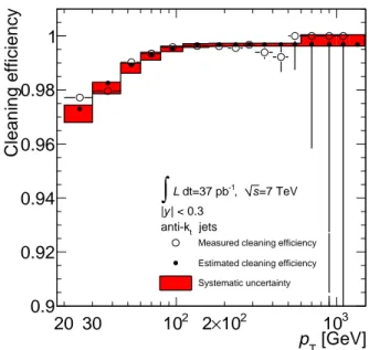
4 Measuring jets: Performancies 69 4.1 Jet cleaning . . . 70
4.3 Jet energy calibration . . . 75
4.3.1 Jet energy scale: from the calorimetric response to an isolated hadron to the final estimate of the uncertainty . . . 75
4.3.2 Jet energy resolution . . . 99
5 The inclusive jet cross section: Measurement with 37 pb−1 103 5.1 Trigger and luminosity . . . 104
5.1.1 Trigger strategy . . . 104
5.1.2 Luminosity . . . 108
5.2 Event and jet selection . . . 110
5.2.1 Jet selection . . . 111
5.2.2 Data stability . . . 111
5.3 Correcting the detector effects: unfolding . . . 111
5.3.1 Monte Carlo samples for the unfolding . . . 112
5.3.2 Detector level shape: improving the Monte Carlo descriptions . . . 113
5.3.3 Unfolding strategy . . . 115
5.3.4 Computing the statistical uncertainty with the IDS unfolding . . . . 116
5.3.5 Systematic uncertainty on the unfolding procedure . . . 117
5.3.6 Comparison between IDS and bin-by-bin unfolding . . . 118
5.4 Systematic uncertainties . . . 120
5.4.1 Uncertainty on the jet energy scale . . . 120
5.4.2 Uncertainty on the jet energy resolution . . . 123
5.4.3 Total systematic uncertainty . . . 124
5.4.4 Correlations. . . 125
5.5 Results. . . 129
6 Conclusions 145 A Comparison of the 2010 Summer result and the complete 2010 data analysis 147 B Additional material to Chapter 2 151 C Additional material to Chapter 4 159 C.1 Jet cleaning . . . 159
D Additional material to Chapter 5 169
Introduction
The measurement of the inclusive jet cross section is one of the test of perturbative quantum chromo-dynamics par excellence. The jets, sprays of particles, are copiously produced in the high-energy proton-proton collisions, such at the one at the Large Hadron Collider. They are the footprints of the interactions of quarks and gluons, under the influence of the strong force. The measurement of the inclusive jet cross section depends on the value of the strong force coupling constant, on the structure of the proton, and on the dynamics of the strong force in a large variety of regimes.The major distinctive features of the inclusive jet cross section reported in this thesis with respect to previous measurements carried out at other high energy colliders are:
• the measurement can profit of the unprecedented collision intensity and
center-of-mass energy of √s= 7 TeV provided by the Large Hadron Collider, overcoming
the highest transverse jet momentum measured in previous experiments by a factor larger than two;
• the wide solid angle coverage of the ATLAS experiment allows the measurement of the cross section in uncharted angular regions;
• the quality of the ATLAS measurement of jets at low energies allows the extension of the cross section measurement to really low energy;
• the jet cross section profits of the new anti-kt jet definition developed in the last
couple of years. The choice of this jet algorithm overcomes the problems in the data-prediction comparison caused by previously used jet algorithms.
All these features make the presented jet cross section, one of the more extensive and detailed measurement of the jet physics at hadron colliders. The ATLAS Collaboration prepared a first public result on the inclusive jet cross section, reported in Reference [ATLAS Collaboration 2011k]. These preliminary results have been used as a starting point for the analysis discussed in this thesis, that has largely improved the previous re-sult.
The inclusive jet cross section presented in this thesis is the double-differential cross
section, measured in bin of transverse momentum pT and rapidity |y|. The jet transverse
momentum pTis the component of the jet momentum perpendicular to the direction of the
colliding particles. The jet rapidity is defined as:
y=1
2ln(
E+ pz
E− pz) (1)
where E is the jet energy and pz is the jet momentum along the direction of the colliding
particles. The double-differential inclusive jet cross section is given by:
d2σ
d pTdy
= N
as a function of pT and y. Here N is the number of jets measured in a bin in pT (with a
bin width ∆pT), and y (with a bin width ∆y), and L is the total integrated luminosity. The
inclusive jet cross section is measured for 20 GeV < pT< 1500 GeV, and for −4.4 < y <
4.4, which is the wider range reached so far at hadron collider. The data sample used in
this analysis amounts to an integrated luminosity L of almost 37 pb−1. This is the total
statistics collected in 2010.
The easy definition of the cross section hides the several studies performed in the last years to define a jet, to check the precision of the jet calibration, to correct for the detector effects and finally to take into account in the most complete way all the different sources of systematic uncertainties. These aspects will be discussed along the thesis. It must be clear from the beginning of this report that the list of studies needed to get the final measurement of the inclusive jet cross section, with the detailed and mature results presented in this thesis, represents a challenge not only for a single person, but for a group of people.
The author of this thesis had the possibility to participate to most of the discussions, having a leading role in the measurement of this cross section. The next lines will introduce the structure of the thesis, and the personal contribution to the different parts.
Structure of the thesis and personal contribution
The thesis is divided in 5 Chapters. Chapter1is a short introduction to the Large Hadron
Collider, and to the ATLAS experiment. The author participated to some special operation of the detector as shifter of the hadronic calorimeter TileCal. In particular, he was on shift for the first beams circulating in the Large Hadron Collider in 2008 and for the first
collisions at √s= 900 GeV in 2009. Since May 2011 he is participating to the TileCal
operations as run coordinator.
Chapter2is divided into two parts. The first one (Sections2.1and2.2) is an
introduc-tion to the Standard Model of particle physics and to the quantum chromo-dynamics,
heav-ily inspired to the clear, complete and concise description in Reference [Dissertori 2010].
The second one (Section2.3) is the theoretical estimate of the inclusive jet cross section.
In this section, the author contributed as a responsible for defining the guidelines for the ATLAS Collaboration to estimate the jet cross sections (not only the inclusive jet cross section). In the ATLAS Collaboration, he did the first tests of the NLO predictions with
the anti-kt jet algorithm and the first tests of the Powheg formalism for the jet production.
The major contributions for the inclusive jet cross section have been the cross checks of the theoretical predictions (the fixed order NLO prediction, the non-perturbative correction and the Powheg results). In particular, the author developed part of the code used to derive the non-perturbative corrections.
Chapter3is an introduction to the jet reconstruction in ATLAS. This is divided into
two parts. The first part (Section 3.1) defines the strategy adopted to reconstruct jets in
ATLAS for the 2010 data. On this part, the author gave a contribution to the design of the
JetPerformance package (see Reference [Doglioni 2011b]) in the ATLAS software, used
3.2) describes some experimental aspects in the jet definition, which drove the ATLAS
Collaboration to select the anti-kt jet algorithm as the default jet algorithm for the first
period of data taking. The studies on this topic, done by the ATLAS Collaboration in 2009, cover several aspects. In the section reported in this thesis, only some of the relevant tests, done by the author, are reported.
Chapter 4 describes the performances and the uncertainties in the jet reconstruction.
The Chapter is mostly devoted to the uncertainty on the jet energy scale. In particular, the author gave a contribution in checking the background contribution on the measurement of the calorimeter response to single particles. Another important contribution consists in the development of the selection criteria of events to be used for the multi-jet balance technique. This technique has been used to have an alternative cross check of the precision on the calibration of very high-energy jets.
Chapter 5 gives a detailed description of the measurement of the inclusive jet cross
section. These results would have not been possible without the contributions of almost
thirty people participating at the INCLUSIVEJET ANDDIJETCROSSSECTIONWORKING
GROUPin the ATLAS Collaboration.
The author played a relevant and leading role in this group. He gave a fundamental
contribution in defining the binning of the measurement in pT, especially in the high-pT
region, by checking the impact of the jet energy resolution. He had a leading role in organizing the cut flow and the stability cross checks of the measurement. He provided the detector level spectra in the central region in rapidity used for the unfolded final results. He gave an important contribution on the techniques to propagate the systematics errors on the jet energy scale to the final cross section, cross checking the final bands, and combining the different contribution on the final measurement. He combined the contributions from
INCLUSIVEJET ANDDIJETCROSSSECTIONWORKINGGROUPon the measurement of
the inclusive jet cross section for the ATLAS Collaboration. He was one of the fundamental
authors of the measurement reported in Reference [ATLAS Collaboration 2011k]. He has
been author and editor both of the public note of the measurement reported in Reference [ATLAS Collaboration 2011j] and of the paper (in preparation) containing the results of this thesis.
The ATLAS experiment at the Large
Hadron Collider
Contents
1.1 The Large Hadron Collider at CERN . . . 5
1.1.1 A brief history . . . 5
1.1.2 The accelerator chain . . . 6
1.1.3 Delivered luminosity . . . 7
1.2 The ATLAS detector. . . 11
1.2.1 Inner Detector . . . 12
1.2.2 Calorimetric system . . . 15
1.2.3 The muon spectrometer. . . 20
1.2.4 Trigger and Data acquisition . . . 21
1.2.5 Monte Carlo simulation of the ATLAS detector . . . 24
1.2.6 The data samples collected in 2010 . . . 24
This chapter takes a closer look at the Large Hadron Collider located at CERN, the European Organization for Nuclear Research, and at one of the detectors placed
along its ring: ATLAS, A Toroidal Lhc ApparatuS (described in detail in
Refer-ence [ATLAS Collaboration 2008a]).
1.1
The Large Hadron Collider at CERN
The Large Hadron Collider (LHC) is a circular accelerator located at CERN and designed to collide beams consisting of protons or heavy-ions. It is currently the highest energy
collider in the world since it collided proton-beams at a center of mass energy of√s= 7
TeV. This section describes the LHC in some more details, and the operation conditions
in 2010. A detailed description of the LHC can be found in References [Bruning 2004a,
Bruning 2004b,Benedikt 2004].
1.1.1 A brief history
The LHC circulated its first beams on 10 September 2008, working as a particle storage ring. After nine days, a failure in an electrical connection led to serious damage, stopping the operations until 2009. CERN has spent over a year repairing and consolidating the
machine to ensure that such an incident cannot happen again. The recommissioning of the LHC began in the summer 2009, and successive milestones have regularly been passed since then. The beams have been re-established in LHC in November 2009, after more than one year of stop.
In 2009 LHC produced for the first time collisions at the center of mass energy of√s=
900 GeV. The data recorded in the period of the accelerator commissioning was important to test the performances of the detector, in preparation of the higher energy collisions.
In March 2010, LHC accelerated and collided protons at√s= 3.5 TeV, reaching the
highest beam and collisions energy in the world. The LHC is designed to accelerate and collide particles grouped in trains of bunches. In the first days, only two bunches of pro-tons were injected in the machine, colliding on the four interaction points. The experience gained with the operation and analysis of the first data recorded in 2010 has been mainly directed to the commissioning of the trigger and data acquisition systems and to the under-standing of the detector and accelerator performances allowing to set a solid ground for the physics analysis.
The evolution of the accelerator performances rapidly evolved since March 2010,
al-lowing the collaboration to record an integrated luminosity of about 20 nb−1in the summer
2010, almost 40 pb−1at the end of 2010, and 5 fb−1at the end of 2011.
This rapid evolution in the integrated luminosity is due to the increasing number of protons per bunch, to the squeezing of the beams in the interaction points, to the increasing number of bunches per beam and to the reduced inter-bunch latency time. All these im-provements, aimed at reaching as soon as possible the design operation conditions, pushed the experimental collaborations to face always new conditions, affecting the detector oper-ations, and to some extent the quality of the data.
1.1.2 The accelerator chain
The accelerator complex at CERN is an ensemble of machines capable of accelerate par-ticles at increasingly higher energies. Each machine injects the beam into the next one, which takes over to bring the beam to a higher energy, and so on. The accelerator complex
is schematically shown in Figure1.1
The very first step in the chain is the proton source. The protons, extracted from Hydro-gen gas, are fed into a linear accelerator (LINAC2). The LINAC2 accelerates the protons to an energy of 50 MeV. At the end of the LINAC2, the protons are injected in the Proton Synchrotron Booster (PSB), a circular accelerator in which the protons reach an energy of 1.4 GeV. At this energy, the protons are ready to be injected in a second circular accelerator, the Proton Synchrotron (PS), in which they are accelerated up to 25 GeV. After the PS, the protons are injected in a third circular accelerator, the Super Proton Synchrotron (SPS), in which their energy arises to 450 GeV, which is the injection energy for the Large Hadron Collider.
The LHC is the last and more powerful step of acceleration, which boosts the proton to 3.5 TeV. It is located in a circular tunnel 27 km in circumference. The tunnel is buried about 50 to 175 meters underground. It straddles the Swiss and French borders on the outskirts of Geneva.
The beams move around the LHC ring inside a continuous vacuum guided by magnets. The magnets are superconducting and are cooled by a cryogenics system, which makes the LHC, not only the highest-energy collider in the world, but also the largest cryogenic system.
The accelerator is made of eight arcs and eight "insertions". Each arc contains 154 dipole magnets. An insertion consists of a long straight section plus two (one at each end) transition regions. The exact layout of the straight section depends on the specific use of the insertion: physics (beam collisions within an experiment), injection, beam dumping, beam cleaning. The important parameters that characterize the LHC with the designed
values and the values reached at the end of 2010 are listed in Table1.1.
Once the proton bunches are injected and accelerated, the beams are stored at high energy for hours. During this time collisions take place in the interaction points inside the four main LHC experiments.
Figure 1.1: The accelerator complex at CERN.
1.1.3 Delivered luminosity
An important figure of merit for the accelerator performance is the luminosity. The rate of collisions is directly proportional to the luminosity. The rate R for a certain process with
cross section σ is in fact proportional to the number of particles in each bunch (N1and N2),
the circulation frequency ( f ), the number of bunches (n) and to the inverse of the beam cross-section (A):
R= f × nN1× N2
A × σ =L × σ (1.1)
Table 1.1: Important parameters for the LHC. The detailed description of the LHC
opera-tions in 2010 can be found in References [Ferro-Luzzi 2011,Meddahi 2011].
General aspects Designed End 2010
Circumference 26659 m
Number of arcs (2450 m long) 8
Momentum at collision 7 TeV/c 3.5 TeV/c
Momentum at injection 450 GeV/c
Bunch spacing 25 ns 150 ns
Peak Luminosity 1034cm−2s−1 2 · 1032cm−2s−1
No. of bunches per proton beam 2808 368
No. of protons per bunch (at start) 1.15 · 1011
Stored beam energy 360 MJ 28 MJ
Stored energy in magnets 11 GJ
Beam lifetime 10 h (average) 30 h (longest)
Emittance εn 3.75 µrad 2.5-3.5 µrad
Beta function β∗ 0.55 m 3.50 m
Magnets
Number of magnets
(dipoles, quadrupoles ... dodecapoles) 9300
Number of dipoles 1232
Number of quadrupoles 858
Dipole operating temperature 1.9 K
Peak magnetic dipole field 8.33 T
Current in main dipole 11800 A
Superconducting alloy
Composition of the superconducting alloy Ni_Ti
Maximum current with NO resistance
(1.9 K - 8.33 T) 17000 A
Maximum current with NO resistance
(1.9 K - 0 T) 50000 A
RF System
Main RF System 400.8 MHz
Voltage of 400 MHz RF system at 7 TeV 16 MV
During the course of a fill (the period the beams are kept colliding) the instantaneous luminosity drops as the beams loose intensity. For this reason, the peak instantaneous luminosity is reached at the beginning of a fill.
By integrating the rate for a process in a certain period of time, one gets the estimate of
the total number of events (Ntot) recorded in that period:
Ntot =
Z
dtL × σ (1.2)
The quantity L =R
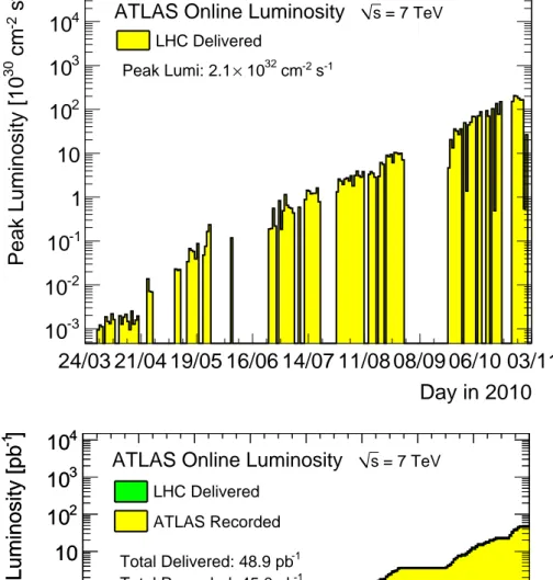
dtL is the integrated luminosity. Figure1.2shows how the
instanta-neous and integrated luminosity have increased in the period March-November 2010. The
delivered luminosity in 2010 is of about 40 pb−1, and at the end of 2011, the luminosity
Day in 2010
24/03 21/04 19/05 16/06 14/07 11/08 08/09 06/10 03/11
]
-1s
-2cm
30Peak Luminosity [10
-310
-210
-110
1
10
210
310
410
ATLAS Online Luminosity
s = 7 TeV LHC Delivered -1 s -2 cm 32 10 × Peak Lumi: 2.1Day in 2010
24/03 21/04 19/05 16/06 14/07 11/08 08/09 06/10 03/11
]
-1Total Integrated Luminosity [pb
-5
10
-410
-310
-210
-110
1
10
210
310
410
Day in 2010
24/03 21/04 19/05 16/06 14/07 11/08 08/09 06/10 03/11
]
-1Total Integrated Luminosity [pb
-5
10
-410
-310
-210
-110
1
10
210
310
410
= 7 TeV sATLAS Online Luminosity
LHC Delivered ATLAS Recorded -1 Total Delivered: 48.9 pb -1 Total Recorded: 45.0 pb
Figure 1.2: (Top) Development of the LHC peak luminosity in 2010. (Bottom) Integrated luminosity in 2010 delivered to (green) and recorded by ATLAS (yellow) during stable beams and for pp collisions at 7 TeV centre-of-mass energy.
Figure 1.3: Scheme of the ATLAS detector.
1.2
The ATLAS detector
The ATLAS Collaboration is an international collaboration, spanning the whole globe. It was born in 1992 by merging two proto-collaborations, and the detector concept was basically settled by the time of the preparation of the ATLAS Technical Proposal in 1994. The ATLAS detector was designed to cover the widest possible range of physics studies, from the search for the Higgs boson to supersymmetry (SUSY) and extra dimensions. The detector is designed for the study of high energy proton-proton and ion-ion high energy collisions. Of particular interest for the physics at LHC are the collisions that produce energetic particles emerging roughly perpendicular to the axis of colliding beams, the so
called high transverse momentum (high-pT) phenomena.
To cover a wide range of physics, the ATLAS detector was designed with a cylindrical layout, and with a forward-backward symmetry with respect to the interaction point. A precision tracking system (Inner Detector) surrounds the interaction region, operating in a solenoidal magnetic field. The inner detector is surrounded by a system of calorimeters, followed by a muon tracking system with a dedicated toroidal magnetic field. The funda-mental choice of two separate magnetic systems, one for the internal tracking, and one for the outer muon tracker, has driven the design of the rest of the detector. The present layout has been designed to fulfill the following requirements:
• very good electromagnetic calorimetry for electron and photon identification and measurement, complemented by full-coverage hadronic calorimetry for accurate jet
and missing transverse energy (ETmiss) measurement;
ac-curacy at the highest luminosity using the external muon spectrometer alone;
• efficient tracking at high luminosity for high-pT lepton momentum measurement,
electron and photon identification, tau lepton and heavy flavor identification, and full-event reconstruction capability at lower luminosity;
• triggering and measurement of particles at low-pT threshold, providing high
effi-ciency for most physics processes of interest at the LHC;
• fast and radiation hard detectors due to the experimental conditions at the LHC, and high detector granularity to handle the particle fluxes and to reduce the influence of overlapping events.
The next sections describe the subsystems of the ATLAS detector, with more emphasis on the most relevant systems used to measure the inclusive jet cross section. A general and detailed description of the ATLAS detector, and of its performances is provided in
Refer-ences [ATLAS Collaboration 2008a,ATLAS Collaboration 2009b]. As an introduction to
the geometrical coordinates used in this Chapter, the ATLAS reference system is described in the following lines.
Coordinate system in ATLAS
ATLAS uses a right-handed coordinate system with its origin at the nominal interaction point in the center of the detector. The z-axis is defined along the beam pipe direction, which defines the longitudinal direction, and the transverse (x, y)-plane as the plane per-pendicular to the beam direction. The x-axis points from the interaction point to the center of the LHC ring, and the y-axis points upward. For the transverse plane, the cylindrical coordinates (r, φ ) are used. The azimuthal angle φ is the azimuthal angle around the beam pipe, referred to the x-axis. The angle with respect to the beam pipe, θ is used to define the pseudo-rapidity η = − log tan θ /2. Zero pseudo-rapidity corresponds to the plane per-pendicular to the beam-line through the interaction point. Closer to the beam axis, the pseudo-rapidity grows towards positive (negative) infinity. The pseudo-rapidity is a geo-metrical quantity which corresponds, in the limit of 0 mass particles, to the rapidity, defined
as y = 1/2 log (E + pz)/(E − pz). The rapidity y (and as a consequence the pseudo-rapidity
η ) is an important variable in hadronic colliders. The center of mass frame of the hard scat-tering can have a longitudinal boost with respect to the laboratory. The difference of two rapidities (∆y) is invariant under longitudinal boost, making the rapidity an important vari-able in hadron colliders, and making the pseudo-rapidity more suitvari-able than θ to describe the angles along the beam direction.
1.2.1 Inner Detector
The central tracking system in ATLAS, discussed in detail in
Ref-erences [ATLAS Collaboration 1997a, ATLAS Collaboration 1997b,
ATLAS Collaboration 2010m], is designed to measure the track and the momentum of the charged particles produced in the collisions. To achieve the momentum and vertex
resolution, in the very large track density, high precision measurement must be made with fine detector granularity. The detector has been designed to be able to make high quality measurement assuming approximately 1000 particles emerging from the collision every 25 ns within |η| < 2.5 for the designed energy and luminosity. By measuring the positions of the hits of the charged particles with different radial layers of detectors, it is possible to reconstruct the direction of the outgoing particle, and through the curvature due to the magnetic field, the momentum of the track. The central tracking detector in ATLAS consists of three different technologies: the internal pixel detector, the silicon micro-strip semiconductor tracker (SCT) and the transition radiation tracker (TRT) surrounded by a super conducting solenoid providing a 2 T magnetic field. The inner detector has a cylindrical geometry, with a radius R=1.15 m and a longitudinal length of 6.20 m.
The strategy is to combine few high precision measurements close to the interaction point with a large number of lower precision measurements in the outer layer.
• Pixels: the pixel system consists of three concentric layers of semi-conductive pixels in the central region, and eight wheels in the region |η| > 1.7. A track typically hits three layers of Pixel, which measure both the r - φ and the z coordinates.
• SCT: the SCT consists of four layers of semi-conductive strips in the central region. In the end-cap they are arranged in wheels. A track typically hits four layers of SCT, which precisely measure the r - φ coordinate, and coarsely the z coordinate.
• TRT: the TRT provides a large number of hits (36). It consist of straw tubes parallel arranged to the beam axis in the barrel region, and in wheels in the end-cap. It only provides information in the azimuthal direction. The reduced resolution with respect to the inner detectors is compensated by the higher radius, and by the number of measured points.
The combination of precision trackers at small radii, with the TRT at larger radii, gives a very robust and precise measurement of tracks in all the detection directions. The internal semiconductor trackers also measure the part of the tracks closest to the interaction point, allowing the reconstruction of the possible primary and secondary vertexes, as introduced in the following lines.
Figure1.4shows two schematic views of the inner detector, with the geometrical
posi-tion of the different technologies. Vertexes
The analysis of the inclusive jet cross section uses the knowledge of the position of the primary interaction point, (primary vertex) of the proton-proton collision. The reconstruc-tion of the interacreconstruc-tion vertex is based on the reconstrucreconstruc-tion of charged particle tracks in the ATLAS inner detector. It is divided in two steps: (a) the primary vertex finding al-gorithm, dedicated to associate reconstructed tracks to the vertex candidate, (b) the vertex fitting algorithm, dedicated to reconstruct the vertex position and its corresponding error matrix. The measurement of the position of the primary vertex has a resolution of about
position of the vertex depends of the accelerator conditions. It can cause a shift of 0.5 mm in the transverse plane, and fluctuations of about 30-50 mm in the longitudinal direction. For this reason, during physics runs the luminous region (named beam spot) is determined by using the distribution of the recorded primary vertexes typically every 10 minutes. A detail description of the vertex reconstruction performances can be found in References [ATLAS Collaboration 2010b,ATLAS Collaboration 2010i].
The analysis of the inclusive jet cross section used the information of the primary vertex for two porposes: (a) to reject the non-collision background contribution, such as those due to the cosmic rays, by selecting events with at least one primary vertex; (b) to monitor the number of primary vertexes in the events, to properly correct for the particles produced by the additional proton-proton interactions per bunch crossing.
1.2.2 Calorimetric system
The calorimetric system selected for the ATLAS experiment consists of different technolo-gies, adopted to obtain the best performance in each geometrical region while maintaining a sufficient radiation resistance. The calorimetric system covers a wide range in pseudo-rapidity (η <4.9), and is completely hermetic in φ . This allows to obtain an accurate measurement of the jets in a large phase-space, and a good measurement of the missing transverse energy.
Given the difference in the shower development for electrons/photons and
hadrons, the calorimetric system is divided into two different sections: the
elec-tromagnetic section (EM), described in References [ATLAS Collaboration 1996a,
ATLAS Collaboration 2010j], and the hadronic section (HAD) described in References [ATLAS Collaboration 1996b, ATLAS Collaboration 2010k]. The EM section must pro-vide a good measurement and containment of the electromagnetic showers. The hadronic shower are instead measured by the ensemble of the EM and HAD sections that together contain at best the whole shower and limit the punch-through (i.e. particles leaking out of the calorimeter).
Thicker calorimeters improve the containment of the showers, however this has to be balanced against the increased material and dimension of the device. The two parameters which describe the thickness of a calorimeter, for the electromagnetic showers, and for the
hadronic showers, are the radiation length X0and the interaction length λI. The first one is
both (a) the mean distance over which a high-energy electron loses all but 1/e of its energy by bremsstrahlung, and (b) 7/9 of the mean free path for pair production by a high-energy photon. The second one is the mean distance traveled by a hadron before undergoing an
inelastic nuclear interaction. The total thickness of the EM calorimeter is more than 22 X0,
and for the containment of the hadronic shower, the calorimetric system has a thickness of
9.7 λI.
To achieve the required performance in a widely varying radiation environment the ATLAS calorimetric system uses radiation-hard liquid Argon (LAr) technology for the EM barrel and end-cap, for the hadronic end-cap (HEC), for the forward calorimeter (FCal). In the barrel region, the cryostat is shared with the super conducting solenoid, while the EM end-cap, the HEC and the FCal share the same cryostat in the forward region. In the
Figure 1.5: Overall view of the ATLAS calorimetric system.
barrel region, the tile calorimeter (TileCal) provides a good solution to precisely measure the energy loss by hadrons, with a relatively cheap technology. Scintillating tiles are used as active material, while the passive material is steel. The TileCal is divided in a barrel
(|η| <1) and two extended barrels (0.8< |η| <1.7). Figure1.5 shows an overall view of
the ATLAS calorimetric system. The calorimeters are divided in different radial layers of cells, which allow us to follow the longitudinal development of the electromagnetic and hadronic showers produced by the impinging particles. The design parameters for
the different ATLAS calorimeters are shown in Table1.2. The division in cells coarsely
follows a projective geometry, in which the detector is divided by different region of fixed pseudo-rapidity.
1.2.2.1 The electromagnetic calorimeters
The electromagnetic calorimeter is divided into a barrel part (|η| <1.475) and two end-cap components (1.375< |η| <3.2). The barrel consists of two identical half-barrels separated at z=0 by a 6 mm gap between them. The two end-caps are divided in two coaxial wheels. The absorber consist of lead, with an accordion geometry, which provide a complete sym-metry in φ without azimuthal cracks. The active material is the liquid Argon. Charged particles that cross the liquid Argon produce by ionization a current which is measured in electrodes. The electrodes which collect the signals envelop the absorber.
The barrel is divided in three longitudinal samples. The first one (4.3 X0long) has a fine
segmentation in η, to precisely determine the pseudo-rapidity direction of the impinging
Table 1.2: Design parameters of the ATLAS calorimeter.
EM CALORIMETER (LAr) Barrel End-cap
Coverage |η| <1.475 1.375< |η| <3.2
Long. segmentation 3 samplings 3 samplings 1.5< |η| <2.5
2 samplings 2.5< |η| <3.2 Granularity (∆η × ∆φ ) Sampling 1 0.003 × 0.1 0.025 × 0.1 1.375< |η| <1.5 0.003 × 0.1 1.5< |η| <1.8 0.004 × 0.1 1.8< |η| <2.0 0.006 × 0.1 2.0< |η| <2.5 0.1 × 0.1 2.5< |η| <3.2 Sampling 2 0.025 × 0.025 0.025 × 0.025 1.375< |η| <2.5 0.1 × 0.1 2.5< |η| <3.2 Sampling 3 0.05 × 0.025 0.05 × 0.025 1.5< |η| <2.5
PRESAMPLER Barrel End-cap
Coverage |η| <1.52 1.5< |η| <1.8
Granularity (∆η × ∆φ ) 0.025 × 0.1 0.025 × 0.1
Hadronic Tile (TileCal) Barrel Extended Barrel
Coverage |η| <1.0 0.8< |η| <1.7
Long. Segmentation 3 sampling 3 sampling
Granularity (∆η × ∆φ )
Sampling 1 and 2 0.1 × 0.1 0.1 × 0.1
Sampling 1 and 2 0.2 × 0.1 0.2 × 0.1
Hadronic LAr (HEC) End-cap
Coverage 1.5< |η| <3.2
Long. Segmentation 4 sampling
Granularity (∆η × ∆φ ) 0.1 × 0.1 1.5< |η| <2.5
0.2 × 0.2 2.5< |η| <3.2
FCal Forward
Coverage 3.1< |η| <4.9
Long. Segmentation 3 sampling
Figure 1.6: Overall view of the liquid argon calorimetric system.
of the energy loss by electrons and photons. The third layer, with a coarser segmentation, is used to measure the energy loss in the last part of the longitudinal development of the electromagnetic showers.
Figure1.6shows an overview of the liquid argon calorimeters.
The signals generated in the different cells are shaped, amplified and digitized by the front-end electronics, located in the gap between the TileCal barrel and the TileCal ex-tended barrel. The shaped signals are sampled five times at a frequency of 40 MHz. The digitized samples are transmitted to the Read Out Drivers (RODs) that contains Digital Sig-nal Processors that reconstruct the amplitude and time of the origiSig-nal sigSig-nal using a linear
combination (Optimal Filter - OF) [Cleland 1992] of the samples si. The energy in each
channel is given by:
Ecell(MeV ) = F
5
∑
i=1
ai(si− P) (1.3)
where F is the conversion factor between ADC counts and MeV, P is the cell pedestal
and ai are the optimal filtering coefficients. The linearity of the EM calibration has been
verified with test-beam electrons in the range 10-350 GeV. The scale of the calorimeter has
1.2.2.2 Hadronic calorimeters
The hadronic calorimeters enclose the EM calorimeter. Together they measure the energy
deposition of the hadronic showers. Given the small thickness in terms of λI of the EM
calorimeter, the hadronic calorimeters are designed to give, to the complete calorimetric system, a good containment of the hadronic showers. Furthermore, they are designed to be hermetic in φ and to cover a wide range in pseudo-rapidity (|η| <4.9). These features allow the ATLAS experiment to perform an accurate measurement of the jets in a large phase-space, and a good measurement of the missing transverse energy.
There are three types of hadronic calorimeters in ATLAS: the tile calorimeter, the hadronic end-cap calorimeter and the forward calorimeter.
The tile calorimeter
The central part of the hadronic calorimeter, TileCal, differs from the rest of the ATLAS calorimetry because it does not use the LAr as active material. The calorimeter is made by steel absorbers and scintillating tiles within the iron structure. The structure is periodical in z, and the tiles are oriented perpendicular to the beam axis. The tiles are read out by two wave length shifting (WLS) fibers, one for each side. The WLS fibers are grouped to reach
the desired cells granularity, reported on Table1.2.
Their signals are read by photo-multipliers located on the radial periphery of the calorimeter. Each cell is read out by two photo-multipliers to obtain a double readout.
The TileCal is subdivided into one barrel region (|η| <1.0), and in two extended barrels (0.8< |η| <1.7, one on each side of the barrel). The gap between them provides space for the services for the inner detector and the front-end electronics of the EM calorimeter. Both the barrel and the two extended barrels are subdivided in 64 modules, one for each φ slice
(∆φ ∼ 0.1). It is segmented in depth in three layers, approximately 1.5, 4.1 and 1.8 λIthick
for the barrel, and 1.5, 2.6 and 3.3 λIfor the extended barrel.
The front-end electronics of one TileCal module is placed on its external edge. The pulse produced by the photo-multipliers are shaped, amplified and digitized at 40 MHz with fast ADCs that provide, for each signal, seven samples. The signal is than processed
using the optimal filtering technique [Fullana 2005] to obtain the signal amplitude and time.
In this case however for all the signals above a predefined threshold it is also possible to save the complete digitized information.
The hadronic end-cap
Each one of the two hadronic end-cap consists of two independent wheels which cover the pseudo-rapidity interval 1.5< |η| <3.2. Both wheels consist of an array of copper plates, with a thickness of 25 mm in the first wheel, and 50 mm in the second one. The active material is the liquid Argon, which generates the currents read out by the electrodes. The gap between the plates is split by three electrodes into four drift spaces. The central electrode is the read-out electrode, while the side ones are the HV carries. Each wheel is
The signals in the cells, are sent to the preamplifier boards located at the wheel periph-ery, and the energy is reconstructed with a dedicated optimal filtering procedure.
The forward calorimeter
The radiation hardness of the liquid Argon technology is particularly important for the
for-ward calorimeter (FCal, described in detail in Reference [ATLAS Collaboration 2008b]).
This sub-detector is in fact facing an high level of radiation. Its front face is about 4.7 m from the interaction point, and it is really close to the beam pipe. Its position is shown
in Figure 1.6. It provides clear benefits both in terms of uniformity of the calorimetry
coverage, and in terms of radiation background for the muon spectrometer in the forward direction.
The FCal consists of three longitudinal sections: the first one is made of copper, while the other two are made by tungsten. The liquid Argon is the active material, and the cur-rents produced by the ionization are collected in electrodes for the measurement of the energy deposition. The main difference between the forward calorimeter and the other liq-uid Argon calorimeters in ATLAS is the geometry adopted to collect the signals. In each section, the calorimeter is made by a metal matrix with regularly spaced longitudinal chan-nels filled with concentric rods and tubes. The rods are at positive high voltage, while the tubes and the matrix are grounded. Rods are grouped for the readout totaling about 3500 channels.
The signals from the electrodes define the energy measured in each cells, by using a peculiar optimal filtering algorithm.
1.2.3 The muon spectrometer
The muon spectrometer is based on the magnetic deflection of muon tracks in the large superconducting air-core toroid magnets. The magnet configuration provides a field mostly perpendicular to the muon trajectory, while minimizing the degradation of resolution due to multiple scattering because the muons travel mainly through the air.
The muon spectrometer has been instrumented to have the possibility to perform a precise standalone measurement of the muon momentum. A detailed description of the
muon spectrometer can be found in Reference [ATLAS Collaboration 1997c].
In the barrel region (|η| <1.0), the muon chambers are arranged in three cylindrical layers (sectors), while in the end-cap (1.4< |η| <2.7) they form three vertical walls. The transition region (1.0< |η| <1.4) is instrumented with four layers.
The azimuthal layout follows the magnet structure: there are 16 sectors. The large sectors lie between the coils, and they overlap with the small sectors placed next to the
coils. Figure 1.7shows an overall view of the geometry of the muon sectors, and of the
different technologies used to detect and measure the muons.
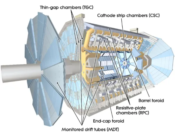
The choice of different types of chambers has been driven by criteria of rate capabil-ity, granularcapabil-ity, aging and radiation hardness. The measurement of the track bending is provided in most of the η regions by the Monitored Drift Tubes (MDT), while at large η , the higher granularity Cathode Strip Chambers (CSC) are used. The chambers for the
Figure 1.7: Overall view of the muon chamber system in ATLAS.
first level of the trigger system need a very fast response. They covers the region |η| <2.4. The Resistive Plate Chambers (RPC) are used in the barrel region, while the Thin Gap Chambers (TGC) are used in the end-cap.
The overall performance over the large area involved depends on the alignment of the muon chambers with respect to one another, and to the overall detector. The internal defor-mations and relative positions of the MDT chambers are monitored by precision-mounted alignment sensors. The magnetic field is continuously monitored, to be able to properly determine the bending power along the muon trajectory.
1.2.4 Trigger and Data acquisition
The ATLAS trigger and data-acquisition is based on three levels of on-line event
se-lection. Each trigger level refines the decision of the previous one. A detailed
de-scription of these systems can be found in References [ATLAS Collaboration 1998,
ATLAS Collaboration 2003]. Starting from an initial bunch crossing rate of 40 MHz, the rate of selected events must be reduced to about 100 Hz for permanent storage. The strong rejecting factor must match the need of an excellent efficiency for the rare physics pro-cesses of interest. The Level-1 trigger takes its decision based on a reduced granularity information from a subset of detectors. Objects searched by the calorimeter triggers are high transverse momentum electrons, photons, jets, hadronically decayed taus, as well as the missing transverse energy and the total transverse energy. The muons are identified
by the trigger chambers in the muon spectrometer. All the Level-1 trigger decisions are taken by logically combined requirements on these objects. No tracking information is used by the Level-1 trigger, due to the timing restrictions. The maximum rate at which the ATLAS front-end system can accept Level-1 triggers is limited to 70-80 kHz, but in the last year several tests to reach 100 kHz have been performed. Due to the geometrical size of the experiment (in some cases the time of flight to arrive to a sub detector is of the same order of magnitude of the bunch crossing period), and to the time in which the detec-tor signals extend, all the detecdetec-tor signals are sdetec-tored in pipelines. Events accepted by the Level-1 are read-out from these pipeline in the front-end electronics. The allowed Level-1 latency, measured from the proton-proton collision until the trigger decision is available to the front-end electronics, should be less than 25 µs.
All the detector data, selected by the Level-1 trigger, are collected from the different part of the detector to the Read Out System (ROS), until the event is processed by the High Level Trigger (HLT). The HLT consists of two different levels, the Level-2 and the Event Filter (EF).
The Level-2 trigger processors make use of the complete granularity information from the complete ATLAS detector. However, only data from a small geometrical portion of the detectors are used in the Level-2. These regions, called Regions of Interest (RoIs), are selected by the Level-1 trigger. The final Level-2 rate is expected to be about 1-2 kHz.
The Event Filter is the last step of the chain. It uses off-line algorithms, adapted for the on-line time requirements, to reconstruct the objects, and to take its decision. The Event Filter has about 1 second to take the decision, and the output rate is of about 100 Hz. The events selected by the Event Filter are written to mass storage for the subsequent off-line analysis.
In the next subsections, the relevant triggers used in the measurement of the inclusive jet cross section are presented.
Minimum bias trigger scintillators
The Minimum Bias Trigger Scintillators (MBTS) are 32 scintillator plates connected to different photo-multipliers. They are divided in two wheels, situated on the positive and negative LAr end-caps, covering the pseudo-rapidity range 2.1 < |η| < 3.8. For each wheel, there are 2 segments in η (inner and outer) and 8 segments in φ .
The MBTS were used to trigger on Minimum Bias events at early days running. Figure
1.8shows a picture of the position of the MBTS system.
The light produced in the scintillators is sent, via wave length shifting fibers to some of the TileCal multipliers. After an amplification step, the signals of the 32 photo-multipliers are sent to discriminators. If there is at least one signal above the discriminator threshold, the event is accepted by the Level-1 system. The name of the trigger which fires in this configuration is L1_MBTS_1, and it has been extensively used for the anal-ysis of the very first collisions, for the analanal-ysis of the minimum bias events and for the measurement of low transverse momentum jets.
Figure 1.8: Photo of MBTS mounted on LAr end-cap cryostat. MBTS is the gray annulus divided in 8 visible tiles. Fibers from MBTS go radially to photo-multipliers in TileCal. Jet triggers
The important units for the jet trigger algorithm are the jet RoIs and the Jet Windows. The energy in the electromagnetic and the energy in the hadronic calorimeters are summed in projective towers of ∆η × ∆φ =0.1 × 0.1. These towers are summed in RoIs to give a granularity of ∆η × ∆φ =0.4 × 0.4 (4 × 4 towers per jet element). They are used to indicate the position of the candidate jet.
The Jet Windows are windows of size 4 × 4, 6 × 6 and 8 × 8 projective towers, which slide in steps of two towers in both the η and φ directions. They are used to measure the
jet ET.
The requirements for the Level-1 single jet trigger are:
• The RoI cluster must be a local ET maximum compared to its neighbors;
• The jet window ET, for the granularity under consideration, must be greater than the
selected jet threshold.
Several sets of trigger ETthresholds are available in the ATLAS trigger menu. Each
thresh-old set is a combination of a threshthresh-old for jet ET (on which no hadronic calibration
proce-dure is applied) and a choice of jet window size.
In the first period of data taking the measurement of the inclusive jet cross section is based on events selected by the Level-1 jet trigger. In this period, in fact, the higher trigger levels were under commissioning and not used to reject the data. The list of the used trigger
Similar strategies are used to select the jets in the central region (up to |η| <3.2), by the central jet trigger and in the forward region (3.2< |η| <4.9), by the forward jet trigger. The measurement of jet in the region around 3.2 can be done using the OR combination of
the central and the forward jet trigger, as described in Section5.1.1.
The Level-2 jet trigger algorithm accesses calorimeter data that lies in a rectangular region centered around the Level-1 jet RoI position. The position and transverse energy of each detector element that falls into the chosen region are read-out by the algorithm. The elements are clustered in cone-shaped object in the (η, φ ) plane with a given radius
Rcone=
p
∆η2+ ∆φ2. The jet energy and position are found through an iterative algorithm,
which runs N times. In the first step the center of the jet is the position of the Level-1 jet
RoI (η0,φ0). In the i + 1 iteration the position of the cone (ηi+1,φi+1) is defined as the the
centroid of the cone opened around the center (ηi,φi) in the i iteration.
The requirements for the Level-2 single jet trigger is that at least one of the jets in the
event passes a threshold in ET.
The subsequent trigger selection is done by the Event Filter. This algorithm was un-der commissioning in 2010, and it was used in pass-through (even if the decision of the Event Filter was evaluated, it was not taken into account for the data acquisition). A de-tailed description of the algorithms used in the Event Filter can be found in Reference [ATLAS Collaboration 2009c].
1.2.5 Monte Carlo simulation of the ATLAS detector
The ATLAS sub-detectors have been exposed to beams in several test in the last 20 years. These tests were aimed at proofing the expected performances of the technolog-ical solutions adopted by the experiment, and to improve the Monte Carlo description
of the detector. The ATLAS detector simulation software [ATLAS Collaboration 2010n]
is based on GEANT4 [Agostinelli 2003], and it uses the GEANT4 physics list
QGSP_BERT [A.Ribon 2010]. The simulations have been widely used in the last years,
not only to check the performances of the detector, but also to develop techniques for the analysis of the data. Part of the ATLAS event reconstruction depends on the accuracy of the Monte Carlo description of the geometry and of the defects of the detector. The accu-racy of these descriptions have been studied with several dedicated analysis using the first proton-proton collisions.
1.2.6 The data samples collected in 2010
The quest for higher and higher luminosity has implied to work with continuously changing accelerator and detector conditions especially from the point of view of the trigger system. The data recorded in 2010 have been divided in various periods. Within each period the accelerator and the detector conditions can be considered uniform. The general description of the operation conditions and the integrated luminosity collected in each period are shown
in Table1.3. The list of data indicated in Table1.3has been used for the measurement of
the inclusive jet cross section. The analysis strategy is designed to take into account the peculiarities of the different periods, and a cross check of the data stability has been done
Table 1.3: 2010 data periods for proton-proton running
Period Description Integrated
luminosity (nb−1)
A Unsqueezed stable beam data (β∗=10 m): 0.4
typical beam spot width in x and y is 50-60 µm.
B First squeezed stable beams (β∗=2 m): 9.0
typical beam spot width in x and y is 30-40 µm.
C More bunches in the machine 9.5
D Bunches with 0.9 × 10¹¹p/bunch - β∗=3.5m
Pileup: 1.3 interactions per bunch crossing (was <0.15 before)
Larger z-vertex distribution. 320
E New trigger menu, 1118
with operation for the trigger commissioning
F 36 colliding bunches in ATLAS 1980
G Bunch trains with 150 ns spacing from LHC 9070
H 233 colliding bunches in ATLAS 9300
I 295 colliding bunches in ATLAS 23000
and presented in Section5.2.
Detector status at the end of 2010
The subsystems have a natural evolution, partially due to the natural aging of the sub-detectors, partially due to the different conditions in the accelerator. In 2010 the ATLAS collaboration was able to record high quality data from all the subsystems, with an high fraction of good channels. The approximate fraction of operating channels at the end of
2010, shown in Table1.4, is in general higher than 97 %.
The efficiency integrated (and weighted by the weekly luminosity) over this data taking period is 93.6%. The inefficiency accounts for the turn-on of the high voltage of the Pixel, SCT and some of the muon detectors (2.0%) and any inefficiencies due to dead-time or due to individual problems with a given sub-detector that prevented the ATLAS data taking to proceed (4.4%).
Table 1.4: ATLAS detector status at the end of 2010
Subdetector Number of channels Approximate
operational fraction
Pixels 80 M 97.3%
SCT Silicon Strips 6.3 M 99.2%
TRT Transition Radiation Tracker 350 k 97.1%
LAr EM Calorimeter 170 k 97.9%
Tile calorimeter 9800 96.8%
Hadronic endcap LAr calorimeter 5600 99.9%
Forward LAr calorimeter 3500 100%
LVL1 Calo trigger 7160 99.9%
LVL1 Muon RPC trigger 370 k 99.5%
LVL1 Muon TGC trigger 320 k 100%
MDT Muon Drift Tubes 350 k 99.5%
CSC Cathode Strip Chambers 31 k 98.5%
RPC Barrel Muon Chambers 370 k 97.0%
Jet production at hadron colliders:
Theoretical predictions
Contents
2.1 Fundamental interactions: the Standard Model . . . 27
2.2 The Strong interactions: the Quantum Chromo-Dynamics (QCD) . . . 30
2.2.1 Structure of pQCD predictions . . . 30
2.2.2 From the soft divergences to the jet algorithms . . . 33
2.2.3 Beyond the fixed order predictions: the parton shower and non per-turbative effects. . . 38
2.2.4 Different strategies to get a predictions . . . 41
2.3 Inclusive jet cross section: Theoretical prediction. . . 43
2.3.1 Fixed order pQCD . . . 44
2.3.2 Total theoretical uncertainties for the fixed order predictions . . . . 50
2.3.3 NLO Matrix Element + Parton Shower . . . 51
2.1
Fundamental interactions: the Standard Model
The experimental observations and the theoretical developments in the last century dras-tically changed the description of the deepest properties of the matter, and of its funda-mental constituents. The fundafunda-mental constituents of the matter are the particles, which interact via different forces: the electromagnetic force, the weak force, the strong force and the gravitational force. All the fundamental particles and their interactions (but the gravity) are described by the Standard Model theory of the fundamental interactions. A detailed introduction to the Standard Model of particle physics can be found in References [Aitchison 2003,Aitchison 2004]. The particles and the forces are described by relativistic quantum fields, developed by the fruitful unification of the classical fields, the quantum mechanic and the special relativity.
The particles are divided in quarks and leptons depending on their interactions. In the Standard Model description, the quarks can interact through electromagnetic, weak, and strong interactions, with the strong interactions being the dominant one. Six different flavors of quarks are foreseen by the model and have been experimentally found: down, up, strange, charm, bottom and top. The leptons include charged leptons and neutrinos. The charged leptons are the electron, muon and tau. The corresponding neutrinos are known
Figure 2.1: The elementary particles in the Standard Model.
as the electron neutrino, muon neutrino and tau neutrino. Charged leptons can interact electromagnetically and weakly. The neutrinos can only interact weakly. At each particle correspond an anti-particle with equal mass and opposite charge.
The six quarks and the six leptons can be split up into three generations of particles with similar properties, but with different masses. The three generations contain (d, u, e,
νe), (s, c, µ, νµ), and (b, t, τ, ντ). The "normal" matter is made of up quarks, down quarks
and electrons. The quarks are "glued" together by the gluons, to form the nucleons and the atomic nuclei, and the electron interact with the nuclei via electromagnetic interactions, carried by photons, to form atoms and molecules.
The second and third generation of quarks and charged leptons have a short lifetime. The general properties of the fundamental particles of the Standard Model are reported in
Figure2.1.
These particles in the Standard Model are described by relativistic quantum fields. The general structure of the quantum mechanics and of the special relativity forces the fields to be invariant under fundamental symmetries. The interactions between different fields
are introduced by requiring the invariance under an additional symmetry: the local gauge symmetry. The symmetry group that produces the interactions in the Standard Model is
U(1) × SU (2) × SU (3). The U (1) is a complex phase and SU (2) and SU (3) are unitary
matrices with determinant one and rank two and three respectively. The detailed description of this symmetry, and its implication on high energy interactions is beyond the scope of
this document, and can be found in References [Aitchison 2003, Aitchison 2004]. The
requirement of maintaining the gauge additional invariance introduces a specific set of dynamics.
The invariance under U (1) and SU (2) leads to the theory of the electroweak
interac-tions. Four particles mediate the electroweak interactions: the photon (γ), the W+, the
W−and the Z0. The photon is responsible for all the electromagnetic interactions and has
no mass. The other electroweak gauge particles are massive and are seen in much rarer processes.
The invariance under SU (3) is responsible for generating the strong interaction. The strong charge is called color and it can take three values (usually called red, green and blue) and their anti-values (anti-red, anti-green, anti-blue). The sum of the three colors is charge neutral. The strong interaction has one massless mediator, the gluon, which also carries color and anti-color charge. An important peculiarity of the strong interaction is that the force gets stronger at large distances. This has profound consequences. One of them is that strongly interacting particles can only be observed in color-neutral bound states (the hadrons). This property is known as confinement. Any attempt to separate a quark or gluon from its bound state results in the production of new color-neutral particles rather than a free quark or gluon. The protons and the neutrons are the "common" bound states of strongly interacting up and down quarks.
The final piece of the Standard Model is the Higgs particle. The Higgs particle is
the footprint of a mechanism which provides the masses to the W±, to the Z0 and to all
the fundamental particles within the Standard Model (including itself). So far the Higgs particle is only a postulate and has not been confirmed experimentally. One of the goal of the Large Hadron Collider experiments is to investigate the presence of the Higgs boson and its dynamics.
2.2
The Strong interactions: the Quantum Chromo-Dynamics
(QCD)
The Quantum Chromo-Dynamics (QCD) is produced by the invariance under the SU (3)
local gauge symmetry. It is the Standard Model description of the dynamics of the
strong interactions. A complete introduction to the QCD can be found in References [Dissertori 2010, Salam 2010]. This section is an introduction to some of the important aspects involved in the determination of the theoretical prediction for the inclusive jet cross section at the LHC.
There are different first-principles approaches to solve QCD. The most complete
ap-proach is lattice QCD [Gupta 1997]. It involves a discretization of the space-time. The
values of the quark and gluon fields are considered at all the vertices/edges of the result-ing 4-dimensional lattice. The method is fruitful to calculate static quantities, such as the hadron mass spectrum, but at present it is not suitable to carry out a complete lattice calcu-lations of the LHC physics.
The approach used in hadron colliders to describe the strong interactions is through the perturbative QCD (pQCD). In this approach, the important parameter is the coupling which determines the strength of the force. Perturbative QCD relies on the idea of an order-by-order expansion in a small coupling.
The couplings in the Standard Model have a dependence on energy or distance. For the electromagnetic and the weak force the coupling gets stronger as one goes to higher energies or shorter distances, while for the strong force the opposite is true. The coupling
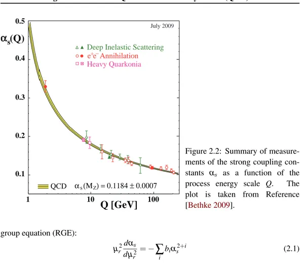
for the QCD is named αs and Figure 2.2 shows the decreasing of the strong coupling
constant αsas a function of the scale of the process, as obtained from the measurements in
several experiments (Reference [Bethke 2009]).
The strong force is weaker at small distances and high energies and gets stronger as the distance between particles increases. The fact that in QCD the force is weak at small distances is known as asymptotic freedom. The property of asymptotic freedom means that
in the high energy regime (Q& 5-10 GeV), physics can be described well by perturbation
theory.
Colliders like the LHC are mainly investigating phenomena involving high energy scales, in the range 50 GeV to 5 TeV. For these values the QCD coupling is small and the perturbation theory can be applied.
2.2.1 Structure of pQCD predictions
The strong coupling
In the framework of perturbative QCD, the predictions of observables are expressed in
powers of the renormalized coupling αs(µr2), a function of an (unphysical) renormalization
scale µr. Renormalization is a way to remove infinities from the theoretical predictions,
absorbing some terms in the coupling which acquires a scale dependence. The value of αs
is not calculable in perturbative QCD, but the value measured at a certain scale (usually
QCD α (Μ ) = 0.1184 ± 0.0007s Z 0.1 0.2 0.3 0.4 0.5
α
s(Q)
1 10 100Q [GeV]
Heavy Quarkonia e+e– AnnihilationDeep Inelastic Scattering
July 2009
Figure 2.2: Summary of measure-ments of the strong coupling
con-stants αs as a function of the
process energy scale Q. The
plot is taken from Reference [Bethke 2009].
group equation (RGE):
µr2dαs dµ2 r = −
∑
i biαs2+i (2.1)The coefficients bi, which determine the running of the coupling constant, can be calculated
in pQCD. When one takes µr close to the scale of the momentum transfer Q in a given
process, αs(µr2∼ Q) is indicative of the effective strength of the strong interaction in that
process.
The partons
Even if the high energy hadron colliders accelerate hadrons (i.e. protons), the fundamental interacting particles in pQCD are the quarks and the gluons (named partons).
In the cross sections involving initial state hadrons (such as in proton-proton collisions), a mapping between the kinematic properties of the initial hadrons to the initial partons is needed. This mapping is provided by the non-perturbative parton distribution functions
(PDFs). The PDF fi|h(x, µ2f) is the probability density of partons of type i inside a
fast-moving hadron h to carry a fraction x of the hadron longitudinal momentum. The scale µf is
the factorization scale. Its role is to handle the parton emissions which are collinear with the initial parton. The majority of the emissions that modify a parton’s momentum are actually collinear (parallel) to that parton, and do not depend on the fact that the parton is destined to interact in the hard process. It is natural to view these emissions as modifying the structure of the proton rather than being part of the hard partonic interaction. The separation between the two categories is somewhat arbitrary and parametrized by a factorization scale
] 2 [GeV 2 f µ 10 102 3 10 104 5 10 106 ) 2 f µ , x( i|p f × x -3 10 -2 10 -1 10 1 = 0.1 x up down up-bar down-bar strange charm bottom gluon HEPDATA Databases CT10 x -4 10 10-3 10-2 10-1 ) 2 f µ , x( i|p f × x -3 10 -2 10 -1 10 1 10 2 =[100 GeV] 2 f µ up down up-bar down-bar strange charm bottom gluon HEPDATA Databases CT10
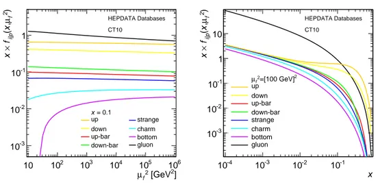
Figure 2.3: Dependence of the proton PDFs on the scale µ2f and on the
frac-tion of longitudinal momentum x, for the CT10 fit. Values extracted from Reference [http://durpdg.dur.ac.uk/].
fi|h(x, µ2f ∼ Q2) becomes indicative of the effective parton density function which enters in
the hard process.
The value of fi|h can be measured in different experiments (usually in deep
inelas-tic proton-electron scattering) and it can be evolved to other scales µf, thanks to the
Dokshitzer-Gribov-Lipatov-Altarelli-Parisi (DGLAP) equation, which at leading order is:
∂ fi|h(x, µ2f) dµ2f =
∑
j αs(µ2f) 2π Z 1 x dz z P (1) i← j(z) fj|h( x z, µ 2 f) (2.2)The coefficients Pi← j(1)(z) describe the probability for a parton j to emit a parton i which
carries a fraction z of his momentum. These coefficients, known as splitting functions, can
be calculated in pQCD. Figure2.3show the proton PDFs fi|p(x, µ2f), for the CT10 fits (see
Reference [Lai 2010]). The two plots show the dependence of the PDFs for the different
partons on the x and µ2f values.
pQCD predictions at hadron colliders
Once defined the strength of the strong force (αs) and how to evolve the hadron
(proton)-parton mapping for the initial state, one can calculate the cross section of a certain final state
X. The cross section factorizes in two terms: the probability of having a certain partonic
configuration in the initial state (i, j), and the partonic cross section ( ˆσi, j→X) that, given
the partonic initial state (i, j), describes the production of the final state X . This second
part can be expanded in power of αs : ˆσi, j→X = ∑∞n=0αsnσˆ
(n)
i, j→X. The master equation to calculate the pQCD cross sections in proton-proton colliders is:
σ ( p p → X ) = ∞
∑
n=0 αsn(µr2)∑
i, j Z dx1dx2fi/p(x1, µF2) fj/p(x2, µF2) ˆσ (n) i, j→X(x1, x2, µ 2 r, µ2f) (2.3)Figure 2.4:
Diagrams for
the 2 → 2 processes.
The diagrams are
divided in
differ-ent sub-processes
depending on the
initial and final state. This figure is taken
from Reference
[Ellis 1996].
Only the perturbative expansion of the partonic cross section is process dependent. The strong coupling constant and the PDFs are universal, and they can be measured in a wide variety of processes, in different experiments, and for different scales. The first non trivial
order in the perturbative expansion of ˆσi, j→X is named leading order (LO). The expansion
to the first two orders is named next to leading order (NLO). The perturbative expansion of the partonic cross section can (in principle) be calculated from first principles, but there are still many challenges that remain to be solved before we have a complete understanding of perturbative QCD.
2.2.2 From the soft divergences to the jet algorithms
The easiest QCD partonic processes are the 2 → 2 production: the scattering of two
incom-ing partons producincom-ing two outgoincom-ing partons. Figure2.4 shows some Feynman diagrams
for these QCD partonic processes. The leading order is proportional to αs2. It sums over all
the tree matrix elements |M22| with two incoming partons and two outgoing partons:
d ˆσ2(LO)= αs2|M22|dΦ2. (2.4)
where dΦ2is the phase space integration measure. By looking at the process 2 → 3, which
is the natural continuation after the 2 → 2, one can notice a general property of the pQCD calculations in the limit of collinear and soft emission. The first order in the perturbative
expansion is proportional to αs3:
d ˆσ3(LO)= αs3|M32|dΦ3 (2.5)
but if one of the final state gluon becomes collinear (parallel) to another particle i (the
inter-parton angle θig→ 0) and its energy tends to zero (it becomes "soft", Eg→ 0) the equation
2.5becomes: lim θig→0,Eg→0 d ˆσ3(0)∝ d ˆσ2(0)αs dθig2 θig2 dEg Eg (2.6)