Alma Mater Studiorum · Università di Bologna
Scuola di Scienze
Dipartimento di Fisica e Astronomia Corso di Laurea in Fisica
D
EVELOPMENT AND OPTIMIZATION OF THE
CONTROL SOFTWARE FOR A MOBILE
C
OMPUTED
T
OMOGRAPHY SYSTEM FOR
C
ULTURAL
H
ERITAGE
Relatore:
Presentata da:
Prof. Maria Pia Morigi
Simone Rossi Tisbeni
Correlatore:
Dott. Matteo Bettuzzi
Abstract
In quest’elaborato sono descritti l’ottimizzazione e lo sviluppo del software di controllo di un apparato tomografico con sorgente di raggi X per analisi nel campo di Beni Artistici e Culturali. In particolare, il lavoro è stato effettuato sul software preesistente di un sistema mobile in uso presso il Dipartimento di Fisica e Astronomia per indagini tomografiche. Il sistema, sviluppato nell’arco di più anni, consiste di un tubo a raggi X, un detector flat-panel e una tavola rotativa per la tomografia. Tre assi traslazionali consentono il movimento di detector e sorgente, ottenendo un'area scansionabile di 1,5×1,5 m². Il software di controllo si occupa dell’intero processo di acquisizione: gestisce il movimento degli assi, effettua la rotazione della tavola che sostiene l’oggetto durante la tomografia e controlla la scheda di acquisizione in comunicazione con il detector per la cattura delle immagini. Con l’upgrade sviluppato in questo lavoro vengono introdotte diverse routine automatizzate e una più comoda gestione delle regioni di interesse per la scansione radio-tomografica, con lo scopo di alleggerire il carico dell’operatore e ridurre i tempi di acquisizione. Il lavoro di tesi si conclude con un’indagine presso Palazzo Vecchio a Firenze in cui sono state effettuate analisi radiografiche e tomografiche di una serie di dipinti su tavola attribuiti in buona parte al Pontormo. In quest’occasione il software aggiornato è stato testato sul campo per verificarne la praticità e l’efficienza delle nuove funzioni. L’esperienza ha messo in evidenza alcuni problemi e carenze del software e del sistema stesso che suggeriscono l’opportunità di un certo numero di aggiornamenti e di una eventuale riscrittura del codice. Nonostante ciò, l’automatizzazione delle operazioni di acquisizione radiografica e tomografica si è rivelata efficace, riducendo il numero di interventi manuali richiesti e con essi il tempo necessario per l’analisi stessa.
i
Index
Introduction ... 1
Chapter 1. The X-ray radiation ... 3
1.1 Historical notes ... 3
1.2 Properties ... 4
1.2.1 X and Gamma rays... 5
1.3 Production ... 6
1.3.1 Spectrum of an X-ray tube ... 7
1.3.2 Beam hardening ... 9
1.4 Interaction with matter ... 10
1.4.1 Photoelectric absorption... 11
1.4.2 Compton scattering ... 12
1.4.3 Rayleigh scattering... 13
Chapter 2. The Tomographic technique ... 15
2.1 Radiographic principles ... 15
2.1.1 Good geometry and collimators ... 17
2.1.2 X-ray Detectors ... 17
2.2 Computed Axial Tomography ... 18
2.2.1 General considerations ... 19
2.2.2 Types of computed tomography systems ... 19
2.3 Reconstruction method ... 23
Chapter 3. CT system setup ... 27
3.1 X-rays source ... 27
3.2 Motion system ... 28
3.2.1 Translation axes ... 28
ii
3.3 Detector ... 31
3.4 Capture card ... 32
3.5 Control consoles... 33
3.5.1 Parrec ... 33
Chapter 4. The control software ... 35
4.1 State of the art ... 35
4.1.1 Image file format... 35
4.1.2 Image display window ... 36
4.1.3 Operating window ... 37
4.1.4 Translational axes controls ... 40
4.2 Shortcomings ... 41
4.3 Upgraded version ... 42
4.3.1 Standardization of the interface ... 43
4.3.2 New automated routines ... 44
Chapter 5. Field trial ... 49
5.1 System setup ... 49 5.1.1 Alignment process ... 51 5.2 Acquisition ... 52 5.2.1 Radiographic acquisitions ... 52 5.2.2 Tomographic acquisitions ... 53 5.3 Results ... 55 5.3.1 Future developments ... 56 Conclusion ... 57 Appendix ... 59 Appendix A ... 59 A1 - Control box ... 59 A2 - Capture card ... 60
iii
Appendix B ... 64
B1 - Axes movement function ... 64
B2 - Automated radiography ... 65
B3 - Automated tomography ... 66
1
Introduction
Computed Tomography (CT) is a powerful mean of investigation in the cultural heritage field, either for scientific investigation or for conservation and restoration purpose. This technique consists in the acquisition of multiple radiographic images at varying angle of the object to investigate, and the digital reconstruction of its sections. The application of this technique can give access to information on the invisible parts of a work of art, helping its restoration and conservation; often the tomographic reconstruction of an object can reveal hidden features, such as preparatory sketches, old restoration works, or even forgeries. Since this diagnostic technique is performed using X-ray radiation, it allows for a non-destructive way to inspect the inside of an artwork. In many cases, authorities do not permit to transport works of art outside of museums, so the development of a transportable X-ray CT system has become a necessity. In 2010, the X-ray Imaging group of the Department of Physics and Astronomy of the University of Bologna started developing a mobile ray imaging system, consisting of an X-ray tube and two motorized orthogonal axes translating an X-X-ray detector. In 2014, with the addition of a small rotating platform and later, in 2015, with the upgrade to new hardware and the addition of a vertical translation axis to move the X-ray tube, the system became a fully functional mobile CT scanner for on-site analysis [1].
This thesis works covers the latest upgrade to the system, in which the control software has been optimized to include semi-automated routines for the acquisition of radiographic and tomographic images. The main reasons that led to this development were the need to reduce the acquisition time and the number of manual intervention from the operator. Furthermore, by removing the need of a constant supervision during the acquisition process, the operator can simultaneously work on the reconstruction of the acquired images.
The work started in January 2016, during an internship at the Department of Physics and Astronomy, and run for the entire semester, during which the software was developed. Two different automated routines were implemented, one for the radiographic acquisition and one for the tomography. With the aim of increasing the versatility and usability of the system, optimized methods for the axes movement and the selection of the regions of interest were also added. After a series of lab tests to control the functionality of the software, the system was tried on-site for the first time at Palazzo Vecchio in Piazza della Signoria (Firenze) for an activity of radiographic and tomographic inspection of a series of wooden paintings by Jacopo da Pontormo [2].
2
These activities are presented in the five chapters of this dissertation.
The first chapter presents a brief introduction to the X-ray radiation with a summary of the main physical effects acting during its production and interaction with matter. The second chapter summarizes the different radiographic and tomographic techniques, with a brief mention to the algorithms used for the acquisition and reconstruction of the images, and a summary of the various generations of CT systems available.
The third chapter presents the components of the CT system developed by the X-ray Imaging group, with their characteristics and functionality.
The entirety of the fourth chapter is focused on the control software. In the first paragraphs, the state of the art is presented with an in-depth explanation of the software’s functionalities. The last paragraphs are dedicated to the upgrades developed to overcome the shortcomings of the previous version.
Finally, the fifth chapter presents the on-site experience at Palazzo Vecchio. The system setup is described and few examples of the acquired images are shown. The last paragraphs focus on the results of the tests, with limitations of the current version and potential future developments highlighted.
The appendices, in the last pages of this work, contain a summary of the libraries and APIs used to program the hardware, and some example of the code that has been written to develop the new routines.
3
Chapter 1.
The X-ray radiation
X-rays are a type of ionizing radiation that exhibit both wave-like and particle-like properties. The wavelengths of X-rays are so short that they can travel far through matter. For these reasons they are both useful, for inspecting the inside of an object, and dangerous, since the ionizing radiation can damage living tissue. In this chapter, the history and properties of x-ray radiation are briefly described, followed by a summary of the processes happening during their production and their interaction with matter.
1.1 Historical notes
The first published records on the X-ray radiation dates to December 28, 1895, when German physicist Wilhelm Röntgen submitted to the Wurzburg Physical-medical Society journal his paper "On a New Kind of Ray, A Preliminary Communication" few months after his discoveries. [3]
Figure 1.1. Hand mit Ringen (Hand with rings): print of Wilhelm Röntgen first “medical” X-rays
Like many other physicists of the time, Röntgen was working with diverse types of discharge tubes for cathode-ray emission, namely a Crooks tube such as the one used later by J.J Thomson to discover the electron. While studying the apparatus he noticed a faint glow light on a fluorescent screen placed some meters away from the tube. Apparently, some kind of invisible rays passed through the black cardboard he wrapped around the system to avoid interference from the visible light. Röntgen observed that the barium platinum-cyanide coated screen
4
acquired a black streak each time the tube was activated, even if placed at distances up to 6 meters, when either the coated or uncoated side of the paper faced the tube. This effect could not be caused by cathode-rays since those can travel in the air for at most a couple of centimeters. Further experiments revealed that this new kind of rays could penetrate many materials and the penetration power was dependent on the density of the substance they struck. He referred to this new kind of radiation as "X" due to its mysterious nature. The name stuck, even if in some languages (including German, Russian, and Japanese) they are still called Röntgen rays. [4]
Moreover, Röntgen discovered their medical uses when he made a radiographic picture of his wife's hand, the first picture of a human body part using X-rays (Figure 1.1).
His discoveries granted him the first Nobel Prize in Physics "in recognition of the extraordinary services he has rendered by the discovery of the remarkable rays subsequently named after him". [5]
1.2 Properties
The X-ray radiation is a form of electromagnetic radiation which, in quantum theory of electromagnetism, consist of photons: elementary particles behaving either as waves or particles. Photons are characterized by their wavelength 𝜆 and their energy 𝐸 which is quantized and is greater for higher frequencies 𝜈. These quantities are related by Planck’s equation:
𝐸 = ℎ𝜈 =ℎ𝑐
𝜆 (1)
where ℎ is the Planck’s constant, the quantum of action, that is central in quantum theory. The wave aspect of photons appears mainly at lower frequencies, while the particle aspect is predominant for higher frequencies [6].
5 1.2.1 X and Gamma rays
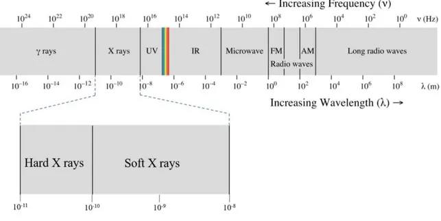
Figure 1.2. Complete spectrum of electromagnetic radiation with the X-ray portion highlighted.
X-ray radiation has a wavelength ranging from 0.01 𝑛𝑚 to 10 𝑛𝑚 with frequencies varying from 3 ⋅ 1016 𝐻𝑧 to 3 ⋅ 1019 𝐻𝑧 (Figure 1.2).
X-rays with low energies are called ‘Soft’ X-rays. Due to their low penetrating ability, they are easily absorbed in air.
Conversely, rays with high photon energy are usually called ‘Hard’ rays. Those are the X-ray photons used to image the inside of an object. Their high penetrating power, in fact, allows them to traverse relatively thick objects without scattering or being absorbed. The penetration depth varies over the X-ray spectrum allowing the photon energy to be adjusted for different applications whether in medicine, in research or in the industrial field [7].
Gamma ray photons cannot be distinguished from X-ray photons, thus, the distinction between the two types of radiation is based on their source: X-rays are emitted by the collision between a high energy electron beam and a metal, while gamma rays are produced during specific nuclear reaction (e.g. α or β decay and the capture of other particles) [6].
6
1.3 Production
Figure 1.3. Schematic depiction of an X-ray Tube. Electrons are emitted through thermionic process by the cathode C and accelerated toward the anode target A by a potential V. X-rays are emitted from the target upon impact.
X-rays are typically produced in an X-ray tube: a vacuum tube that uses a hot cathode to emit a beam of electrons accelerated through a potential difference of thousands of volts. The high velocity electrons are stopped upon striking a metal anode creating the X-rays, as shown in Figure 1.3. [8]
The electrons are usually produced from a tungsten filament, heated by a high electric current, in a process of thermionic emission. When the accelerated beam strikes the anode – usually tungsten, molybdenum or copper – only a small fraction of the kinetic energy of the electrons is transformed into X-rays; the remainder is subject to inelastic collision with the atoms and disperse its energy in the form of infrared radiation, heating the anode. To avoid degradation or even fusion of the anode, proper heat-control system are used, mainly liquid cooling circuits or rotating target; the latter allows the energy to be distributed on a larger surface because the beam collides on different points of the anode target.
The target is not perpendicular to the beam, but tilted in a way that the incident electrons interact with a bigger area, while the photons are emitted from an area effectively smaller called focal spot. Increases in the anode angle produce a bigger focal spot causing unsharpness in the image and resulting in a lower resolution. [6]
7 1.3.1 Spectrum of an X-ray tube
Figure 1.4. Radiation spectrum of a conventional X-ray tube. The continuous component, due to bremsstrahlung, and the discrete component due to characteristic emission are visible.
By measuring the intensity of the emitted X-ray photons as a function of their energy, we obtain the characteristic spectrum of a particular X-ray tube. The spectrum of the emitted rays depends on the applied potential difference, on the target’s material and, eventually, the presence of filters.
As shown in Figure 1.4, in the spectrum plot there are two components: a continuous one, due to Bremsstrahlung radiation, and a discrete one, due to characteristic emission of the atoms in the target.
Bremsstrahlung radiation
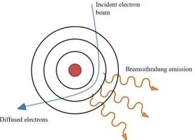
Also known as braking radiation, Bremsstrahlung radiation is an electromagnetic radiation produced by the X-ray tube with the deceleration of an electron from the beam when striking the target anode. The shape of the spectrum produced is a continuous curve that depends mainly on the energy of the incident electron beam and the accelerating potential V, while the minimum value of wavelength depends only on V. Studying the X-rays as emitted photons we can explain the elementary process in act as shown in Figure 1.5: when a free moving electron (originating from the beam) of initial kinetic energy Ki is decelerated by the interaction with a heavy nucleus (the target), the energy it loses gets radiated in the form of an X-ray photon. The electron interacts with the nucleus transferring momentum via the Coulomb field but, while the deceleration of the electron leads to the photon emission, the target is so massive that the energy it acquires can be neglected.
8
Figure 1.5. The Bremsstrahlung process responsible for the production of X-rays in the continuous spectrum.
With Kf the energy of the electron after the interaction, the energy (wavelength) of the emitted photon is:
hν = hc ⁄ λ = Ki− Kf (2)
The minimum wavelength represents the complete conversion of the electron’s kinetic energy in X radiation. Here Kf = 0 and Ki= eV the energy acquired by the electron moving through the accelerating potential V, we have
λmin = hc/eV (3)
Thus, explaining the wavelength cutoff dependent only on the potential difference. [8]
This process occurs not only in X-ray tubes but whenever there is a fast-moving electron interacting with matter.
9 Characteristic emission
Figure 1.6. Schematic representation of the characteristic emission process.
The discrete lines on the spectrum, superimposed on the continuum, are due to what is called characteristic emission. When traveling through the atoms of the anode an electron from the incident beam can interact with an electron in the inner subshell giving it enough energy, according to the Coulomb’s law, to remove it from its level and ejecting it from the atom. This results in a highly excited atom that will spontaneously return to its ground state by moving an electron from an upper level to the now incomplete state, thus emitting a high energy photon as represented in Figure 1.6.
The energy of the emitted photons is equals to the difference between the bound energy of the levels.
ℎ𝜈 = ℎ𝑐/𝜆 = 𝐸↑− 𝐸↓ (4)
The shape of the X-ray line spectrum is characteristic of the particular atoms composing the anode and provides information about the energies of the electrons in the inner subshells of the atoms. [8]
1.3.2 Beam hardening
The shape of the spectrum can be adjusted using a proper filter. The filtration is useful to remove the lower energy part of the X-ray beam, not strong enough to penetrate the object to inspect and, especially in medical use, source of unnecessary dangerous radiation. It is usually done by placing a thin metal screen (e.g. copper, aluminum) in front of the tube. This method
10
is called beam hardening, because it is used to reduce the emission of soft X-rays (lower energy) which are more easily absorbed than the harder ones. [6]
1.4 Interaction with matter
X-ray photons are energetic enough to free electrons from atoms and molecules, ionizing them and disrupting bonds. There are different interactions that cause this process: photoelectric absorption, Compton scattering, pair production, Rayleigh scattering and the photonuclear reaction. The probability of each interaction depends on the atomic number of the incident nuclei, the photons’ energy and the nature of the target material.
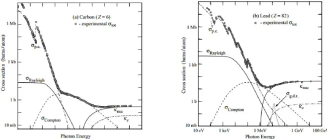
Figure 1.7. Photon cross sections for Rayleigh and Compton scattering, photoelectric absorption, pair production and photonuclear reaction for Carbon (a) and Lead (b) targets.
A measure of the probability of interaction, characterizing the collisions between photons and the target object, is given by the cross section 𝜎; The larger is the quantity, the higher is the probability of interaction. The total or cumulative cross section 𝜎𝑡𝑜𝑡 is the sum of all the cross sections of the interactions mentioned above. Figure 1.7 shows a plot of this quantity with the different interaction highlighted where:
- 𝜎𝑝.𝑒. is the cross section relative to the photoelectric effect; - 𝜎𝑅𝑎𝑦𝑙𝑒𝑖𝑔ℎ is the cross section relative to the Rayleigh scattering; - 𝜎𝐶𝑜𝑚𝑝𝑡𝑜𝑛 is the cross section relative to the Compton scattering; - 𝜎𝑔.𝑑.𝑟. is the cross section relative to the photonuclear reaction;
- 𝜅𝑛𝑢𝑐 and 𝜅𝑒 are the cross section relative to the pair production (for the interaction with nuclei and electrons respectively).
11
The photon energies used in radiography and tomography are low enough to neglect the effects of photonuclear reaction and pair production, more relevant in gamma radiation studies [9]. 1.4.1 Photoelectric absorption
Figure 1.8. Schematic representation of the photoelectric absorption.
In the photoelectric effect, a photon with low energy gets absorbed in the interaction with an atomic electron, which subsequently ejects from the inner subshell of the atom (Figure 1.8). The energy liberated in this ionization is the difference between the photon energy and the binding energy of the electron.
𝐸𝑒− = ℎ𝜈 − 𝐸𝑏 (5)
𝐸𝑏 is the minimum energy necessary for the interaction to happen.
Photon interaction cross section depends strongly on the atomic number of the absorbing material:
𝜎𝑝.𝑒. ∝ 𝑍4(ℎ𝜈)−3.5 (6)
The effect happens more frequently for higher bound state in the innermost shell when the photon energy is enough to rip the electron from the atom. This causes discontinuities in the cross section plot, in correspondence with the threshold energies. These discontinuities are more relevant for atoms with higher Z since the excited atoms can emit characteristic X-rays when returning to its ground state.
12
In general, the photoelectric effect makes the most contribution for energies lower than ~50 𝑘𝑒𝑉 for lighter atoms and energies lower than ~0.5 𝑀𝑒𝑉 for heavier ones [8].
1.4.2 Compton scattering
The Compton effect consist in the inelastic collision between a photon and an electron belonging to an outer shell of the target atom. In the interaction, the photon diffuses in a different direction, giving part of its energy to the electron which gets ejected from the shell (Figure 1.9).
Figure 1.9. Schematic representation of the Compton scattering.
The process is also called incoherent scattering, since the photon interacts with a single electron instead of the entire atom: in the interaction, the electron can be considered free [6]. The energy of the photon after the collision is:
ℎ𝜈 = ℎ𝜈
1+𝛾(1−𝑐𝑜𝑠𝜃) (7)
where ℎ𝜈 is the initial energy of the photon, 𝛾 = ℎ𝜈/𝑚𝑐2, and 𝜃 is the scattering angle.
While the kinetic energy of the electron is:
𝐸𝑒− = ℎ𝜈 − ℎ𝜈 = ℎ𝜈 𝛾(1−𝑐𝑜𝑠𝜃)
1+𝛾(1−𝑐𝑜𝑠𝜃) (8)
With higher initial energies, the scattering angle is increasingly lower.
13
𝜎𝐶𝑜𝑚𝑝𝑡𝑜𝑛 ∝ 𝑍 (9)
This process has effect for energies that range between 50 𝑘𝑒𝑉 and 10 𝑀𝑒𝑉 . 1.4.3 Rayleigh scattering
Also called coherent diffusion, this interaction takes place when the energy of the X-rays is significantly lower than the binding energy of the atom’s electrons. In this process, a photon collides elastically with the whole atom of the target material.
This causes a small deviation of the incident photon without any energy transferred to the atom, as shown in Figure 1.10.
Figure 1.10. Schematic representation of the coherent diffusion.
The cross section is proportional to the atomic number, and it is higher for heavier atoms:
𝜎𝑅𝑎𝑦𝑙𝑒𝑖𝑔ℎ = 𝑍2.5(ℎ𝜈)−2 (10)
The Rayleigh scattering is neglectable for high energies, where the other effects are more relevant. [8]
15
Chapter 2.
The Tomographic technique
Computed Tomography (CT) consists in the acquisition of multiple radiographies at varying angle of the object to investigate, and the digital reconstruction of two-dimensional section of the object (slice). The slices obtained are then rendered in a tridimensional representation of the volume of object. In this chapter, we will present the main principles of the radiographic and tomographic techniques and we will briefly talk about the reconstruction methods.
2.1 Radiographic principles
The radiographic technique is the most used non-destructive tool to investigate the inside of an object with X-rays. A radiographic picture is a planar map showing in each point the amount of X-ray absorbed by the object they passed through, dependent on its density and composition. The X-rays crossing a homogeneous material with depth 𝑑𝑥 are partially absorbed by the object, in a process called attenuation. The fraction of interacting X-ray photons is:
𝑑𝑁
𝑁 = 𝜇 ⋅ 𝑑𝑥 (11)
where 𝜇 = 𝜌𝑁𝐴
𝐴𝑟 𝜎𝑡𝑜𝑡 is the linear attenuation coefficient, which describes the fraction of a beam
of X-rays that is absorbed or scattered per unit thickness of the target object (Figure 2.1). In this equation 𝑁𝐴 is the Avogadro constant, 𝐴𝑟 is the relative atomic mass and 𝜎𝑡𝑜𝑡 is the total cross section, as defined in paragraph 1.4.
Figure 2.1. Representation of the X-rays attenuation.
What remain of the primary beam after the attenuation is known as remnant beam, which is responsible of exposing a detector placed after the object to investigate.
16
The number of photons hitting the detector after the interaction is obtained by integrating the differential expression above. With 𝑁0 the number of incident photons, we have: 𝑁 = 𝑁0𝑒−𝜇𝑥 Or, in terms of intensity of the beam, we obtain what is known as Lambert-Beer’s law:
𝐼 = 𝐼0𝑒−𝜇𝑥 (12)
If the material is not homogeneous the intensity of the detected beam will have a spatial distribution dependent on the object itself:
𝐼(𝑥, 𝑦) = 𝐼0exp − ∫ 𝜇(𝑠)𝑑𝑠𝑎𝑏 (13)
Where s is the axis parallel to the X-ray path.
The processes that characterize the interaction between the X-rays and the investigated object are those described in paragraph 1.4.
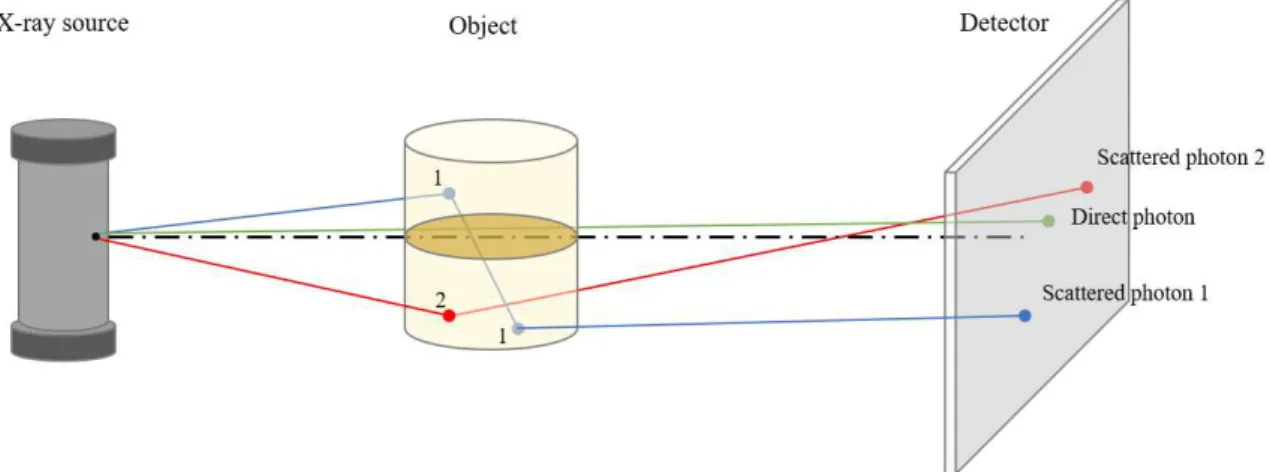
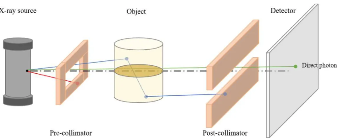
Figure 2.2. Schematic representation of an X-ray imaging system. Scattered and direct photons in the interaction with an object are shown.
For the range of energies relevant for radiography and tomography the only process that causes the absorption of the beam is the photoelectric effect. With that process part of the incident photons gets absorbed by the material, while the rest carries on the same trajectory and strike the detector. The Compton and Rayleigh scatterings, instead, cause some of the interacting photon to lose part of their energy and/or to get diffused on a different direction. This diffused radiation causes a loss of contrast in the image since it strikes the detector at a different angle, carrying no useful information, as shown in Figure 2.2
17 2.1.1 Good geometry and collimators
Figure 2.3. Pre-collimation and post-collimation of the radiation beam to reduce the scattered component.
The diffused radiation can be one order of magnitude larger than the direct radiation, a condition that is usually called bad geometry (Figure 2.2). To eliminate or reduce the scattered radiation, collimation devices – usually sheets of lead or other radio-opaque materials – can be placed in the path of the beam, bringing the system in a condition of good geometry (Figure 2.3). Depending on the type of detector (single, linear or planar), collimators can be placed before and/or after the object to inspect. [6]
2.1.2 X-ray Detectors
X-ray detectors are devices used to measure the spatial distribution of X-ray beams. They can be divided in two main categories: dose measurement devices (such as Geiger counter and dosimeters) and imaging detectors.
The formers are mainly used for safety purpose, measuring the radiation exposure, dose and dose rate, for verifying the effectiveness and security of radioprotection equipment and procedures; the latter are used investigate the inside of an object.
The first types of imaging detectors used where X-ray film, working similarly to photographic films: when exposed to radiation the silver halide grains on the film is ionized and the free electrons are trapped, forming a latent image.
This kind of detectors are now replaced by various digital devices, which can be subsequently divided in different families. A first distinction can be made on the method of acquisition: in direct acquisition detectors, the radiation forms an electric signal on the material of the detector proportional to the remnant beam’s intensity; in indirect acquisition, the radiation gets “converted” in visible light by a scintillator and read by a digital camera.
18
The main kinds of digital detectors used in high resolution radiography and tomography, are: - Charge Coupled Devices (CCD): constituted by a semiconductor, usually silicon, in
which the light produces pairs of electrons and vacancies. The higher the photon number, the higher the charge collected in a single pixel of the matrix that constitutes the detector. The image is obtained by measuring the charge collected in each pixel, and representing it in binary form.
- Flat Panel Detectors (FPD): either indirect or direct. The former presents a layer of scintillator (typically either gadolinium oxysulfide or cesium iodide) which produces the light that passes through to the subsequent layer: a thin film of transistors (TFT) in amorphous silicon. In each of the millions of pixels that form the detector there is a photodiode that produces an electric signal proportional to the light emitted by the scintillator layer. The signal is then amplified to produce the X-ray image. In direct FPD, the photons create electron-holes pairs in a layer of amorphous selenium that is read by a TFT array that converts it in binary form. [6]
2.2 Computed Axial Tomography
Figure 2.4. Conventional X-ray photography of a human chest.
Conventional radiography presents a fundamental limitation: the three-dimensional object to inspect is projected on a single two-dimensional plane, and the resulting image is composed by the superposition of the overlapping interior structure of the volume. Figure 1.4 shows an example of a chest X-ray study where the superposition of bones and organs is evident. Consequently, it suffers from poor contrast [10]. This limitation led to the development of the tomographic technique.
19 2.2.1 General considerations
The word tomography is derived from the Greek tomos meaning “slice, section” and graphos meaning “image, drawing” and is defined by the Oxford Dictionary as a “technique for displaying a representation of a cross section through a human body or other solid object using X-rays” [11]. This simple definition illustrates the main difference of this technique from conventional radiography.
Figure 2.4. Two projections, taken at right angle, of an object containing two cylinders, show as some details are not visible in one of them.
Let us consider a cylindrical object containing two smaller cylinders (Figure 2.4). By taking two radiographies from different angles we see a different content of the object depending on the projection angle. As shown in Figure 2.4, in the frontal projection the two cylinders are visible side by side, while in the left projection the smaller cylinder is covered by the larger one. To avoid this problem, computed tomography is based on a large number of different projections that are then used to reconstruct a complete section (or slice) of the inspected object [6].
2.2.2 Types of computed tomography systems
Image reconstruction from projections was attempted as early as 1940, without the aid of computer technology. A patent from those years by Gabriel Frank described a method very similar to modern days reconstruction, including drawings of equipment to form sinograms and backprojection techniques to reconstruct the image (this subject will be discussed in paragraph 2.3). In 1963 the first actual CT scanner was developed by nuclear physicist Allan
20
M. Cormack and, five years later, physiologist Godfrey N. Hounsfield built the first clinical tomography system. Because of their work both shared the 1979 Nobel prize in Physiology and Medicine [10]. The first laboratory equipment consisted of a low intensity gamma source, the scan was made by a linear beam on a rotating specimen in 1-degree steps. It took nine days to complete the acquisition and produce an image [10]. Today, thanks to
technological progress CT systems can produce a slice in less than 0.2s, thus enabling the display of a beating heart in real time [6]. Following their evolution through time, it is common to classify the distinct types of CT scanners in generations.
First-generation CT scanner
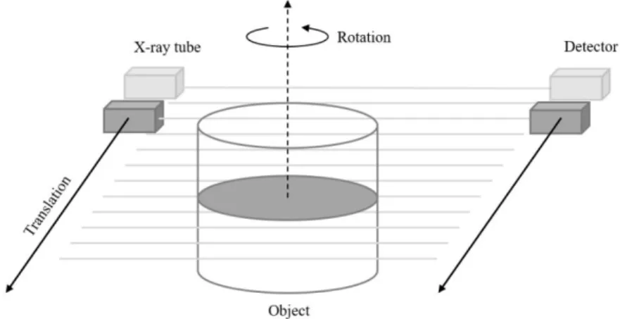
The first generation of CT systems are like the one adopted by Hounsfield in his experiments. This type of scanner is a translation-rotation system since the source is collimated to a narrow beam (pencil beam) that translates linearly along with the detector to acquire individual attenuation measurements and, after the movement is completed, the object is rotated to the next angular position and the process of acquisition starts over (Figure 2.5). Since the beams are parallel, a rotation of 180° total is sufficient. Where the object movement is difficult to achieve, as is the case for medical CT, the X-ray tube and detector are rotated instead [10].
Figure 2.5. First-generation of tomography system: a single detector scanning the object at each angle.
This type of sampling is called parallel projection. By translating the “source-detector” system and rotating the object by a small angular step it is possible to reconstruct a map of the linear attenuation coefficient, 𝜇(𝑥, 𝑦), in a slice of the object. Since the number of measurements cannot be infinite the resulting function is “pixelated”. The smaller the linear and angular step are, the better the resolution of the digital image will be. The proper mathematical procedure will be described in paragraph 2.3.
21
This type of system leads to the most accurate results in the image reconstruction but the process requires extremely long timeframes [6].
Second-generation CT scanner
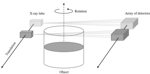
Figure 2.6. Second-generation tomography system: a linear array of detectors scanning the object at each angle with a lower step count.
In order to reduce the acquisition times, in the second-generation CT systems, instead of a single detector an array of multiple detector is placed opposite to the X-ray tube (Figure 2.6). This leads to a reduced number of steps, and subsequently a lower exposure time dependent to the number of detectors used. Unlike the first-generation scanners, though, the beams are not parallel and the acquisition must be then performed over 360º around the object. In medical CT, the patient is static and the “source-detector” system rotates around it. The number of angular steps decreases with the increase of the number of detectors in the array [10].
Third-generation CT scanner
Figure 2.7. Third-generation tomography system: a wide linear array of detector scanning the complete section of the object at different angles. The translation is no longer necessary.
22
The third-generation of CT scanners is the most widely used. In this configuration, many detector modules are arranged in a wide array opposite to the X-ray source (Figure 2.7). The system is stationary, since translation is no longer necessary. The entire object is always on the field of view of the array and rotates by small steps after each acquisition. In medical CT, the object is usually static and the “source-detector” system rotates around the patient. When the translation in the direction perpendicular to the slice and the rotation are synchronized the process is called spiral CT. In modern spiral CT systems, the array of detectors forms a full ring around the patient and only the X-ray source rotates along the spiral [6].
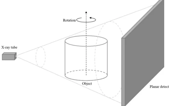
Cone-beam tomography
In this last generation of tomography systems, a full planar detector is used instead of a linear array. The image is produced from the source beam – in the shape of a cone – that irradiates the entire rotating object (Figure 2.8). This process – called Cone-Beam Computed Tomography (CBCT) – drastically reduces the acquisition time; the drawback is an increased percentage of diffused radiation, since no post-collimator can be used. If the detector is smaller than the projection of the object, macro-slices of the object are obtained by moving the detector (or the object) and later joined using dedicated software. Usually flat panels and CCDs coupled with a scintillating screen are used as viable planar detectors [6].
23
2.3 Reconstruction method
After the acquisition is done, the different projections are used to reconstruct the stack of cross sections (slices) of the investigated object. A single slice is a two-dimensional image of a specific internal section of the sample. As mentioned in the previous paragraph, since the number of measurements cannot be infinite, the image is composed by a matrix of elements called pixel. Following the same reasoning, each single slice should be considered as a section of the object with a non-zero thickness and the pixel matrix represents a grid of elements of volume called voxels.
Figure 2.9. Representations of the pixel matrix covering the object to inspect.
To obtain a mathematical description of the reconstruction let us consider a system with a parallel beam configuration crossing a single plane of the object and hitting a linear array of 𝑛 detectors (Figure 2.9.a). The slice of the investigated object can be divided in a grid of 𝑛 × 𝑛 pixels with attenuation coefficient 𝜇𝑖𝑗 and dimension 𝑤 × 𝑤, where 𝑤 is the size of a single module of the detector. The measures are repeated at different angles with fixed steps.
Assuming the incident beam is monoenergetic, the intensity measured by the detector is:
𝐼𝑗 = 𝐼0𝑒− 𝜇1𝑗+𝜇2𝑗+⋯+𝜇𝑛𝑗 𝑤 𝑗 = 1,2, … , 𝑛 (14)
pj= ln 𝐼𝑗
𝐼0 = ∑ 𝜇𝑖𝑗𝑤
𝑛
𝑖=1 (15)
The quantity 𝑝𝑗 is called projection and is the main measure on which the entire reconstruction process is based. When rotating the object (or the source-detector system), the beams are no longer aligned with the pixel matrix and the projection depends on the angle, with the photons
24
arriving on the detector after crossing a chord in the object that changes as shown in Figure 2.9.b.
In general, the projection is expressed as an integral of the two-dimensional function 𝑓 (𝑥, 𝑦) of the attenuation coefficient with parameters (𝜃, 𝑟) , where 𝜃 is the angle at which the projection is taken and 𝑟 is the distance of the projection ray to the center of rotation.
𝑥𝑐𝑜𝑠𝜃 + 𝑦𝑠𝑖𝑛𝜃 = 𝑟 (16)
𝑝(𝑟, 𝜃) = ∫ 𝑓 (𝑥, 𝑦)𝑑𝑠𝑟,𝜃 (17)
This last function is called Radon transform, from the name of the mathematician that first found the solution of 𝑓 (𝑥, 𝑦) from the line integrals. In this integral, 𝑠 is the axis parallel to the X-ray path.
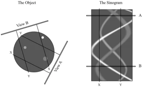
Figure 2.10. Schematic representation of the slice of an object and the corresponding sinogram.
To reconstruct a single slice, 𝑚 different acquisitions are needed at each 𝜃 angle consisting of 𝑛 projections. The matrix 𝑛 × 𝑚 obtained by the pixels of the different projections is called sinogram since the Radon transform of an off-center point source is a sinusoid, and the Radon transform of a section of the object appears as several blurred sine waves with different amplitudes and phases (Figure 2.10). The most commonly used algorithm for the reconstruction is called backprojection technique. This method takes the function obtained on each line of the sinogram and projects it back over the slice plane to produce the image. For each pixel, we have:
25
where 𝑓 ̂(𝑥, 𝑦) is the distribution of the attenuation coefficient obtained with this algorithm and Δ𝜃 is the angular step.
Considering the backprojection of a circular object, each profile projects on the plane a strip as wide as the object. Their superposition causes a star artifact (Figure 2.11). Increasing the number of projections this artifact produces a blur around the object that decreases in intensity with the distance from the center. To remove this effect a proper filter is applied on the projections and the resulting image (filtered back projection). The last two pictures in Figure 2.11 show the difference between the filtered and unfiltered projection.
Figure 2.11. Star artifact in a circular object’s backprojection. Filtered and unfiltered results are shown.
To obtain a 3D image of the object the various slices, acquired through the reconstruction process, are then stacked by means of a rendering software and the “dark” values filtered resulting in a tri-dimensional representation of the inspected object.
27
Chapter 3.
CT system setup
The applications of Computed Tomography are numerous, from the more common medical inspection to their use in analysis for cultural heritage. In this field, portable system for on-site analysis have become a real necessity since, in many cases, authorities do not allow to transport works of art outside museums. Therefore, a mobile X-ray CBCT system was developed and used successfully in multiple on-site works by the X-ray Imaging group of the Department of Physics and Astronomy of the University of Bologna [1].
This system is composed of 200 𝑘𝑉 X-ray tube, a 12 × 12 𝑐𝑚2 flat-panel detector and three
mechanical translation axes coupled with a rotating platform that provide a useful projection surface of 1.5 × 1.5 𝑚2. The operator controls all the components of the system thanks to a
control software on a remote connection computer placed at a safe distance [1].
In this chapter, the single components are presented and detailed. The last paragraphs are focused on the capture card and the software that is used for the control of the system and the reconstruction.
3.1 X-rays source
Figure 3.1. a) Picture of the X-ray Tube Smart EVO 200D. b) Picture of the control interface.
The X-ray tube used in the system is the Smart EVO 200D from YXLON international (Figure 3.1.a). The source is a high performance 750 𝑊 tube with a 1.0 𝑚𝑚 focal spot, air cooled, with a working temperature ranging from −20 º𝐶 to +50 º𝐶. The tube weights 23 𝑘𝑔, measuring
28
63.5 𝑐𝑚 in height and 29.5 𝑐𝑚 in diameter, making it ideal for a mobile system. The system operates at voltage ranging between 30 and 200 kV with electric currents ranging from 0.5 to 6.0 mA and can work on the highest configuration (200 𝑘𝑉 , 3.7 𝑚𝐴) for up to one hour of continuous exposure [12]. While this time is enough for radiography, it can be too short when acquiring a large number of tomographic images. This shortcoming will be further addressed in section 5.3.1. The tube comes with an interchangeable filter to reduce the lower energy emission and improve the image contrast. Full specifications of this model are presented in Table 3.1.
Table 3.1. Super EVO 200D X-ray tube specs [12].
Weight 23 kg
Height 635 mm
Focal spot size 1,0 mm High Voltage adjustment 30 – 200 kV mA adjustment 0,5 – 6,0 mA Max X-ray power 750 W Beam angle 40 º × 60 º Leakage radiation Max. 2.0 mSv/h
Environment IP65
Temperature range -20 ºC to +50 ºC Cont. Exposure 35 ºC, 200kV/3.7 mA 1 hour
The source is controlled from a safe distance with the compatible control interface shown in Figure 3.1.b.
3.2 Motion system
The motion system is composed of two axes for the detector movement, a vertical axis for the tube, a rotary platform for the inspected object and a rotary stage for the alignment of the detector.
3.2.1 Translation axes
The detector movement is managed by two perpendicular motorized axes, namely X-axis for the horizontal translation and Y-axis for the vertical one, both 1.5 𝑚 long. The two axes are separated for easier transport and can be assembled in order to obtain a wide area scanning device (Figure 3.2.a). The Y-axis is mounted on the translating platform of the horizontal one
29
and carries the detector. A third translation axis – named Z-axis – of proper size is used to carry the X-ray tube moving it vertically up and down (Figure 3.2.b). This axis is needed mainly for the tomographic acquisition where the source moves synchronously with the detector to keep the focal spot centered with the projection area [1].
Figure 3.2. Schematic representation of the translation axes: a) X-axis (horizontal) and Y-axis (vertical) carrying the detector; b) Z-axis for the X-ray tube movement.
The three axes are all controlled by a single control box to which they are linked by two different drive cables, one for the pair of perpendicular axes X Y, one for the Z-axis. The box is connected to the in-room computer through a serial port. In Appendix A1, the specifics of the communication parameters are explained (Table A.1).
The control box is fitted with manual controls for the axes movement and an emergency mushroom-head stop button (Figure 3.3).
Figure 3.3. a) Picture of the Control box for the translation axes. b) Schematic representation of the control box and its components.
30 3.2.2 Rotary stages
To achieve the rotation of the inspected object the rotary table PI-MICOS PRS-200 from Physik Instrumente is used (Figure 3.4.a). The table is a robust rotation stage, with a 160 𝑚𝑚 diameter, and capable of carrying a load of up to 50 𝑘𝑔 with a repeatability in the order of 1/1000 degrees [13]. This grants the reliability and precision needed for CT imaging. The table is placed on a tripod platform to increase the stability of the rotary table. The platform’s feet are adjustable in length to correct any possible slope of the floor and their adjustment allows a precise alignment of the system (Figure 3.4.b).
Figure 3.4. a) Picture of the PI-MICOS PRS 200 rotary table. b) Picture of the tripod platform with adjustable feet.
The rotatory axis is connected to the in-room computer through a USB port and managed by the control software.
An additional rotary stage is attached to the detector and its rotation allows the adjustment of the detector to ensure a correct alignment for radiographic and tomographic imaging. The stage used is a M-038.DG (Figure 3.5) from Physik Instrumente: a lightweight, high precision rotary stage with a 61 𝑚𝑚 diameter and a repeatability of 20 𝜇𝑟𝑎𝑑 [14].
31
The rotary axis is connected to the in-room computer through USB and piloted during the alignment stages of the acquisition process. After that, the stage is unplugged and remains unused until further adjustments are required.
3.3 Detector
The detector in use is a C10900D flat panel from Hamamatsu (Figure 3.6.b) coupled with a power supply from Christan Stapf Elektronik. The detector is mounted in a custom-made aluminum box with a radiotransparent window in front of the active area (Figure 3.6.a).
Figure 3.6. Pictures of the C10900D flat panel detector. With (a) and without (b) its custom box.
The FPD is an indirect panel with a layer of cesium iodide (CsI) scintillator directly deposited on the complementary metal-oxide semiconductor (CMOS) image sensor made up of a two-dimensional photodiode array where the electric charge is accumulated in each pixel according to the light intensity. The active area is approximately 12 × 12 𝑐𝑚2 with a pixel size
of 100 𝜇𝑚 and a pixel clock of 35.35 𝑀𝐻𝑧 [15].
The detector operates in 4 selectable scan modes: “Fast mode” and “Partial mode” with a pixel size of 200 × 200 𝜇𝑚2, or “Fine mode” and “Panoramic mode” with a pixel size of
100 × 100 𝜇𝑚2. The dimension of the active area changes depending on the selected mode as shown in Figure 3.7.
32
Figure 3.7. Active area for each scan mode of the detector.
Fine mode is useful for radiography and high-resolution tomography, with an image size of 1216 × 1232 pixels and a maximum frame rate of 17 𝑓𝑝𝑠. Fast mode, instead, allows faster acquisition at a lower resolution, ideal conditions for tomography of large sized objects. Timing and trigger mode
This FPD allows to use two different kind of triggers to time the acquisition. In internal trigger mode, the detector uses an internal frame grabber with fixed exposition time depending on the scan mode. In external trigger mode, the frame grabber of the capture card is used and it needs to be synchronized for sending to the detector the correct square wave for the selected scan mode. Although requiring a more accurate setup, with this configuration it is possible to adjust the exposition time (the frames acquired per second) allowing a fine-tuning of the resulting image contrast. For those interested in the specifics, more details on the different trigger methods can be found on the detector documentation [15].
3.4 Capture card
The capture card used is a PCI-1422 from National Instrument (Figure 3.8). This card acquires signals with frequencies up to 40 𝑀𝐻𝑧, compatible with the rates of acquisition of the detector. It features a programmable internal trigger and it supports resolutions of up to 16 bits, either in color or grayscale.
33
Figure 3.8. Picture of the PCI-1422 capture card.
The capture card settings are stored in a “ICD” text file that can be created with a National Instruments software called “Camera File Generator”. Eight different ICD files are created for the flat panel, one for each of the scan modes with the two different trigger settings. The capture card comes with NI-IMAQ: the libraries used to manage the acquisition process. An example of ICD file and a brief description of the libraries are presented in Appendix A2
3.5 Control consoles
The system is set up in the working room. The different axes are connected to an in-room computer through serial ports. The capture card is slotted in this computer and connected to the detector. The computer act as the control console of the system and runs the control software that manages the acquisition. This software manages the translational axes moving the detector and the source, and synchronizes the rotary stage movement with the capture card acquisition. A detailed explanation of the control software is presented in Chapter 4.
Since the working room is exposed to radiation during the acquisition, the user cannot stay inside to operate the console. Therefore, the computer is connected through an Ethernet port to a different PC in a room at safe distance (operator room). This setup allows the operator to work in a room unaffected by the radiations emission.
The computer in the operator room also runs the reconstruction software. 3.5.1 Parrec
The reconstruction software in use, named PARREC, was developed by Dr. Rosa Brancaccio at the Department of Physics and Astronomy of the University of Bologna. The software loads the sequence of projection files, with filename extension .sdt, and their respective .spr metadata
34
files. With the function named Makeatenrad the software normalizes the projections. It does so using the following formula, pixel by pixel:
𝐴𝑡𝑟𝑑𝑖,𝑗 = − ln 𝑃𝑟𝑗𝑖,𝑗−𝐷𝑟𝑘𝑖,𝑗
𝐼𝑍𝑒𝑟𝑜𝑖,𝑗−𝐷𝑟𝑘𝑖,𝑗 (19)
- 𝐴𝑡𝑟𝑑 is the resulting normalized projection; - 𝑃𝑟𝑗 is the original image acquired;
- 𝐷𝑟𝑘 is the Dark image, taken with the source of radiation shut down, corresponding to the signal generated by the thermal noise;
- 𝐼𝑍𝑒𝑟𝑜 is the image, taken without the object, that corresponds to the intensity of the beam when reaches directly the detector pixels.
The software then uses two different reconstruction algorithms: the first is a filtered back projection, in which the software, with a function called Makesinos, builds the sinograms corresponding to each slice and reconstructs them as explained in paragraph 2.3.
The second algorithm is the Feldkamp (FDK) algorithm that, conversely, reconstructs the object in vertical slices without building the sinograms of each slice.
These routines of the software are parallelized since the algorithms are very demanding in performance. Different filters are available to remove artifacts and errors.
The software is also used to merge different images, either radiographic or tomographic, through a collate function.
35
Chapter 4.
The control software
4.1 State of the art
The control software is developed in Lab Windows CVI: the SDK from National Instruments for the development of C/C++ software. The program was developed for the tomography system by R. Brancaccio, M. Bettuzzi, L. Ragazzini and A. Gallo and manages the communication between the flat panel and the capture card, and the movement of the rotary table. A subsequent upgrade added support for the translation axes of the detector (X and Y) and a routine for the acquisition of multiple adjacent radiographic images.
When the software is started the main screen is presented as shown in Figure 4.1.
Figure 4.1. The main window of the control software. The Commons tab is shown. The bottom part is dedicated to the translational axes controls.
The interface is divided in two separate windows: the first is the operating window containing the control and configuration tools; the second – named Image display window – is dedicated to the visualization of the acquired or loaded images (Figure 4.2).
4.1.1 Image file format
The projections that are acquired through the software are saved in a raw bitmap file with “.sdt” (signal data) filename extension. A raw bitmap is a generic image file that contains unprocessed data from an image sensor in the form of a map of the pixel “color” values. The
36
.sdt file contains the grayscale value of each pixel of the acquired image in a long array of raw bit data. Since a raw file does not contain any information on the dimension or bit-size of the image, an appropriate text file of the metadata is attached to the .sdt. This file is saved with the same name of the raw one with a “.spr” (signal parameters) extension.
An example of .spr file is shown in Table 4.1.
Table 4.1. Sample of a .spr file.
2 1216 0.000000 0.000000 1232 0.000000 0.000000 1
Dimensions of the array. 2 corresponds to a two-dimensional image. Number of columns Unused float Unused float Number of rows Unused float Unused float
Data type (1: Unsigned Short, 2: Unused, 3: Floating point)
4.1.2 Image display window
The Image display window shows the last image acquired or, eventually, a loaded image. The image is shown in full size and can be fitted to the size of the display window.
37
A tool windows can be opened to read information about the coordinates and grayscale value of the pixel hovered on by the mouse pointer. The available tools allow to control the zoom level, pan across the window and draw Regions of Interest (ROI) on the image.
A second support window is dedicated to the visualization of a histogram plot of the pixel value of the entire image or a selected ROI. A specific range of the histogram can be selected, either by clicking on the plot or by inputting the exact values. The window shows the statistic of the selected range: maximum and minimum values, mean value and standard deviation.
Both of those windows are visible in Figure 4.2. 4.1.3 Operating window
The operating windows is divided in multiple areas. A tab control window with multiple pages and its dedicated Log box, and an axes control window with its dedicated Log box. Both Log boxes show Debug messages and specific information on the running processes.
The tab control gives access to four different pages (or Tabs): Commons, Flat panel, Tomo, Hardware test. Through the menu strip a different image can be loaded (.sdt) and the image shown in the Image Display Window can be saved in different formats. The menu gives access to the settings window.
The bottom half of the window, instead, contains the translational axes controls and a routine for a large sample radiography (Figure 4.1).
Commons Tab
The commons tab gives access to quick acquisition functions, either a single image acquisition (Snap) or a continuous acquisition (Grab) with the possibility to set the number of frames being acquired and averaged. Three buttons are dedicated to the Image Display Window tools described in section 4.1.2. Through two radio buttons the image data type can be selected and switched between unsigned short or signed short. Lastly, the tab gives access to the rotary table controls (Figure 4.1). These processes are useful to check the proper functioning of the FPD and the axis at the start of the tomographic acquisition and they are necessary for the alignment procedures.
Flat panel Tab
The second tab, named “Flat Panel”, allows to switch between the eight acquisition modes described in section 3.3: fine, panoramic, fast and partial and either with internal or external trigger.
38
Figure 4.3. The Flat Panel Tab of the operating window.
Selecting one of these scan modes changes the ICD file loaded by the capture card. It is also possible to set the frame rate and exposure time in case of external trigger acquisition (Figure 4.3).
Tomo Tab
The third tab is dedicated to the tomographic acquisition and its parameters. The tab is shown in Figure 4.4.
Figure 4.4. The Tomo Tab of the control software.
The first field allows the selection of the work folder where the projection will be saved. The second text box changes the name of the saved files. The check box allows to switch between continuous or step by step acquisition.
In continuous acquisition, the rotary stage moves of the angle selected in the proper field. In this angle range the flat panel acquires continuously with the frame rate set in the Flat panel tab saving the projections in a Buffer list.
In step by step acquisition the number of projections taken in the angle range is selectable. The flat panel acquires the projections at regular steps using an average between a predetermined number of single frames, selected by the user through the dropdown list. The acquired projections can be then viewed and saved in the work directory, with the name chosen in the apposite field, followed by a number corresponding to their cardinality (i.e. “projection_0.sdt”,
39
“projection_1.sdt”, …, “projection_899.sdt”, …), as are their metadata files, that are saved in .spr format (i.e. “projection_0.spr”, “projection_1.spr”, …, “projection_899.spr”, …). The acquisition duration, in continuous mode, depends only on the rotary stage speed since the acquisition stops when the axis stops moving. On the contrary, in step by step mode, the duration depends on the number of selected projections. A timer shows the time left to the end of the acquisition process and the number of projections acquired in step by step mode. The last field, “Notes”, corresponds to a text file with the acquisition info and parameters; additional information can be added by the user.
This file is saved in the work folder with the projections. Hardware test Tab
Figure 4.5. The Hardware Test Tab of the operating window.
The fourth tab named “Hardware test”, contains the necessary function to test the flat panel connection (Figure 4.5). These commands are mainly used during development and debug and they are unessential during the acquisition.
Settings window
The settings window allows the selection of the default work directories and the path to the ICD file. On the bottom, there are the controls for the rotary stage: the connection parameters, the speed and the acceleration of the axis (Figure 4.6).
40
Figure 4.6. The settings window of the control software.
4.1.4 Translational axes controls
The bottom half of the operating windows is dedicated to the controls for the translational axis, with buttons for opening and closing the connection, resetting their position to the start and controlling their movement by setting the absolute coordinates of the X and Y axes (Figure 4.7).
Figure 4.7. The translational axes controls at the bottom of the operating window.
The commands that are used to control the axes are described in Appendix A1. Radiography routine
This section contains also the routine for the radiography of a wide area. Four number boxes allow the selection of the area boundaries in the X and Y coordinates (using integers from 0 to 15). The program moves the detector to the starting point and acquires the first radiography, it then moves to the second position with a step of 100 𝑚𝑚 in the X direction and acquires the second image. This process continues until the whole area is covered. If the selected area covers more than one Y position, the detector moves along the X axis until the end coordinate is
41
reached. It than moves to the next Y coordinate with a 100 𝑚𝑚 step and scans the next line in the opposite direction, as shown in Figure 4.8.
Figure 4.8. Schematic representation of the detector movement in the radiography routine. The arrows indicate the path of the detector.
The acquired radiographic images are saved in a .sdt file named “Radio_#_#.sdt”, where the two number signs are replaced with the Y and X coordinates (i.e. 0, 100, 200, …, 1500) respectively.
4.2 Shortcomings
The software, in its current state, allows the acquisition of both radiographic and tomographic images of objects of various size. Although, while the available functions are enough to manage the process, the software presents limitations and issues that slow down the acquisition and cause the need of several intervention by the user.
The control software was built to manage the tomographic acquisition of small objects, therefore, at first, it did not include support for the movement of the detector and the source. Since then, the software has been upgraded to include the controls for the translational axes but not all the routines were optimized and the controls were not properly integrated in the existing interface.
The axes controls do not include the Z axis of the source, that needs to be manually moved with the control box’s joystick.
42
The wide-area radiography routine works in steps of 100 𝑚𝑚 and cannot be adjusted differently. Furthermore, since the settable values for the X and Y ranges ends are integers between 0 and 15, the position of the detector is not very flexible. This can cause an increase in the number of radiographic images that needs to be acquired to cover the inspected object in its entirety.
The process also presents a bug when the detector is moved to a different line during the scan: at each iteration, the function sends to the axes a command with the absolute coordinates of the next position. When the detector needs to reach the next Y position a command is sent to the X axis with no difference in its absolute coordinate. This causes the axes to fail the movement and pointlessly attempt it until a 30 seconds timer expires.
Finally, the main shortcoming of this version of the software is the absence of an automatic procedure for tomographic acquisition. The system, as it is now, requires the intervention of the operator after each tomography to move the detector to the next position. For each subsequent position the user needs to change the working folder; failing to do so will cause the older projections to get overwritten. These shortcomings increase dramatically the working times.
The process also presents a bug when numerous successive tomographies are started: after a dozen of consecutive tomographies the program may try to reach a non-existing memory address and it fails to set the Buffer list. This causes the software to acquire void .sdt images without any warning. The only way to solve this issue is to restart the program, closing the connection with the axes. The operator therefore needs to enter the working zone to reset their position.
Every time the operator needs to enter the working zone, where the system is set up, the source must be turned off. After every restart, the X-ray tube takes up to a minute to reach the voltage and current set for the emission, causing further loss of time.
4.3 Upgraded version
With this thesis work, we tried to overcome these shortcomings, upgrading the control software. The work started in January 2016 with a curricular internship at the Department of Physics and Astronomy of the University of Bologna and ended with a case study in February 2017 at Palazzo Vecchio (Firenze).
The main objective was to automate the tomographic procedure and integrate the new routine in the previous version of the software.
43
The project, subsequently, evolved including fixes for most of the issues presented in the previous paragraph.
4.3.1 Standardization of the interface
The first notable upgrade is the adjustment made to the interface by including the axes control in the Commons tab. A new frame was added in the same format as the one for the rotary axis. The new tab is shown in Figure 4.9.
Figure 4.9. The Commons Tab in the updated version of the control software.
This section includes the controls for the translational axes communication and the function for the movement of the X, Y and Z axis. Each routine uses the same function, that is described in detail in Appendix B1. The program keeps in memory the last known position of the axes and it avoids sending a move command when no shift is needed. This precaution prevents the error with the translational axes movement that caused a 30 second delay as explained in paragraph 4.2.
The two separated log boxes have been unified into one and each function sends the debug messages to the same Log area.
The radiography routine of the previous version of the software has been kept for reference in this tab while, at the same time, being replaced with a new, more flexible, automated radiography routine introduced in the Tomo tab.
This upgrade in the interface reduces slightly the height of the operating windows, leaving more screen available for the Image Display window.
44 4.3.2 New automated routines
The main difference between the two versions of the software is visible in the Tomo tab (Figure 4.10).
Figure 4.10. The Tomo Tab in the updated version of the control software, with the new routines and specific regions selected.
The new interface includes two automated routines for radiography and tomography. Both routines use the same controls for the selection of the acquisition area, allowing a more precise control over the ROIs than the previous version. Another procedure allows to take a quick radiography of the entire area that can be covered by the detector. With this function, an image of the entire object is created and shown in the Image display window (Figure 4.11).
Figure 4.11. The Image display window. In the window, the full scan of a bicycle is visible. The regions highlighted corresponds to those selected in Figure 4.10.