Assimilation of data from conventional and non conventional networks through a LETKF scheme in the COSMO model

(1)

Alma Mater Studiorum

_{· Università di Bologna}

Scuola di Scienze

Corso di Laurea Magistrale in Fisica del Sistema Terra

Assimilation of data from conventional and

non conventional networks through a LETKF

scheme in the COSMO model

Relatore:

Prof. Rolando Rizzi

Correlatore:

Dott. Chiara Marsigli

Dott. Tiziana Paccagnella

Presentata da:

Mario Corbani

Sessione

III

(2)

(3)

Sommario

Il presente lavoro studia uno schema di assimilazione dati alla scala del km basato su un metodo LETKF sviluppato per il modello COSMO.

Lo scopo è di valutare l’impatto dell’assimilazione di due differenti tipi di dati: temper-atura, umidità, pressione e vento provenienti da reti convenzionali (SYNOP, TEMP, AIREP) e riflettività 3d da radar. Un ciclo di assimilazione continuo di 3 ore è stato implementato sul dominio italiano, costituito da 20 membri, con condizioni al contorno fornite dall’ensemble globale di ECMWF.

Sono stati eseguiti tre diversi esperimenti, in modo da valutare la bontà dell’assimilazione durante una settimana di ottobre 2014 caratterizzata dalle alluvioni di Genova e Parma: un primo esperimento di controllo del ciclo di assimilazione, con l’utilizzo di dati solo da reti convenzionali, un secondo esperimento in cui lo schema SPPT viene attivato nel modello COSMO, un terzo esperimento in cui è stata assimilata anche la riflettività proveniente da radar meteorologici.

È stata poi effettuata una valutazione oggettiva degli esperimenti sia su caso di studio che sull’intera settimana: controllo degli incrementi dell’analisi, calcolando la statis-tica di Desroziers per dati provenienti da SYNOP, TEMP, AIREP e radar, sul dominio italiano, verifica dell’analisi rispetto ai dati non assimilati (temperatura al livello più basso del modello confrontata con i dati SYNOP), e verifica oggettiva delle previsioni deterministiche inizializzate con le analisi di KENDA per ognuno dei tre esperimenti.

(4)

(5)

Abstract

The present work studies a km-scale data assimilation scheme based on a LETKF developed for the COSMO model. The aim is to evaluate the impact of the assimi-lation of two different types of data: temperature, humidity, pressure and wind data from conventional networks (SYNOP, TEMP, AIREP reports) and 3d reflectivity from radar volume. A 3-hourly continuous assimilation cycle has been implemented over an Italian domain, based on a 20 member ensemble, with boundary conditions provided from ECMWF ENS.

Three different experiments have been run for evaluating the performance of the as-similation on one week in October 2014 during which Genova flood and Parma flood took place: a control run of the data assimilation cycle with assimilation of data from conventional networks only, a second run in which the SPPT scheme is activated into the COSMO model, a third run in which also reflectivity volumes from meteorological radar are assimilated.

Objective evaluation of the experiments has been carried out both on case studies and on the entire week: check of the analysis increments, computing the Desroziers statis-tics for SYNOP, TEMP, AIREP and RADAR, over the Italian domain, verification of the analyses against data not assimilated (temperature at the lowest model level ob-jectively verified against SYNOP data), and objective verification of the deterministic forecasts initialised with the KENDA analyses for each of the three experiments.

(6)

(7)

List of Figures

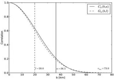
2.1 Function Co of Gaspari and Cohn compared to Gaussian Go, with l

chosen as 20 km. . . 15

3.1 Location of the observations from aircrafts (AIREP) over Italy between 9 UTC and 12 UTC on the 9th _{of October 2014. . . .} ₂₁

3.2 Location of the observations from ground stations (SYNOP) over Italy between 9 UTC and 12 UTC on the 9th _{of October 2014. . . .} ₂₂

3.3 Location of the observations from radiosondes (TEMP) over Italy be-tween 9 UTC and 12 UTC on the 9th _{of October 2014. . . .} ₂₂

3.4 COSMO-I2 domain. . . 26 3.5 Set-up of the KENDA-based data assimilation cycle. . . 26

4.1 Difference between the ensemble mean of the analysis ensemble and the ensemble mean of the background ensemble in terms of temperature at the lowest model level, with localization radius of 80 km (top) and 40 km (bottom). . . 29 4.2 Difference between the ensemble mean of the analysis ensemble and the

ensemble mean of the background ensemble in terms of temperature at the lowest model level, with localization radius of 80 km, with RTPP inflation. . . 30 4.3 Difference between the spread of the analysis ensemble and the spread

of the background ensemble in terms of mean temperature at the lowest model level, without RTPP inflation (top) and with RTPP inflation (bottom). . . 31

(12)

4.4 Difference between the ensemble mean of the analysis ensemble and the ensemble mean of the background ensemble in terms of temperature at the lowest model level, with localization radius of 80 km, with RTPS inflation. . . 32 4.5 Difference between the spread of the analysis ensemble and the spread

of the background ensemble in terms of mean temperature at the lowest model level, with RTPS inflation. . . 33 4.6 Difference between the ensemble mean of the analysis ensemble and the

ensemble mean of the background ensemble in terms of temperature at the lowest model level, with localization radius of 80 km, with SPPT scheme. . . 34 4.7 Difference between the spread of the analysis ensemble and the spread

of the background ensemble in terms of mean temperature at the lowest model level, with SPPT inflation. . . 34 4.8 Difference between the ensemble mean of the analysis ensemble and the

ensemble mean of the background ensemble in terms of temperature at the lowest model level, without AIREP data. . . 35 4.9 Difference between the ensemble mean of the analysis ensemble and the

ensemble mean of the background ensemble in terms of temperature at the lowest model level, without AIREP and SYNOP data. . . 36

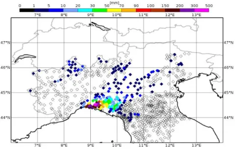
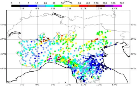
5.1 Observed precipitations accumulated over 24 hours from rain-gauge net-works on the 9th _{of October 2014. . . .} ₄₀

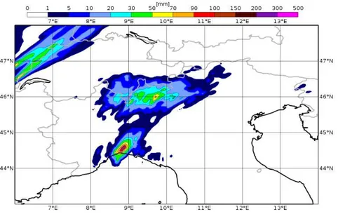
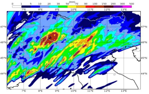
5.2 Predicted precipitations on the 9th _{of October 2014 by the deterministic}

run of COSMO model with control analysis. . . 40 5.3 Predicted precipitations on the 9th _{of October 2014 by the deterministic}

run of COSMO model with SPPT analysis. . . 41 5.4 Predicted precipitations on the 9th _{of October 2014 by the deterministic}

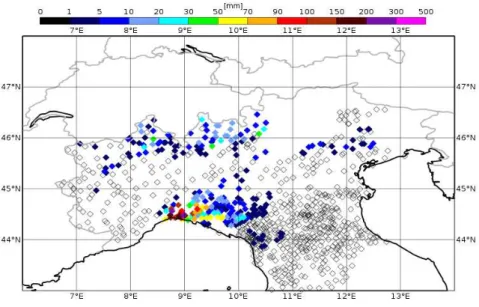
run of COSMO model with radar analysis. . . 41 5.5 Observed precipitations accumulated over 24 hours from rain-gauge

(13)

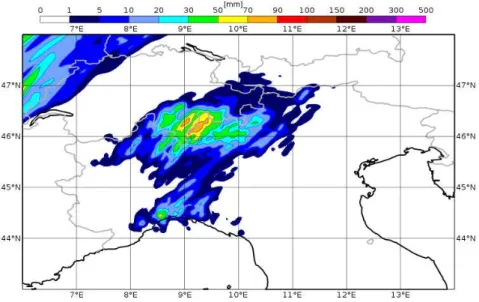
5.6 Predicted precipitations on the 10th_{of October 2014 by the deterministic}

run of COSMO model with control analysis. . . 42 5.7 Predicted precipitations on the 10th_{of October 2014 by the deterministic}

run of COSMO model with SPPT analysis. . . 43 5.8 Predicted precipitations on the 10th_{of October 2014 by the deterministic}

run of COSMO model with radar analysis. . . 43 5.9 Comparison between observed precipitations and predicted

precipita-tions on the 9th _{of October 2014. Blue line represents observed}

precipi-tations. Predicted precipitations are represented by black line (by SPPT analysis), red line (by control analysis), green line (by radar analysis). . 44 5.10 Comparison between observed precipitations and predicted

precipi-tations. Predicted precipitations are represented by black line (by SPPT analysis), red line (by control analysis), green line (by radar analysis). . 45 5.11 Observed precipitations accumulated over 24 hours from rain-gauge

net-works on the 13th _{of October 2014. . . .} ₄₆

5.12 Predicted precipitations on the 13th_{of October 2014 by the deterministic}

run of COSMO model with control analysis. . . 46 5.13 Predicted precipitations on the 13th_{of October 2014 by the deterministic}

run of COSMO model with SPPT analysis. . . 47 5.14 Predicted precipitations on the 13th_{of October 2014 by the deterministic}

run of COSMO model with radar analysis. . . 47 5.15 Comparison between observed precipitations and predicted

precipi-tations. Predicted precipitations are represented by black line (by SPPT analysis), red line (by control analysis), green line (by radar analysis). . 48 5.16 Difference between the ensemble mean of the analysis ensemble and the

ensemble mean of the background ensemble in terms of temperature at the lowest model level, on the 9th _{of October 2014 at 12 UTC, for the}

(14)

5.17 Difference between the ensemble mean of the analysis ensemble and the ensemble mean of the background ensemble in terms of temperature at the lowest model level, on the 9th _{of October 2014 at 12 UTC, for the}

SPPT analysis (top) and the radar analysis (bottom). . . 51 5.18 Temperature predicted by the control run with 20 members (top) and

40 members (bottom) before the update step (black line) and after the update step (red line) and temperature observed (green line) from a land station located in Tunisia on the 9th _{of October 2014. . . .} ₅₃

5.19 Temperature predicted by the SPPT analysis cycle (top) and by the radar analysis cycle (bottom) before the update step (black line) and after the update step (red line) and temperaute observed (green line) from a land station located in Tunisia on the 9th _{of October 2014. . . .} ₅₄

5.20 Difference between the ensemble mean of the analysis ensemble and the ensemble mean of the background ensemble in terms of temperature at level 40 of COSMO model, on the 9th _{of October 2014 at 12 UTC, for}

the control run with 20 members (top) and 40 members (bottom). . . . 56 5.21 Difference between the ensemble mean of the analysis ensemble and the

ensemble mean of the background ensemble in terms of temperature at level 40 of COSMO model, on the 9th _{of October 2014 at 12 UTC, for}

the SPPT analysis (top) and radar analysis (bottom). . . 57 5.22 Difference between the ensemble mean of the analysis ensemble and the

ensemble mean of the background ensemble in terms of temperature at the lowest level of the model, on the 13th _{of October 2014 at 12 UTC,}

for the control run with 20 members (top) and 40 members (bottom). . 59 5.23 Difference between the ensemble mean of the analysis ensemble and the

ensemble mean of the background ensemble in terms of temperature at the lowest level of the model, on the 13th _{of October 2014 at 12 UTC,}

(15)

5.24 Temperature predicted by the control run with 20 members (top) and radar analysis (bottom) before the update step (black line) and after the update step (red line) and temperature observed (green line) from a land station located in Switzerland on the 13th _{of October 2014. . . . .} ₆₂

5.25 Temperature predicted by the control run with 20 members (top) and radar analysis (bottom) before the update step (black line) and after the update step (red line) and temperature observed (green line) from a land station located in Bologna on the 13th _{of October 2014. . . .} ₆₃

5.26 Temperature predicted by the control run with 20 members (top) and 40 members (bottom) before the update step (black line) and after the update step (red line) and temperature observed (green line) from a land station located in Switzerland from the 7th _{to the 14}th _{of October 2014.} ₆₆

5.27 Temperature predicted by the SPPT analysis (top) and radar analysis (bottom) before the update step (black line) and after the update step (red line) and temperature observed (green line) from a land station located in Switzerland from the 7th _{to the 14}th _{of October 2014. . . . .} ₆₇

5.28 Representation of rmse (black line), bias (red line) and spread (green line) of the temperature after the update step, for the control run with 20 members (top) and 40 members (bottom). . . 69 5.29 Representation of rmse (black line), bias (red line) and spread (green

line) of the temperature after the update step, for the SPPT analysis (top) and radar analysis (bottom). . . 70 5.30 Observational error (black), spread (red), mean error of observation

-first guess (green), mean squared error of observation - -first guess (blue) for observations by radiosondes. Observations are in terms of temperature. 73 5.31 Observational error (black), spread (red), mean error of observation

-analysis (green), mean squared error of observation - -analysis (blue) for observations by radiosondes. Observations are in terms of temperature. 73 5.32 Observational error (black), spread (red), mean error of observation

-first guess (green), mean squared error of observation - -first guess (blue) for observations by radiosondes. Observations are in terms of wind. . . 74

(16)

5.33 Observational error (black), spread (red), mean error of observation -analysis (green), mean squared error of observation - -analysis (blue) for observations by radiosondes. Observations are in terms of wind. . . 74 5.34 Observational error (black), spread (red), mean error of observation

-first guess (green), mean squared error of observation - -first guess (blue) for observations by airplanes. Observations are in terms of temperature. 75 5.35 Observational error (black), spread (red), mean error of observation

-analysis (green), mean squared error of observation - -analysis (blue) for observations by airplanes. Observations are in terms of temperature. . . 75 5.36 Observational error (black), spread (red), mean error of observation

-first guess (green), mean squared error of observation - -first guess (blue) for observations by airplanes. Observations are in terms of wind. . . 76 5.37 Observational error (black), spread (red), mean error of observation

-analysis (green), mean squared error of observation - -analysis (blue) for observations by airplanes. Observations are in terms of wind. . . 76 5.38 Observational error (red), mean error (black), mean squared error (blue)

for observations by land stations. Observations are in terms of wind. . . 77 5.39 Observational error (red), mean error (black), mean squared error (blue)

for observations by land stations. Observations are in terms of surface pressure. . . 77 5.40 Spread before update step (red line), mean error of observation - first

guess (green line), mean error of observation - analysis (dashed green line), mean squared error of observation - first guess (blue line), mean squared error of observation - analysis (dashed blue line), for observa-tions by radar. Observaobserva-tions are in terms of reflectivity. . . 78

(17)

Introduction

Forecasting a physical system generally requires both a model for the time evolution of the system and an estimate of the current state of the system. In some applications, such as weather forecasting, direct measuraments of the global system state is not fea-sible, but it must be inferred from available data.

While a reasonable state estimate based on current data may be possible, in general one can obtain a better estimate by using both current and past data (Hunt et al., 2007).

Data assimilation is an analysis technique in which the observations are accumulated into the model state and propagate to all variables of the model. Many assimila-tion techniques, such as Cressman analysis, Optimal interpolaassimila-tion analysis, Three-dimensional (3D-Var) and four-Three-dimensional (4D-Var) variational assimilation, Local Ensemble Transform Kalman Filter (LETKF), have been developed for meteorology and oceanography. They differ in terms of numerical cost, their optimality and their suitability for real-time data assimilation (Bouttier and Courtier, 1999).

The aim of this work is to assess the impact of the assimilation of conventional data and radar data in a LETKF scheme, analizing the dependency on the parameters of the scheme (localization radius, inflation method, data density).

An experimental kilometer-scale ensemble data assimilation (KENDA) system for the COnsortium for Small-scale MOdeling (COSMO) forecast model has been developed at Deutscher Wetterdienst (DWD) (Harnisch and Keil, 2015; Schraff et al., 2016). The general purpose is to provide initial conditions to the high-resolution applications of the COSMO model both in deterministic and in ensemble system. The LETKF data assimilation scheme produces an analysis ensemble that gives a theoretical estimate of the analysis uncertainty and which can be used to initialize a forecast ensemble

(18)

(Har-nisch and Keil, 2015).

A deterministic analysis is also produced, which can be used as initial condition to the deterministic model run.

In the present work, some experiments have been done over one week in October 2014, including 9th _{and 13}th _{October, when two major flood events took place respectively}

in Genova and Parma. The quality of the different analyses as well as their impact in initializing the deterministic forecast have been evaluated both on case studies and statistically over the entire period.

(19)

Chapter 1 Data assimilation

1.1 General problem of Data Assimilation

Data assimilation is an iterative approach to the problem of estimating the state of a dynamical system using both current and past observations of the system together with a model for the system time evolution.

This model can be used to “forecast” the current state, using a prior state estimate (which incorporates information from past data) as the initial condition. After that, current data are used to correct the prior forecast to a current state estimate. This is the Bayesian approach, that is most effective when the uncertainty (both in the obser-vations and in the state estimate) is quantified (Hunt et al., 2007). Data assimilation is an analysis technique in which the observed information is accumulated in time into the model state, and it propagates to all variables of the model. This technique is widely used to study and forecast geophysical systems.

An analysis is the production of an accurate image of the true state of the atmosphere, represented in a model as a collection of numbers (Bouttier and Courtier, 1999). The basic information used to produce the analysis is a collection of observed values provided by observations of the true state. In most cases the analysis problem is under-determined because data is sparse and only indirectly related to the model variables. In order to make it a well-posed problem, it is necessary to rely on some background information in the form of a priori estimate of the model state. The background in-formation can be a climatology state; it can also be generated from the output of a

(20)

previous analysis, using some assumptions of consistency in time of the model state. There are two basic approaches to data assimilation: sequential assimilation and non-sequential (retrospective) assimilation. The first one, only considers observation made in the past until the time of analysis, that is the case of real-time assimilation system, while the second one considers observation from the future, for example in a reanal-ysis exercise. Another distinction can be made between intermittent and continuous assimilation. In an intermittent assimilation, observations can be processed in a small batches, which is technically convenient. In a continuous assimilation, observation batches over longer periods are considered, and the correction to the analysis state is smooth in time, which is physically more realistic (Bouttier and Courtier, 1999; Daley, 1991; Ghil, 1989).

Data assimilation iteratively alternates between a forecast step and a state estimation step (also called “analysis”). The analysis step is a statistical procedure involving a prior estimate (background) of the current state based on past data, and current data (observations) which are used to improve the state estimate. This procedure requires quantification of the uncertainty both in the background state and in the observations. There are two main factors creating background uncertainty: one is the uncertainty in the initial conditions from the previous analysis, the other is the “model error”, the unknown discrepancy between the model dynamics and actual system dynamics (Hunt

et al., 2007). The emphasis here is on methodology used in data assimilation.

Ideally, it can be kept track of a probability distribution of system states, propagat-ing the distribution uspropagat-ing the Fokker-Planck-Kolmogorov equation durpropagat-ing the forecast step. This approach provides a theoretical basis for the methods used in practice (Jazwinski, 1970), but it would be computationally expensive and is not feasible for a high-dimensional system. Instead, it can be used the Monte Carlo approach, using a large ensemble of system states to approximate the distribution (Doucet et al., 2001), or an approach like the Kalman Filter (Kalman, 1960; Kalman et al., 1961) that as-sumes Gaussian distributions and tracks their mean and covariance.

Ensemble Kalman Filter (Evensen, 1994; Evensen, 2003; Evensen, 2006) has elements of both approaches: it uses the Gaussian approximation and follows the time evolution of the mean and the covariance by propagating an ensemble of states.

(21)

The ensemble should be large enough to span the space of possible system states at a given time, because the analysis determines essentially which linear combination of the ensemble members forms the best estimate of the current state, given the current observations.

1.2 Bayesian update

The aim of the Bayesian data assimilation is to estimate the probability density function (pdf) for the current atmospheric state given all current and past observations. When considering Bayesian assimilation, assuming that a pdf of the state of the atmosphere is available, there are two steps to the assimilation: the first step is to assimilate recent observations, thereby sharpening the pdf, the second step is to propagate the pdf forward in time until new observations are available. If the pdf is initially sharp (i.e. the distribution is relatively narrow), chaotic dynamics and model uncertainty will usually broaden the probability distribution (Anderson and Anderson, 1999; Hamill, 2006).

Assuming that an estimate of the pdf has been propagated forward to a time when observations are available, the state can be estimate more specifically by incorporating information from the new observations.

It is now possible to use the following notational convention: xt

t−1 denotes the

n-dimensional true model state at time t-1, ψt = [yt, ψt−1] is a collection of observations,

where ytare the observations at the most recent time and ψt−1 are the observations at

all previous times.

The update problem is to accurately estimate P (xt

t|ψt), which is the probability density

estimate of the current atmospheric state, given the current and past observations. According to Bayes’ rule: P (xt

(22)

Assuming that observation errors are independent from one time to the next:

P(ψt|xtt) = P (yt|xtt)P (ψt−1|xtt),

therefore:

P(xt

t|ψt) α P (yt|xtt)P (ψt−1|xtt)P (xtt),

which applying the Bayes’ rule becomes:

P(xt

t|ψt) α P (yt|xttP(xtt|ψt−1).

The term on the left-hand side P (xt

t|ψt) is the pdf for the current model state given

all the observations (“posterior”). The first term on the right-hand side P (yt|xtt) is

the probability distribution for the current observations. The second term on the right-hand side P (xt

t|ψt−1) is the pdf of the model state at time t given all the past

observations up to time t-1 (“prior” or “background”). Without some simplification, full Bayesian assimilation is computationally impossible for model state of large dimension. Assuming normality of error statistics and linearity of error growth, the state and its error covariance may be predicted using Kalman Filter techniques.

1.3 Ensemble Kalman Filter

Ensemble-based data assimilation techniques are used as possible alternatives to op-erational analysis techniques such as three-dimensional (3D-Var) or four-dimensional variational assimilation (4D-Var).

3D-Var (Lorenc, 1981; Parrish and Derber, 1992) is a method in which data assimila-tion is performed every 6 hours, and in the cost funcassimila-tion, the background covariance Pb is replaced by a constant matrix B representing typical uncertainty in a 6-hour fore-cast. The 4D-Var method (Le Dimet and Talagrand, 1986; Talagrand and Courtier, 1987) uses a cost function that includes a constant covariance background as in 3D-Var, together with a sum accounting for the observations collected over a 12-hour time window. The cost function is minimized; this is computationally expensive because computing the gradient of the cost function requires integrating both the nonlinear

(23)

model and its linearization over 12-hour, and this is repeated until a satisfactory ap-proximation to the minimum is found.

The Ensemble Kalman Filter is an approximation to the Kalman Filter in that background-error covariances are estimated from a finite ensemble of forecasts. Background background-error covariances are estimated using the forecast ensemble and are used to produce an en-semble of analysis; these covariances are flow dependent and often have complicated structure.

Even though Ensemble-based techniques are computationally expensive, they are rel-atively easy to code (Hamill, 2006).

The key idea of Ensemble Kalman Filter (Evensen, 1994; Evensen, 2006) is to choose at time tn−1 an ensemble of initial conditions whose spread around xa (at time tn−1)

characterizes the analysis covariance Pa_{, propagate each ensemble member using the}

nonlinear model, and compute Pb _{based on the resulting ensemble at time t}

n. The

uncertainty in the state estimate is propagated from one analysis to the next, like the extended Kalman Filter. Instead, 3D-Var method does not propagate the uncertainty, while 4D-Var method propagates it only with the time window over which the cost function is minimized.

The most important difference between Ensemble Kalman Filtering and the other meth-ods is that the former quantifies uncertainty only in the space spanned by the ensemble. A possible limitation is that computational resources restrict the number of ensemble members (k) to be much smaller than the number of variables of the model (m), but, if this limitation can be overcome (see 2.3.1), the analysis can be performed in a much lower-dimensional space. Thus, Ensemble Kalman Filtering has the potential to be more computationally efficient than the other methods.

1.3.1 Comparison between Ensemble-based method and

4D-Var variational assimilation

Some intelligent guesses can be made regarding advantages and disadvantages of Ensemble-based method and 4D-Var method (Lorenc, 2003).

Ensemble-based methods are much easier to code and maintain than the 4D-Var varia-tional assimilation. Ensemble-based methods produce an ensemble of possible analysis

(24)

states, providing information about both the mean analysis and its uncertainty, there-fore, an advantage of using this method is that the ensemble of analysis state can be used directly to initialize ensemble forecasts without any additional computations. Another advantage is that if the analysis uncertainty is very spatial inhomogeneous and time dependent, in Ensemble-based methods this information will be fed through the ensemble from one assimilation cycle to the next. Instead, in 4D-Var, the assim-ilation typically starts at each update cycle with the same stationary model of error statistics. Consequently, the influence of observations can be more properly weighted in Ensemble-based methods than in 4D-Var.

Ensemble-based methods also provide a direct way to incorporate the effects of model imperfections directly into the data assimilation. In 4D-Var, differently, the forecast model dynamics are a strong constraint (Courtier et al., 1994). If the forecast model used in 4D-Var does not adequately represent the true dynamics of the atmosphere, model error can be large, and it may fit a model trajectory very different from the trajectory of the real atmosphere.

On the other hand, a disadvantage of Ensemble-based methods is that are at least as computationally expensive as 4D-Var, and perhaps more expensive when there is an overwhelmingly large number of observations (Hamill and Snyder, 2000; Etherton and Bishop, 2004). Furthermore, ensemble approaches may be difficult to apply in lim-ited area models because of difficulty of specifying an appropriate ensemble of lateral boundary conditions.

(25)

Chapter 2 Ensemble Kalman Filter

2.1 Kalman Filter

The problem of which trajectory of a dynamical system best fits a time series of data, is solved exactly for linear problems by using the Kalman Filter and approximately for nonlinear problems by using Ensemble Kalman Filters.

It will be described how to perform a forecast step from time tn−1 to tn, followed by an

analysis step at time tn, in such a way that if we start with the most likely system state,

given the observations up to time tn−1, we end up with the most likely state given the

observations up to time tn. The forecast step propagates the solution from time tn−1

to tn, and the analysis step combines the information provided by the observations at

time tn with the propagated information from the prior observations. The first step

is to assume that the analysis at time tn−1 has produced a state estimate xan−1 and

an associated covariance matrix Pa

n−1. They represent respectively the mean and the

covariance of a Gaussian probability distribution that represents the relative likelihood of the possible system states given the observations from time tn−1to tn. Algebraically

(Hunt et al., 2007), it can be written:

Pn−1 j=1[yjo− HjMtn−1,tjx] T_R−1 j [yjo− HjMtn−1,tjx] = [x − ¯x a n−1]T(Pn−1a )−1[x − ¯xan−1] + c,

where x is a m-dimensional vector representing the state of the system at a given time, yo

j is a vector of observed values, M is the model forecast operator, R is the covariance

matrix, H is the observation operator that describes the relationship between yo j and

(26)

x(tj): yoj = Hj(x(tj)), and c is a constant.

The following step is to propagate the analysis state estimate ¯xa

n−1 and its covariance

P_n−1a , by using the model forecast operator M to produce a background estimate ¯xb_n and its covariance Pb

n: ¯ xb_n= Mtn−1,tnx¯ a n−1 and Pnb = Mtn−1,tnP a n−1MtTn−1,tn.

The next step is the minimization of a cost function, so that it is possible to estimate the state at time tn:

Jtn(x) = (x − ¯x

b

n)T(Pnb)−1(x − ¯xbn) + (yno − Hnx)TR−1n (yno − Hnx) + c.

The analysis state estimate ¯xa _{and its covariance P}a _{at time t} n are: ¯ xa n= ¯xbn+ PnaHnTRn−1(yno− Hnx¯bn), P_na= (I + Pb nHnTR−1n Hn)−1Pnb, with Pa

nHnTR−1n called “Kalman gain”.

Many approaches to data assimilation for nonlinear problems are based on Kalman Filter. A nonlinear model forces a change in the equations calculating ¯xb

n and Pnb,

while nonlinear observation operators Hn force a change in the calculation of ¯xan and

Pa n.

2.2 Ensemble Kalman Filter

Ensemble Kalman Filter is the most well-known stochastic ensemble data assimilation algorithm. This algorithm updates each member to a different set of observations per-turbed with random noise. Because randomness is introduced every assimilation cycle, the update is considered stochastic.

We start with an ensemblen

xa(i)_n−1 : i = 1, 2, ..., koof m-dimensional model state vectors at time tn−1. The ensemble is chosen so that its average represents the analysis state

(27)

background ensemble n xb(i)_n : i = 1, 2, ..., ko at time tn: xb(i) n = Mtn−1,tn(x a(i) n−1).

For the background state estimate and its covariance, the sample mean ¯xb _and

covari-ance Pb _{of the background ensemble are used:}

¯

xb = k−1Pk

i=1xb(i) and

Pb _{= (k − 1)}−1Pk

i=1(xb(i)− ¯xb)(xb(i)− ¯xb)T = (k − 1)−1Xb(Xb)T.

Xb is the m x k matrix whose i-th column is xb(i)_{− ¯x}b. Unlike the Kalman Filter or 3D-Var, the background error covariance estimate is generated from an ensemble of non-linear forecasts. These background error covariances can vary in time and space. For the analysis state estimate and its covariance, the sample mean ¯xa _{and covariance}

Pa are used:

¯

xa_{= k}−1Pk

i=1xa(i),

Pa_{= (k − 1)}−1Pk

i=1(xa(i)− ¯xa)(xa(i)− ¯xa)T = (k − 1)−1Xa(Xa)T,

where Xa _{is the m x k matrix whose i-th column is x}a(i)_{− ¯x}a_.

2.3 Local Ensemble Transform Kalman Filter

In the LETKF (Hunt et al., 2007), an ensemble of forecasts is used to represent a situation-dependent background error covariance. This is implicitly deployed then in three steps taking into account the observations and their errors. Firstly, the analysis mean state (best linear unbiased estimate) is equal to the ensemble mean forecast plus a weighted sum of the forecast perturbations (i.e. the deviations of the individual ensem-ble forecasts from the ensemensem-ble mean forecast) where the weights depend on the devia-tions of the ensemble members to the observadevia-tions. Secondly, the analysis covariance is calculated. Thirdly, the analysis perturbations are determined as a linear combination of the forecast perturbations such that they reflect the analysis covariance. Asynoptic, high-frequency, and indirect observations can also be accounted for (COSMO web site,

(28)

http://www.cosmo-model.org/content/tasks/pastProjects/kenda/default.htm). Local-isation, e.g. by using only observations in the vicinity of a certain grid point, requires the ensemble to represent uncertainty in only a rather lower-dimensional local unstable sub-space. This reduces the sampling errors (i.e. the errors in sampling the forecast errors) and rank deficiency (which expresses that due to the limited ensemble size, the ensemble is not able to explore the complete space of uncertainty in general). Note that the method provides a framework how to make smooth transitions between different linear combinations of the ensemble members in different regions (e.g. by gradually increasing the specified observation errors with increasing distance from the observa-tion). This should allow to keep both the ensemble size and the imbalances caused by localisation reasonably small (cosmo-model.org site web).

The LETKF method is now described, which is an efficient means of performing the analysis that transforms a background ensemble xb(i) _{into an appropriate analysis}

en-semble xa(i)_{. It has been assumed that the number of ensemble members k is smaller}

than the number of model variables m. We want the analysis mean ¯xa _{to minimize}

the Kalman Filter cost function used in a linear scenario, modified to allow for a non linear observation operator H:

J_{(x) = (x − ¯x}b₎T_(Pb₎−1_{(x − ¯x}b_{) + [y}o_{− H(x)]}T_R−1_[yo_{− H(x)].}

H(x) is the observation operator: it acts as a collection of interpolation operators from the model discretization to the observation points. This operator is important because generally, there are fewer observations than variables in the model and they are not reg-ularly disposed, so that the only way to compare observations with the state vector is through the use of H(x). Another important step is the passage from a m-dimensional system to a k-dimensional system, with the aim to reduce the number of variables in the system. In this new space, if w is a Gaussian random vector with mean 0 and covariance (k − 1)−1_{I, then x = ¯x}b _{+ X}b_w _{is Gaussian with mean ¯x}b _{and covariance}

(29)

In the transformed space, the cost function becomes:

J_{(w) = (k − 1)w}T_w_{+ [y}o_{− H(¯x}b_{+ X}b_w)]T_R−1_[yo_{− H(¯x}b_{+ X}b_w)].

If ¯wa minimizes J(w), ¯xa = ¯xb+ Xb_w_¯a _{minimizes the cost function J.}

Beacuse we only need to evaluate the observation operator H in the ensemble space, the simplest way to linearize H is to apply it to each of the ensemble members xb(i)

and interpolate. It has defined an ensemble yb(i)_{of background observation vectors by}

yb(i)= H(xb(i)_).

Another important step is the linear approximation:

H(¯xb+ Xb_w_{) ≈ ¯y}b_{+ Y}b_w.

By substituting this term into the cost function J(w) is possible to obtain:

˜

J_{(w) = (k − 1)w}Tw+ [yo_{− ¯y}b_{+ Y}b_w]T_R−1_[yo_{− ¯y}b_{− Y}b_w].

In transformed space, the analysis equations are:

¯

wa= ˜Pa(Yb₎T_R−1_(yo_{− ¯y}b_{) and}

˜

Pa_{= [(k − 1)I + (Y}b₎T_R−1_Yb_]−1_.

In model space, the analysis mean and covariance are:

¯

xa_{= ¯}_xb_{+ X}b_w_¯a_,

Pa= Xb_P_˜a_(Xb₎T_.

To initialize the ensemble forecast that will produce the background for the next anal-ysis, it must be chosen an analysis ensemble whose sample mean and covariance are respectively ¯xa _{and P}a_{. It can be formed the analysis ensemble by adding ¯x}a _{to each}

of the columns of Xa_.

A good choice of analysis ensemble is described by Xa _{= X}b_Wa_{, where}

Wa_{= [(k − 1) ˜}Pa]1/2_.

The use of symmetric root to determine Wa _{from ˜}_Pa _{is important for two reasons:}

(30)

analy-sis ensemble has the correct sample mean (Wang et al., 2004). The second reason is that it ensures that Wa _{depends continuously on ˜}_Pa_{. This is very important, so that}

neighboring grid points with slightly different matrices ˜Pa do not yield very different analysis ensembles. It is possible to form the analysis ensemble by adding ¯wa _{to each}

of the columns of Wa_. n

wa(i)o are the columns of the resulting matrix. These weights vector specify what linear combinations of the background ensemble perturbations to add to the background mean to obtain the analysis ensemble in model space:

xa(i)_{= ¯}_xb_{+ X}b_wa(i)_.

2.3.1 Localization

Another important issue in Ensemble Kalman Filter is the spatial localization. If the ensemble has k members, the background covariance matrix given by Pb _describes

un-certainty only in the k-dimensional subspace spanned by the ensemble, and a global analysis will allow adjustments to the system state only in this subspace. If the system is high-dimensionally unstable (if it has more than k positive Lyapunov exponents), the forecast errors will grow in direction not accounted for by the ensemble, and these errors will not be corrected by the analysis (Hunt et al., 2007).

Another problem could be that the limited sample size provided by an ensemble will produce spurious correlations between distant locations in the background covariance matrix Pb _{(Houtekamer and Mitchell, 1998; Hamill et al., 2001). These spurious}

cor-relations will cause observations from one location to affect, in a random manner, the analysis in localizations a large distance away.

About localization, it is important to point out that is generally done implicitly, by multiplying the entries in Pb _{by a distance-dependent function that decays to zero}

be-yond a certain distance, so that observations do not affect the model state bebe-yond that distance (Houtekamer and Mitchell, 2001; Hamill et al., 2001; Whitaker and Hamill, 2002).

In particular the implementation in KENDA is as follows.

For every point of the analysis grid, a local ensemble of model equivalents n

yb(i)o with corresponding local observations yo

(31)

in the inverse observation error covariance matrix R−1 _{are multiplied with a}

distance-dependent correlation function Co. Therefore, the single observations yiowill contribute

to the local analysis, at every point, with an observation weight ≤ 1.

The function Co is a polynomial approximation to a Gaussian function Go = exp(−b

2

2l2),

where b is the spatial distance between the single analysis grid point and the location of one single observation, and l is the length scale where Go = exp(−1₂) ≈ 0.61.

The localization radius is rloc = 2l

q

10

3 , where the function Co goes to zero (Gaspari

and Cohn, 1999; Hamill et al., 2001). The input parameter l is typically chosen ample enough to overlap with neighboring analysis grid points in order to obtain a spatially smooth field of local analysis weightsnwa(i)o_{. Observations that are further away than}

rloc are neglected, while the observation weights are very close to a Gaussian curve

(Documentation of the DWD Data Assimilation System, available on request).

Figure 2.1: Function Co of Gaspari and Cohn compared to Gaussian Go, with l chosen

as 20 km.

2.3.2 Covariance inflation

An inflation procedure needs to be applied to account for unrepresented systematic errors in the Local Ensemble Transform Kalman Filter, such as model or sampling errors. These systematic errors lead to an underestimation of the background ensemble

(32)

variance which subsequently decreases the weight given to the observations. If this discrepancy becomes too large it can happen that no weight is given to the observations and that they are essentially ignored.

A number of procedures are developed to counteract this problem, and they can be separated into additive and multiplicative methods. The additive methods add some multiples of the identity matrix to the background or analysis covariances (Ott et al., 2004), while the multiplicative methods multiply background or analysis covariances by a factor larger than 1 (Anderson and Anderson, 1999; Hamill et al., 2001). In case each analysis member has a corresponding background member, relaxation methods can also be applied where the inflations relaxes the analysis ensemble back towards the background ensemble.

2.3.2.1 Multiplicative covariance inflation

The multiplicative covariance inflation can be applied on either the background or the analysis covariance in each data assimilation cycle. It can be performed on the analysis by multiplying the analysis perturbations by an appropriate inflation factor ρ during the data assimilation step. Even the background ensemble can be inflated by multiplying the background perturbations by some factor ρ before the data assimilation.

2.3.2.2 Relaxation of the analysis ensemble

This alternative approach inflates the ensemble by relaxing the analysis ensemble to-wards the background ensemble. There are two types of relaxation: relaxation to prior perturbations (RTPP) and relaxation to prior spread (RTPS).

By using the first type, the analysis ensemble perturbations are relaxed back to the background values (Zhang et al., 2004). These perturbations Xa _{are relaxed}

indepen-dently at each grid point:

Xa_{← (1 − α)X}a_{+ αX}b_.

The analysis ensemble perturbation matrix Xa _{is defined as the column matrix of the}

differences of the k-th analysis ensemble member from the analysis ensemble mean. The background ensemble perturbation matrix is defined in the same way. By using

(33)

the second type, instead of relaxing the perturbations, the analysis ensemble spread is relaxed back to the background ensemble spread (Whitaker and Hamill, 2012).

The analysis ensemble standard deviation is relaxed back to the background values at each grid point:

σa _{← (1 − α)σ}a+ ασb_,

where σa₌q_{(K − 1)}−1PK

k=1(Xa)2 and σb =

q

(K − 1)−1PK

k=1(Xb)2 denote the

anal-ysis and background ensemble standard deviation respectively, and K is the ensemble size. By using the last two equations, it can be written:

Xa_{← X}a(ασb_−σa

σa + 1).

The notation of α is used to represent the inflation factor for RTPP and RTPS method because in both cases it represents a relaxation of the analysis ensemble to the back-ground ensemble. The factor α is a tunable parameter, and it has been found an optimal value of 0.755 for the RTPP method and 0.95 for the RTPS method (Whitaker and Hamill, 2012).

2.3.2.3 Stochastically Perturbed Parametrization Tendencies

The Stochastically Perturbed Parametrization Tendencies (SPPT) scheme perturbs the total parametrized tendency of physical processes (as opposed to the dynamics). The original SPPT scheme perturbs the net parametrized tendency of physical pro-cesses of the model (turbulence, radiation, shallow convection, microphysics...) by using multiplicative noise during run time (Buizza et al., 1999). The tendencies of the wind components u, v, temperature T and humidity q are perturbed. For an unper-turbed tendency Xc, the perturbed tendency Xp is computed as:

Xp = (1 + rX)Xc

where rX is a random number drawn from a uniform distribution in the range [−0.5, 0.5].

The perturbations are multivariate, i.e. different random numbers are used for the four variables (u, v, T, q). The same random numbers are used in the whole column over boxes of pre-defined size, 5◦ _{by 5}◦ _{in latitude and longitude in the implementation}

(34)

adopted for the present work.

The revised SPPT scheme uses perturbations collinear to the unperturbed tendencies Xc. The perturbed tendency is computed as:

Xp = (1 + rµ)Xc

where r si the same randum number. The factor µ ∈ [0, 1] is used for reducing the perturbation amplitude close to the surface and in the stratosphere. The replacement of the multivariate perturbations by a univariate Gaussian distribution is an attempt to introduce perturbations that are more consistent whit the model physics, in particular, this change is designed to address the overprediction of heavy precipitation events.

(35)

Chapter 3 The LETKF Data Assimilation of the

COSMO COnsortium

3.1 The KENDA System

The Kilometer-scale ENsemble Data Assimilation system (KENDA), based on a Local Ensemble Transform Kalman Filter, has been developed for the kilometer-scale configu-ration of the COnsortium for Small-scale MOdeling (COSMO, www.cosmo-model.org) limited area model.

The main purpose of this data assimilation scheme is to provide the initial conditions both for deterministic and ensemble forecasting systems which are run at a convection permitting resolution. A description of the KENDA Project is available at www.cosmo-model.org/content/tasks/pastProjects/kenda/default.htm.

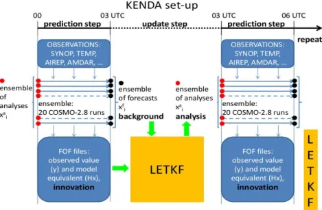
LETKF alternates between a prediction step and an update step (analysis). The pre-diction step consists of an ensemble of COSMO runs which produces the background ensemble and is followed by an update step, when the KENDA code is run to produce the 20 perturbed analyses.

During the COSMO model integration, observations are read and model equivalent is computed for each ensemble member using the observation operator which is different for each of observation type.

In KENDA the analysis for a deterministic data assimilation and forecast cycle is also implemented, and it is determined by applying the Kalman gain matrix for the

(36)

ensem-ble mean to the innovations of the unperturbed deterministic (or control) run:

xa_{= x}b_+LXb_P˜a_(Yb₎T_R−1_(yo_−H(xb_{)). The rationale of using the gain of the ensemble}

mean is that both, the ensemble mean and the deterministic analysis, aim to provide an unperturbed best estimate of the true state. It allows the deterministic analysis to take full advantage of the flow-dependent ensemble background covariances. The deterministic analysis will not be optimal if its background deviates significantly from the background ensemble mean (Schraff et al., 2016).

3.2 Observations

3.2.1 Conventional data: AIREP, TEMP, SYNOP

The conventional observation types which can be assimilated in KENDA are in-situ observations and surface observations. In-situ observations directly measure the at-mospheric quantities temperature, pressure, wind components u and v and specific humidity within the atmosphere.

In-situ observations are provided by airplanes (AIREP report) and radiosondes (TEMP report).

The observation operator for in-situ observations consists of vertical and horizontal interpolation. The vertical interpolation is an interpolation to the pressure level of the observation, and is performed in terms of temperature, generalised humidity and wind components u and v. Horizontal interpolation is an interpolation to the location of the observation, and it is a bi-linear interpolation used for all quantities (Documentation of the DWD Data Assimilation System, available on request).

Surface observations are observations from weather stations close to the surface, e.g. at 2 or 10 meter height (SYNOP report). SYNOP data are the weather measurements obtained from land stations and ships. Meteorological quantities provided by SYNOP data are temperature, moisture, cloud state, dew point, wind speed and direction, visibility, pressure, weather state, precipitation and snow state and dynamics. Near surface temperature is not assimilated because it strongly depends on the surface char-acteristics and is not representative for the temperature in the atmosphere. Unlike

(37)

in-situ observations, the observation operator consists of horizontal interpolation only. Observations used in the assimilation are denoted as ACTIVE or ACCEPTED. The ACCEPTED flag indicates that the observation obtained a weight larger than 0.5 in the Variational Quality Control (VQC). Instead, the ACTIVE flag indicates that the observation obtained a weight smaller than 0.5 in the VQC.

Observations not used in the assimilation are denoted as REJECTED if they are dis-missed due to insufficient quality (did not pass all of the quality control checks). They are denoted as PASSIVE if they are not assimilated but processed by the assimilation system just for monitoring purposes. The PASSIVE-REJECTED flag indicates that passivly monitored observations did not pass the quality control checks. Observations denoted as DISMISSED are rejected without being written to any of the monitoring file. The status MERGED refers to reports that were merged into others.

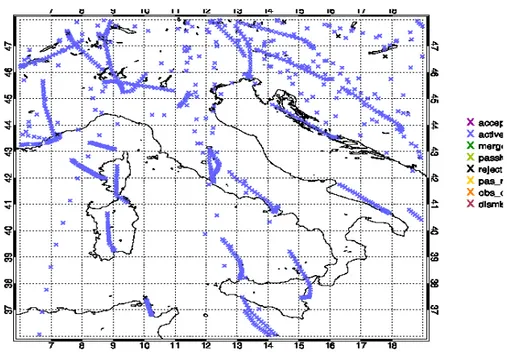
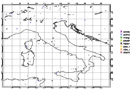
In figures 3.1, 3.2 and 3.3 are shown respectively the location of the observations from aircrafts (AIREP), ground stations (SYNOP) and radiosondes (TEMP) over Italy be-tween 9 UTC and 12 UTC on the 9th _{of October 2014. They are flagged as ACTIVE}

(blue crosses) and REJECTED (black crosses).

Figure 3.1: Location of the observations from aircrafts (AIREP) over Italy between 9 UTC and 12 UTC on the 9th _{of October 2014.}

(38)

Figure 3.2: Location of the observations from ground stations (SYNOP) over Italy between 9 UTC and 12 UTC on the 9th _{of October 2014.}

Figure 3.3: Location of the observations from radiosondes (TEMP) over Italy between 9 UTC and 12 UTC on the 9th _{of October 2014.}

(39)

3.2.2 Non conventional data: radar reflectivity

In KENDA it is possible to assimilate also 3d volumes of data reflectivity thanks to the Radar Forward Operator (RFO, Zeng et al., 2012).

The Radar Forward Operator computes the model equivalent of the radar reflectivity using the prognostic variables of the COSMO model given on the model grid. In par-ticular, for further calculations it uses the three-dimensional wind components (u, v, w), the temperature T and informations on hydrometers: it is possible to distinguish between cloud droplets, cloud ice, raindrops, snow and graupel by using their mass densities. The following step is the calculation of the temperature dependent refractive index m of the particles, the degree of melting and the shape of hydrometeors. It is now possible to calculate radar reflectivity factor Ze on model grid:

Ze= ηλ

4

π5

|Kw|2,

with η radar reflectivity, λ wavelength of the radar, Kw reference value of the dieletric

constant of water. The radar reflectivity can be calculated by using either Rayleigh or Mie theory. The Rayleigh theory is simpler and more efficient than the Mie theory. However, using Mie theory, it is also possible to calculate the extinction coefficient. The Radar Forward Operator works on parallel supercomputer architectures, therefore parallelisation strategy is used: the radar volume is divided in horizontal interpolated "azimuthal slices" evenly distributed.

In the next step, the Radar Operator calculates the propagation of radar beam con-sidering beam bending due to atmospheric refraction. Another step is the vertical interpolation of values of reflectivity, extinction and model wind from model grid onto the radar beam. Then, the attenuation of the radar reflectivity due to atmospheric hydrometeors can be calculated. Every observable is now avalaible on the radar beam lying on a single line along the beam axis. A beam weighting function is used for the increasing pulse volume with distance (Zeng et al., 2012).

(40)

3.3 The COSMO model

The COSMO-Model is a nonhydrostatic limited-area atmospheric prediction model (www.cosmo-model.org). It has been designed for both operational numerical weather prediction (NWP) and various scientific applications on the meso-β and meso-γ scale. The COSMO-Model is based on the primitive thermo-hydrodynamical equations de-scribing compressible flow in a moist atmosphere. The model equations are formulated in rotated geographical coordinates and a generalized terrain following height coor-dinate. A variety of physical processes are taken into account by parameterization schemes.

A variety of subgrid-scale physical processes are taken into account by parameterization schemes: Grid-Scale Clouds and Precipitation, Subgrid-Scale Clouds, Moist Convec-tion, RadiaConvec-tion, Subgrid-Scale Orography, Subgrid-Scale Turbulence, Surface Layer, Soil Processes, Sea Ice Scheme, Lake Model.

The basic version of the COSMO-Model (formerly known as Lokal Modell, LM) has been developed at the Deutscher Wetterdienst (DWD). The COSMO-Model and the triangular mesh global gridpoint model GME form (together with the corresponding data assimilation schemes) the NWP-system at DWD, which is run operationally since end of 1999. The subsequent developments related to the model have been organized within COSMO, the Consortium for Small-Scale Modelling. COSMO aims at the improvement, maintenance and operational application of the non-hydrostatic limited-area modelling system, which is now consequently called the COSMO-Model.

By employing 1 to 3 km grid spacing for operational forecasts over a large domain, it is expected that deep moist convection and the associated feedback mechanisms to the larger scales of motion can be explicitly resolved. Meso-γ scale NWP-models thus have the principle potential to overcome the shortcomings resulting from the application of parameterized convection in current coarse-grid hydrostatic models. In addition, the impact of topography on the organization of penetrative convection by, e.g. channeling effects, is represented much more realistically in high resolution nonhydrostatic forecast models.

(41)

3.4 KENDA implementation at Arpae SIMC

The Servizio Idro-Meteo-Clima (SIMC) of Arpae, the Regional Agency for Prevention, Environment and Energy in the Emilia-Romagna region, partecipates to the COSMO consortium through an agreement with ReMet, the meteorological service of the Italian air force.

Arpae SIMC runs operationally over Italy the COSMO model at 7 km (COSMO-I7) and at 2.8 km (COSMO-I2) of horizontal resolution. KENDA has been implemented by Arpae SIMC in an experimental framework with the aim of producing initial conditions for the deterministic COSMO-I2 run, as well as for the 2.8 km ensemble system under development.

In the KENDA assimilation cycle, the boundary conditions for the 2.8 km COSMO runs are produced by the first 20 members of ECMWF ENS, the global ensemble of ECMWF, run at a spatial resolution of 32 km. These 20 members provide also the initial conditions for the cold start.

The set-up of the KENDA cycle is as follow:

• COSMO-I2 domain (figure 3.4) • 447x532 grid points

• Grid resolution of 2.8 km • 50 vertical levels

• 20 member ensemble

(42)

Figure 3.4: COSMO-I2 domain.

A sketch of the KENDA set-up is shown in figure 3.5.

Figure 3.5: Set-up of the KENDA-based data assimilation cycle.

The deterministic data assimilation and forecast cycle is also implemented, where the same observations are used and the set-up of the COSMO model is the same as in the ensemble members. The only difference is in the Boundary Conditions, which are provided by the ECMWF IFS deterministic run, having an horizontal resolution of about 16 km.

(43)

Chapter 4 Sensitivity study of the KENDA

scheme

4.1 The sensitivity test

An extensive sensitivity test of the KENDA scheme have been carried out on one case study. In particular, it has been studied the sensitivity of the algorithm to:

• localization radius • inflation methodology • observation type

The case study is characterized by very intense precipitation over Liguria, Genova in particular, where a flood took place (9-10 October 2014).

This flood is due to an intense convection, produced by cumulonimbus developed in rapid succession on Ligure sea, near the coast, and propagating toward the Apennine. The precipitation observed during the event will be presented in Chapter 5, together with the results of the model simulations for the case.

4.2 Sensitivity to the localization

First the sensitivity to the localization radius has been tested. A value of 80 km is now the default, and a value of 40 km has been tested. The impact of this variation

(44)

is shown in figure 4.1, where the difference between the ensemble mean of the analysis ensemble and the ensemble mean of the background ensemble is shown, in terms of temperature at the lowest model level.

The lowest model level has an approximate height from the ground of 10 m in flat terrain. The differences in temperature are in the order of 1-2 K. The maps are for an assimilation taking place between 9 UTC and 12 UTC of the 9th _{of October 2014, after}

4 assimilation cycles of 3 hours.

Considering the entire domain, the data assimilation scheme is more effective in chang-ing the background when a larger radius is used (more observations are used in this case), but locally a larger impact of the observations when 40 km localization radius is applied is also visible (e.g. over Emilia-Romagna). This can be due to a larger weight given to closer observations in case a smaller radius is used.

(45)

Figure 4.1: Difference between the ensemble mean of the analysis ensemble and the ensemble mean of the background ensemble in terms of temperature at the lowest model level, with localization radius of 80 km (top) and 40 km (bottom).

(46)

4.3 Sensitivity to the inflation

Then the impact of varying the inflation methodology has been tested. Adding to the standard multiplicative inflation the RTPP one (Relaxation to Prior Perturbations) determines a little impact in the way data are actually used by the scheme. This is shown in figure 4.2, which is quite similar to the figure 4.1, where RTPP is not used. The impact on the spread is shown in figure 4.3, where it is plotted the difference in spread between the analysis ensemble and the background ensemble, without RTPP inflation (figure 4.3, top) and with RTPP inflation (figure 4.3, bottom). In both figures, the difference is on the order of few hundredths of degree. Generally, the assimilation step determines a decrease of the spread, which should be “re-inflated” somehow artificially. In this case it can be seen how the addition of the RTPP inflation (figure 4.3, bottom) implies a smaller decrease of the spread due to the assimilation step.

Figure 4.2: Difference between the ensemble mean of the analysis ensemble and the ensemble mean of the background ensemble in terms of temperature at the lowest model level, with localization radius of 80 km, with RTPP inflation.

(47)

Figure 4.3: Difference between the spread of the analysis ensemble and the spread of the background ensemble in terms of mean temperature at the lowest model level, without RTPP inflation (top) and with RTPP inflation (bottom).

(48)

Changing the inflation to the RTPS (Relaxation to Prior Spread) methodology, without standard inflation and without RTPP, decreases the effect of the assimilation step, with assimilation that becomes less efficient. This is due to the fact that the RTPS inflation does not produce enough spread in the background ensemble. The most relevant difference is over Emilia-Romagna where the difference between the ensemble mean of the analysis ensemble and the ensemble mean of the background ensemble in terms of temperature, at the lowest model level, tends to decrease. This is shown in figure 4.4. Changing the inflation to the RTPS algorithm determines also a marked decrease of the difference between spread before and after the analysis (figure 4.5). In particular the difference between the spread of the analysis ensemble and the spread of the background ensemble in terms of temperature is less than 0.2 K. Therefore, with the RTPS too high confidence is given to the background, implying that less weight is given to the data.

Figure 4.4: Difference between the ensemble mean of the analysis ensemble and the ensemble mean of the background ensemble in terms of temperature at the lowest model level, with localization radius of 80 km, with RTPS inflation.

(49)

Figure 4.5: Difference between the spread of the analysis ensemble and the spread of the background ensemble in terms of mean temperature at the lowest model level, with RTPS inflation.

Using the SPPT scheme in the COSMO runs determines differences between the ensemble mean of the analysis ensemble and the ensemble mean of the background ensemble in terms of temperature mainly in Austria, Slovenia, Hungary, Southern Italy and Tunisia (figure 4.6). This is due to the increase of spread in the background ensemble yield by the SPPT scheme. In particular the difference in terms of

temperature before and after the assimilation increases with respect to the previous cases. The difference between the spread of the analysis ensemble and the spread of the background ensemble in terms of mean temperature (figure 4.7) is generally smaller than 0.15 K, but locally greater than 0.15 K (e.g. Rome area).

(50)

Figure 4.6: Difference between the ensemble mean of the analysis ensemble and the ensemble mean of the background ensemble in terms of temperature at the lowest model level, with localization radius of 80 km, with SPPT scheme.

Figure 4.7: Difference between the spread of the analysis ensemble and the spread of the background ensemble in terms of mean temperature at the lowest model level, with SPPT inflation.

(51)

4.4 Sensitivity to the observation type

The sensitivity to the observation network has also been studied.

Comparing figures 4.1 (top), 4.8 and 4.9 permits to quantify the impact of the AIREP and the SYNOP data in this case. Differences between the first figure (containing all the data) and the second one (without AIREP data) are small, mainly in the Northwestern Italy and in Sicily.

The figure 4.9 (without AIREP and SYNOP) is very different from the other two figures considered, in fact there are only small differences in terms of temperature before and after assimilation step.

It means that the signal is largely due to SYNOP data, because TEMP data and AIREP data are very few in the domain. In particular over the Bologna area, assimilation by SYNOP data is very relevant.

Figure 4.8: Difference between the ensemble mean of the analysis ensemble and the ensemble mean of the background ensemble in terms of temperature at the lowest model level, without AIREP data.

(52)

Figure 4.9: Difference between the ensemble mean of the analysis ensemble and the ensemble mean of the background ensemble in terms of temperature at the lowest model level, without AIREP and SYNOP data.

(53)

Chapter 5 Results

5.1 Description of the experiments

In order to define the set-up of a suitable KENDA system for providing the initial conditions to the COSMO-I2 run, an objective evaluation of KENDA assimilation has been carried out on a period of one week. In particular, the focus has been on: as-sessing the usefulness of SPPT as a mean to inflate the ensemble spread, asas-sessing the impact of the assimilation of radar reflectivity.

For this purpose three different experimental data assimilation suites have been run, each consisting of one week of continuous data assimilation, following the scheme de-scribed in section 3.4. Three experiments have been done. In the first experiment a so called "control run" of the data assimilation cycle has been used: this is a run in which only conventional data (AIREP, TEMP and SYNOP data, already described in 3.2.1) have been assimilated into the model. The inflation is provided by multiplicative covariance inflation and RTPP (described in 2.3.2.2). The localization radius is fixed to 80 km. This run is referred to as control analysis.

In the second experiment the SPPT scheme (described in 2.3.2.3) is actived into the COSMO model. The other settings are as in the control run. This run is referred to as SPPT analysis.

In the third experiment, also non-conventional data are assimilated, namely 3d volume of radar reflectivity (described in 3.2.2). This run is referred to as radar analysis. The three experiments are run from 00 UTC on the 7th _{to the 00 UTC of the 15}th _of

Assimilation of data from conventional and non conventional networks through a LETKF scheme in the COSMO model

Alma Mater Studiorum

· Università di Bologna

Assimilation of data from conventional and

non conventional networks through a LETKF

scheme in the COSMO model

Relatore:

Prof. Rolando Rizzi

Correlatore:

Dott. Chiara Marsigli

Dott. Tiziana Paccagnella

Presentata da:

Mario Corbani

Sessione

III

Sommario

Abstract

Contents

List of Figures

Introduction

Chapter 1

Data assimilation

1.1

General problem of Data Assimilation

1.2

Bayesian update

1.3

Ensemble Kalman Filter

1.3.1

Comparison between Ensemble-based method and

4D-Var variational assimilation

Chapter 2

Ensemble Kalman Filter

2.1

Kalman Filter

2.2

Ensemble Kalman Filter

2.3

Local Ensemble Transform Kalman Filter

2.3.1

Localization

2.3.2

Covariance inflation

Chapter 3

The LETKF Data Assimilation of the

COSMO COnsortium

3.1

The KENDA System

3.2

Observations

3.2.1

Conventional data: AIREP, TEMP, SYNOP

3.2.2

Non conventional data: radar reflectivity

3.3

The COSMO model

3.4

KENDA implementation at Arpae SIMC

Chapter 4

Sensitivity study of the KENDA

scheme

4.1

The sensitivity test

4.2

Sensitivity to the localization

4.3

Sensitivity to the inflation

4.4

Sensitivity to the observation type

Chapter 5

Results

5.1

Description of the experiments

_{· Università di Bologna}