Application of inverse analysis to geotechnical problems, from soil behaviour to large deformation modelling

D I C , U S S CORSO DIDOTTORATO INRISCHIO ESOSTENIBILITÀ DEISISTEMI

DELL’INGEGNERIACIVILE, EDILE EDAMBIENTALE XXXI Ciclo

Application of inverse analysis to geotechnical

problems, from soil behaviour to large

deformation modelling

Applicazione dell'analisi inversa a problemi geotecnici, dal comportamento del terreno alla modellazione di grandi deformazioni

ING. (DOTT.) POOYANGHASEMI

Relatore:

PROF. ING. SABATINOCUOMO

Correlatore:

PROF. ING. MICHELECALVELLO

Correlatore estero:

DOTT. ING. MARIOMARTINELLI DELTARES, DELFT,PAESIBASSI

Coordinatore

PROF.ING.FERNANDO

“What we observe is not nature in itself. But, nature exposed to our method of questioning”

Application of inverse analysis to geotechnical problems, from soil behaviour to large deformation modelling

__________________________________________________________________ Copyright © 2005 Università degli Studi di Salerno – via Ponte don Melillo, 1 – 84084 Fisciano (SA), Italy – web: www.unisa.it

Proprietà letteraria, tutti i diritti riservati. La struttura ed il contenuto del presente volume non possono essere riprodotti, neppure parzialmente, salvo espressa autorizzazione. Non ne è altresì consentita la memorizzazione su qualsiasi supporto (magnetico, magnetico-ottico, ottico, cartaceo, etc.).

Benché l’autore abbia curato con la massima attenzione la preparazione del presente volume, Egli declina ogni responsabilità per possibili errori ed omissioni, nonché per eventuali danni dall’uso delle informazione ivi contenute.

TABLE OF CONTENST

ABOUT THE AUTHOR ... xvi

1 INTRODUCTION ... 1

1.1 Layout of the thesis ... 2

2 LITERATURE REVIEW ... 4

2.1 Inverse analysis and the geotechnical problems ... 5

2.2 Analysis and simulation of flow-like landslides ... 7

2.3 Simulation of penetration problems ... 10

3 MATERIALS AND METHODS ... 12

3.1 Inverse analysis algorithms ... 13

3.1.1 Error Definition and Normalization ... 14

3.1.2 Optimisation Algorithm ... 19

3.2 MPM formulation ... 25

3.2.1 Basic concepts ... 25

3.2.2 3D, two phase single MP... 29

3.2.3 Axisymmetric one phase formulation (Galavi et al., 2018) 33 3.2.4 Numerical aspects and alternatives in MPM ... 38

3.3 Constitutive models ... 43

3.3.1 Mohr-Coulomb ... 43

3.3.2 Mohr-Coulomb Hardening Soil ... 44

3.3.3 Hypoplastic model ... 48

3.4 Smoothed Particle Hydrodynamics ... 54

3.4.1 Basic concept ... 54

3.4.2 Features of the model used ... 56

3.5 Combination of different numerical approaches for back-analysis of landslides ... 58

4.1.1 Soil description and available data ... 61

4.1.2 Model calibration ... 61

4.1.3 Model results versus experimental data... 63

4.1.4 Validation towards an oedometer test ... 69

4.2 Hypoplastic parameter estimation for Northen Sea Sand (Belgium) ... 71

4.2.1 Soil Description ... 71

4.2.2 Calibration and parameters estimation ... 73

4.2.3 Static triaxial tests ... 73

4.2.4 Parametric Analysis on the intergranular parameters ... 77

4.2.5 Calibration of hypoplastic parameters regarding model capacity 81 4.3 Hypoplastic parameter estimation for North-Wich Coal (Australia) ... 86

4.3.1 Soil Description and available data ... 86

4.3.2 Estimation of Hypoplastic model parameters... 87

4.4 Conclusions ... 92

5 INVERSE ANALYSIS APPLIED TO CONE PENETRATION TEST MODELLING ... 94

5.1 data ... 95

5.1.1 Chamber tests in loose, dense and layered soil (Tehrani et al 2017) 95 5.1.2 Centrifuge test experiment of jacked pile installation (Stoevelaar 2011) ... 98

5.1.3 Offshore CPT field data (Fugro 2015) ... 99

5.2 Simulation of CPT using Mohr-Coulomb constitutive model 102 5.2.1 Sensitivity analysis on Mohr-Coulomb parameters ... 102

5.2.2 Calibration of chamber CPT experiments (Tehrani et al 2017) 111 5.3 Simulation of cpt using hardening soil model ... 121

5.3.1 Numerical difficulties with state variable dependent constitutive models ... 123

5.3.2 Calibration of CPT on loose, dense and layered soil samples (loose over dense)... 124

5.4.1 Simulation of a centrifuge test of a jacket pile installation 127

5.4.2 Simulation of an in-situ CPT in Northern sea sand. ... 132

6 MODELLING OF SMALL SCALED SLOPES ... 142

6.1 Simulation of dry small scaled experiment of dry granular propagation ... 143 6.1.1 Case study ... 143 6.1.2 Selected Observations ... 145 6.1.3 MPM Model ... 145 6.1.4 Sensitivity analysis ... 148 6.1.5 Calibrated MPM simulation ... 149

6.2 Modelling a retrogressive slope failure including soil liquefaction... 152

6.2.1 Case study ... 152

6.2.2 MPM Modelling ... 154

6.2.3 Simulation of the Slope using Lab tests outcomes ... 155

6.2.4 Recalibration of the parameters ... 156

6.3 Conclusions ... 163

7 SIMULATION OF A RAINFALL-INDUCED LANDSLIDE IN HONG KONG ... 164

7.1 Description and soil features... 165

7.2 SPH modelling of landslide propagation... 173

7.2.1 The adopted procedure and data set ... 173

7.2.2 Definition of parametric studies ... 179

7.2.3 Observations Selection ... 181

7.2.4 Two phase propagation analysis ... 185

7.3 Slope stability analysis using LEM ... 193

7.4 MPM analysis using two phase formulation ... 197

7.4.1 Effect of soil cohesion ... 197

7.4.2 Effect of basal friction angle ... 200

7.5 Conclusions ... 203

8 CONCLUDING REMARKS ... 205

Figure 3-1, Visualization of the error between observations and simulations for different geotechnical problem (a) Cone Penetration

Tests (b) Landslide propagation (c) Lab tests. ... 15

Figure 3-2 , Examples of desired error intervals for the results of drained triaxial tests. ... 16

Figure 3-3 Parameter optimization algorithm flowchart (modified from [8]) ... 21

Figure 3-4 Spatial discretisation of a continuum body with nodes of the computational mesh and material points (After [72]). ... 27

Figure 3-5 MPM algorithm for a single calculation step of a time increment: (a)map information from MPs to nodes, (b)solve balance equations, (c)map velocity field to MPs, and (d) update position of MPs.(After [72]) ... 28

Figure 3-6 Overview of multi-phase MPM approaches (After [72]) ... 29

Figure 3-7 Scheme of volume if each particles in MPM Axisymetric ... 34

Figure 3-8 Flow chart illustrating the contact algorithm after ( [57]) ... 41

Figure 3-9 The correction of acceleration and velocity in contact. a) Without correction b) with correction. ... 42

Figure 3-10, H-S yield surfaces ... 45

Figure 3-11, Scheme of hypoplastic model in each part of material shear module degradation (modified from [90]) ... 51

Figure 3-12, Adopted hypoplastic parameters for Hochstetten Sand (Niemunis and Herle 1997) ... 52

Figure 3-13, Hypoplastic prediction of undrained cyclic triaxial tests using the parameters of the Hochstetten sand ( [89]) ... 53

Figure 3-14, SPH particle approximations in a two-dimensional problem domain. ... 55

Figure 3-15, Framework of inverse analysis for a rainfall induced landslide adopting LEM, SPH and MPM models ... 59

Figure 4-1. Model results using parameters calibrated in INV 01... 64

Figure 4-3 Model results using parameters calibrated in INV 03... 66

Figure 4-4 Model results using parameters calibrated in INV 04... 67

Figure 4-5 Model results using parameters calibrated in INV 05... 69

Figure 4-6 Performance of obtained parameter in oedometer test ... 70

Figure 4-7 Particle size distribution curve for Eem/Kreftenheye sand [101] ... 71

Figure 4-8 the outcome of 3rd step of for the three CID tests. ... 75

Figure 4-9 The outcome of 3rd step of calibration for the CIU test ... 76

Figure 4-10 The outcome of 4th step of calibration in terms of one CIU test, Stiffness degradation curve ... 76

Figure 4-11 Effect of Parameter hson Cyclic mobility ... 77

Figure 4-12 Effect of Parameter n on Cyclic mobility ... 78

Figure 4-13 Effect of Parameter ed0 on Cyclic mobility ... 78

Figure 4-14 Effect of Parameter ei0 on Cyclic mobility ... 78

Figure 4-15 Effect of Parameter a on Cyclic mobility ... 79

Figure 4-16 Effect of Parameter b on Cyclic mobility ... 79

Figure 4-17 Effect of Parameter mR on Cyclic mobility ... 79

Figure 4-18 Effect of Parameter br on Cyclic mobility ... 80

Figure 4-19 Effect of Parameter Rmax on Cyclic mobility ... 80

Figure 4-20 Effect of Parameter c on Cyclic mobility ... 80

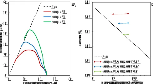
Figure 4-21 comparing S-N cyclic resistance curve of experiment with Artificial S-N resistance curve of simulation in terms of original and modified parameters set. ... 83

Figure 4-22 comparison of initial and modified intergranular parameters in reproducing the stiffness degradation curve ... 83

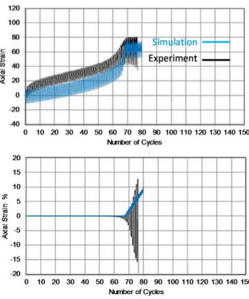
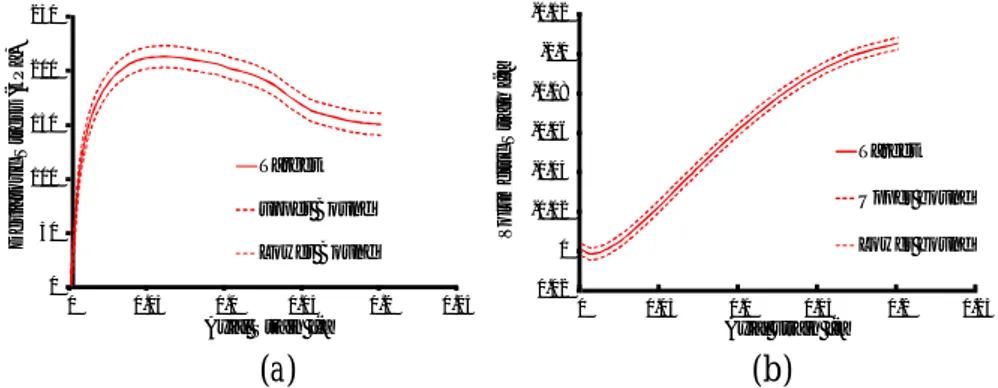
Figure 4-23 Simulation of CTXL5 using the calibrated parameters of the hypoplastic model... 84

Figure 4-24 Simulation of CTXL8 using the calibrated parameters of the hypoplastic model... 85

Figure 4-25 Results of strain-controlled CIU triaxial tests: a) effective stress paths, b) state diagram (data from Eckersley, 1990)... 86

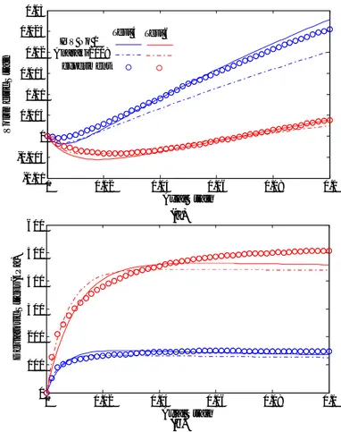
Figure 4-26, Simulations versus observations of CIU tests. ... 89

Figure 4-27, Performance of adopted ISG parameters a) simulation of stiffness degradation curve for Test NP-2 . b) Simulation of Cyclic triaixl test with low deviatoric stress ratio (q/p’ = 0.1)... 91

Figure 5-1, Grain size distribution of the # 2Q-ROK sand ... 96

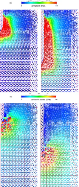
Figure 5-5 Experiment output for Jacked pile installation ( [110]) ... 99 Figure 5-6 CPT results and observations used to calibrate the soil model ... 100 Figure 5-7, Triaxial tests on samples extracted from borehole BH-WFS2-5 ( [101]). ... 101 Figure 5-8, Scheme of the MPM model of CPT... 103 Figure 5-9, Results of the MPM model at penetration depths 2D and 6D: a) deviatoric strain; b) deviatoric stress ... 105 Figure 5-10, Results of the parametric analysis: cone resistance pressure vs. dimensionless depth. ... 107 Figure 5-11, Parameter values during the regression analysis when it is conduced to calibrate on one parameter at the time: a) soil stiffness, E; b) friction angle, f. ... 110 Figure 5-12, Parameter values during the regression analysis when it is conduced to calibrate both parameters simultaneously: a) soil stiffness, E; b) friction angle, f. ... 110 Figure 5-13, Error function during the regression analysis when it is conduced to calibrate parameters E and f simultaneously. ... 111 Figure 5-14, Cone resistance profile with depth for the initial and optimal values of the input parameters in the regression analysis conducted to calibrate parameters E and f simultaneously. ... 111 Figure 5-15 Discretization mesh used in the MPM model of the CPT 113 Figure 5-16 Effect of the mesh size on the model output ... 113 Figure 5-17, simulation of CPT on the loose sample... 115 Figure 5-18, Simulated tip resistance over the iterations ... 117 Figure 5-19, a) relation between volumetric strain and deviatoric strain in the case of two sets of parameters b) deviatoric strain around the cone and shaft after 20 cm of penetration. ... 118 Figure 5-20, Model error function over the iterations. ... 118 Figure 5-21, Horizontal displacement of particle at the depth of 20 cm. a) starting value b) optimal model ... 119 Figure 5-22, Model for simulation of CPT in layered soil, loose over dense layer ... 120 Figure 5-23, Simulation of the CPT on the layered sample, T1LOD, loose over dense ... 121

Figure 5-24, Instability while using MPM-MIXED integration method ... 123 Figure 5-25, Simulation of CPT using MPM-MP+GP and initial parameters value. a) Loose sample b) dense sample ... 124 Figure 5-26, Calibration of the hardening soil model with CPT using modified dilation angles and fine mesh a) Loose sample b) Dense Sample ... 125 Figure 5-27, Simulation of CPT on the layered sample using hardening soil model... 126 Figure 5-28, MPM model for centrifuge experiment of pile installation a) initial stress using K0 Procedure b) stress initialization using the gravity acceleration equal to 40g . ... 127 Figure 5-29, Effect of intergranular parameters on the vertical effective stress of the soil domain while pile is 18 cm penetrated a) suggested IGS parameters b) IGS parameters value suggested by Wegener and Herle (2013)... 128 Figure 5-30 Outcome of MPM model adopting INV02 for hypoplastic main parameters and suggested IGS parameters ( [59]) ... 129 Figure 5-31 Outcome of the modified set of parameter ... 130 Figure 5-32 Vertical effective stress when the pile is 18 cm penetrated. a) Parameters of INV02 b) Modified parameter (hs=100mPa) ... 131 Figure 5-33 Simulation of lab tests using modified parameters, a) oedometer test, b) triaxial tests of INV02 in Chapter 3 ... 132 Figure 5-34 Scheme of the MPM model of CPT. ... 134 Figure 5-35 Comparison between CPT data and computed tip resistance for initial and calibrated values of the input parameters... 136 Figure 5-36 Results of regression at each iteration: values of parameters and objective function. ... 137 Figure 5-37 MPM results: direction of horizontal and vertical displacement at end of penetration for the initial (a) and calibrated models (b). ... 139 Figure 5-38 Comparison between experimental data from triaxial tests and hypoplastic model results for the initial and calibrated values of the input parameters. ... 140 Figure 5-39 Comparison between CPT observations and computed tip resistance for the 5 simulations of the parametric analysis ... 141 Figure 6-1 Schematic of the flume used for propagation tests of granular flows [121]. ... 143

Figure 6-3 Observations, at time equal to 1.5 s, along the longitudinal cross-section of the flume used to calibrate the MPM model. ... 145 Figure 6-4 Scheme of computational domain. ... 146 Figure 6-5 Experimental observations and results of the initial MPM simulation at the end of the test. ... 146 Figure 6-6 Result of model calibration by regression using observations at time t = 1.5 s. ... 150 Figure 6-7 Comparison between model results and experimental observations. ... 151 Figure 6-8 Results of flume test #7 (from Eckersley, 1990): failure and post-failure stages. ... 154 Figure 6-9, MPM model and its initial condition, with the indication of the (moving) tracking points (P1-P5) and the (fixed) control Zones (1-3). ... 155 Figure 6-10, Displacements and deviatoric shear strains computed at different times depending on the initial void ratio. In the Zone 1, at t=0, ep: 0.51 (a), 0.55 (b), 0.61 (c)... 156 Figure 6-11, Displacements and deviatoric shear strains computed at different times for: a) a= 0.34 (original set of parameters) b) a= 0.10 (modified set of parameters). ... 158 Figure 6-12 , Effect of Parameter a on mobilized friction angle. ... 158 Figure 6-13, Evolution of the control points (P1-P5) in the e-p’ plot during the slope instability process. ... 159 Figure 6-14, Mean effective stresses during the three slope instability stages ... 161 Figure 6-15, Pore water pressure and mean effective stress simulated over time at the tracked zones. ... 162 Figure 6-16, Point P1 tracked over time: a) current and critical void ratios; b) mean effective stress... 162 Figure 7-1 (a) Plan view of landslide of topography contours of debris thickness (b) Landslide debris in plan and section views ... 166 Figure 7-2 Typical stratigraphy through the landslide site ( [122]) ... 166 Figure 7-3 Hourly rainfall intensities from 11 to 13 August 1995 ( [122]) ... 167 Figure 7-4 Probable sequence of the events ( [122]) ... 168

Figure 7-5 Groundwater regime ( [122]) ... 169 Figure 7-6 Geological cross section of the slope before that landslide occurred ( [122]) ... 170 Figure 7-7 Direct shear test results for altered tuff with kaolinite veins (a) and for weathered volcanic joints (b) ( [122]). ... 171 Figure 7-8 Water retention curves ( [125]) ... 172 Figure 7-9 Procedure employed to calibrate the input parameters of a numerical model that simulates the propagation of a landslide... 176 Figure 7-10 Location of the landslide deposition height observations used to compute the objective functions for model calibration: a) plan view (modified from [122]); b) cross-section. ... 178 Figure 7-11 Parametric study 1: comparison between observations and computed results for observation set 1 (a) and observation set 2 (b).... 181 Figure 7-12 Parametric study 1: model error variance vs. value of model parameter, tan fb, for the 13 observation sets employed in the analysis.

... 182 Figure 7-13 Step 1 optimization analysis: value of model parameter (a) and model error variance (b) at each iteration of performed regression. ... 185 Figure 7-14 Parametric study 2: comparison between observation set 1 and computed results for three values of model parameter tan fb and

five values of model parameter cv. ... 189

Figure 7-15 Parametric study 2: model error variance vs. value of model parameters, tan f_b and c_v, for observation sets 01 (a), 12 (b) and 13 (c). ... 190 Figure 7-16 Parametric studies 3 and 4: (a) comparison between observation set 1 and computed results considering tan fb = 0.55 and

five values of model parameters pwrel and hwrel; (b) model error variance

vs. values of model parameters for observation set 1. ... 191 Figure 7-17 Values of calibrated parameters and model error variance at each iteration of the regression: (a) calibration of parameter tan fb; (b)

calibration of parameters tan fb and pwrel. ... 192

Figure 7-18 Soil height contour lines for the best-fit parameter estimates: (a) calibration of parameter tanfb; (b) calibration of parameters tan fb

and pwrel. ... 193

Figure 7-21, (a) Critical slip surface at failure time; (b) Suction distribution at failure time ... 197 Figure 7-22, (a) Calculation mesh for the MPM analysis; (b) Geometry of the slope for the MPM simulations. ... 198 Figure 7-23, Deviatoric strain distribution for three simulations with different cohesion values ... 200 Figure 7-24, comparison of the outcome of case 3 with final the geometry of landslide ... 201 Figure 7-25 Results of the inverse analysis ... 202 Figure 7-26, optimal model obtained through the inverse analysis and comparison with initial one. ... 203 Figure 7-27, comparison of the optimal model with final geometry of landslide ... 203

LIST OF TABLES

Table 3-1, Hardening-Soil input parameters ... 46

Table 3-2, Possible range of parameters of Hypoplastic model, suggested by [91]. ... 51

Table 4-1. Triaxial tests used for model calibration. ... 61

Table 4-2 Inverse analyses performed ... 63

Table 4-3 Calibrated parameters compared to [99]. ... 63

Table 4-4 Calibration stages along with adopted observations, variable parameter and method of parameters determination ... 72

Table 4-5 Considered range for main parameters and outcome of calibration in stage 3... 74

Table 4-6 Considered range for intergranular parameters and outcome of calibration in stage 4... 77

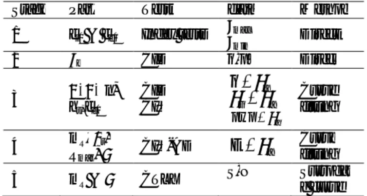
Table 4-7, qualitative sensitivity of the CTXL test to the hypoplastic model parameters ... 81

Table 4-8 Final calibrated parameters of the hypoplastic model for Kreftenheye sand. ... 84

Table 4-9, Estimated values of the parameters for the hypoplastic constitutive model. ... 89

Table 5-1 Summary of studies for CPT modelling ... 94

Table 5-2, the chamber tests on the #2Q-ROK ( [109]). ... 95

Table 5-3 Triaxial tests on samples extracted from borehole BH-WFS2-5. ... 100

Table 5-4 Input parameter values of the parametric analysis ... 104

Table 5-5, Main statistical indicators of the sensitivity analysis ... 108

Table 5-6 Size of elements in discretization mesh used in the MPM Mohr-Coulomb of the CPT ... 112

Table 5-7 Values of the calibrated parameters at each iteration of the regression. ... 117

Table 5-8, Estimated parameters value of hardening soil model based on [85]. ... 122

analysis ... 140 Table 6-1 Composite scaled sensitivities of the model input parameters ... 148 Table 7-1 Soil materials properties (data from [122])... 171 Table 7-2 Sets of observations used for model calibration. ... 177 Table 7-3 Material schematization, rheological laws, values of the input parameters and number of simulations performed for the parametric analyses... 180 Table 7-4 Linear correlation coefficients between the parameters of the rheological law, computed from the variance-covariance matrix for the following values of the parameters: ... 180 Table 7-5, Seepage and slope analyses inputs... 196 Table 7-6, Iinitial input parameters in the MPM simulation of the slope ... 199

AKNOWLEDGMENT

I was not able to carry this research unless with great support, sympathy and patience of my advisors Prof. Sabatino Cuomo and Prof. Michele Calvello who managed well three years of my career. I should also admit that what I achieved in my PhD was not possible without help, support and doctorine of my external supervisor Dr. Mario Martinelli. I also should be grateful to be partially supervised by Dr. Vahid Galavi who transferred lots of knowledge and ideas to me.

I did not find enough words to appreciate the favors of Prof. Settimio Ferlisi in all aspects of my life during these three and half years of PhD.

I also thank the chair of Geotechnical lab of University of Salerno, Prof. Leonardo Cascini, the head of international exchange office of civil engineering department Prof. Salvatore Barba as well as the head of the doctoral school, Dr. Giovani Salzano and the Deltares managers; Harm Aantjes, Dr. Ahmed Elkadi and Ipo Ritesma for their kind favors, supports and allowing me to fulfil my research in their teams and organizations. I would like to acknowledge also Prof. Majid Hassanizadeh from Utrecht Universities for his consultancy and help. I would like to appreciate the patience and support of my new colleagues particularly Professor Tobias Mörz and Dr. Majid Goodarzi in Marum.

I would like to show gratitude to my friends in Salerno , such as my Best friend Dr. Gaetano Pecoraro who has been always beside of me in both happy and sad moments, from the beginning of my stay in Italy till last min. As a foreign student in south of Italy, I am very happy to find great friends in Unisa Geotechnical Lab such as Dr. Dario Peduto, Antonio Marchese, Maria Grazia Stoppiello, , Maria Rosaria Scoppettuolo, Angela Di Perna, Mariantonia Santoro and Dr. Gianfranco Nicodemo, Dr. Luca Picullo , Dr. Vittoria Capobianco, Dr. Ilaria Redina and Dr. Mariagiovanna Moscariello, Ing. Vitto Foresta, Ing. Mauro Forte, as well as my close friends in salerno, Ing. Francesco Montone and Hannes Amberger who always helped me and my wife in various aspects of our stay in Italy.

I also thank my friends and colleagues in Deltares and Anura 3D research comunity to make a great memory for me during those 9 months stay in the Netherland. Thanks to Dr. Alex Rohe, Dr. Francesca Ceccato and Dr. Faraz Sadeghi Tehrani for their consultancy, thanks to Dirk De Lange, Mike Woning, Thomas Bles, Dr. Margareet Van Marle, Wie Lee Lin and Sara Faghigh Naini.

I would like to express my gratitude to the family of Ferullo and especially ’’ il mio padrino Ettore e’ la mia madrina Rosa Desiderio” who always take care of me and my wife like our parents. At the end, I wish to thanks my wife for her perseverance, support and help during these years.

Large deformation analysis has become recently centre of attraction in geotechnical design. It is used to predict geotechnical boundary value problems such as, excessive movement of soil masses like landslides or soil-structure interaction like pile installations. Wrong understanding and simulation of each mentioned problem could lead to significant costs and damages, therefore, robust approaches of modelling are needed. Throughout the past decades many numerical methods aiming to simulate large deformations have been introduced as for example, Discrete Element Method (DEM), Smooth Particle Hydrodynamics (SPH), Updated Lagrangian Finite Element Method (UL-FEM) and Material Point Method (MPM). They are varying in basic theories, capabilities and accuracy. But, the complexity is the feature which is quite common in all them and it is attributed to the unclear response of soil body under excessive deformations. As a result these methods are involving many uncertainties in input parameters. Determination of these parameters is always difficult, because reproducing larg deformations in the laboratory is difficult and needs advanced and expensive facilities. As a result the introduction of a methodology for estimation of the model parameters adopted for large deformation analysis is extremely needed.

Inverse analysis approaches have proved to be able to overcome complex engineering problem in different fields. In geotechnical engineering, inverse analysis is typically employed to back-calculate the input parameter set of a model to best reproduce monitored observations. Accordingly, its application attempts to clarify the effective soil conditions and allows for an update of the design based on the in-situ measurements. Numerous researches have been fulfilled to evaluate the performance of this approach in geotechnical problem, however, rarely the application of this methodology to the problems involving large deformations have been addressed.

This thesis is addressing these issues by combining inverse analysis methods with advanced numerical methods and soil constitutive models. The proposed methodology is applied to two popular large deformation engineering problem i.e. landslides and soil-structure interaction,

particularly cone penetration tests modelling. Different case studies are addressed; two methods of Smoothed Particle Hydrodynamic and Material Point Method are adopted as numerical models, depending on the case study. Similarly, various constitutive models ranging from the simple Mohr-Coulomb to the advanced ones such as Hardening soil and Hypoplastic model are employed. The employed inverse analysis algorithm also varies by the type of the numerical models and required computation time of the forward model. Particularly, two algorithm are selected, a gradient-based method (modified Gauss-Newton method) and an evaluation based one (Species- based Quantum Particle Swarm Optimization).

In each case the strength and shortcoming of the adopted methods as well as the role played by the adopted benchmarks and the type of observation in model calibration is assessed. A concept of in-situ recalibration of the model is defined and its importance is highlighted. This method is used to determine advanced constitutive model parameters using in-situ tests and geometrical observations.

As a conclusion, the research shows how using an inverse analysis algorithm may improve the modelling of geotechnical problems involving large deformations and, particularly, facilitate model calibration and discovering the shortcoming and strength of the numerical models.

Pooyan Ghasemi earned a Master of Science in Seismic Geotechnical Engineering at the University of Tehran (Iran) in 2012 with a dissertation on "Experimental study of remediation measures of anchored sheet pile quay walls using soil compaction". He conducted experimental (shaking table test) and numerical (Finite Element Method) investigation on the remediation measures of anchored sheet pile quay walls that are embedded in the liquefaction-susceptible soil. After his master degree, he started working in Hexa consulting Engineer Company where he has gained some professional experiences in designing of roadways and railways infrastructures such as bridges, tunnels, retaining walls, etc. Since December 2015, he was awarded a PhD position by the Laboratory of Geotechnical Engineering at University of Salerno. Meanwhile, he has been also a visiting scholar at Deltares (The Netherlands) for almost 9 months working on applications of the material point method to geotechnical problems and on the implementation of inverse analysis algorithms in the MPM code. He also was partially involved in JIP-SIMON project, a Joint Industry Project on the Simulation of installation of offshore Monopile. During the PhD and mentioned project, he earned valuable skills in program developing, advanced numerical methods, Constitutive models, and laboratory and in-situ tests data interpretations.

By the time of finalizing his PhD, he has joined MARUM, Centre for Marine Environmental Science, Bremen-Germany, in order to work within a research project about offshore wind turbine foundations.

Soil characterization and estimation is the first step in geotechnical design and engineering. It is not exaggerating if one says the core of geotechnical engineering is site characterisation. Because, proper, certain and accurate determination of the soil properties leads to the efficient design and subsequently significant cost reduction. On the other hand recent design approaches are highly coupled with risk assessment and mitigation which requires a reliable prediction of site or nature response to the human or atmospheric induced disturbance. Such predictions could be carried out through the numerical modelling.

Many geotechnical problems involve large deformation and large movement of soil mass. As examples of such problems, landslides and pile driving could be quoted. The analysis of such a problem is challenging, and need to be simulated using numerical methods developed for large deformation modelling. To name few, the Arbitrary Langrangian Eulerian Finite Element Method (ALE), the Coupled Eulerian-Lagrangian (CEL) or particle-based methods such as Smoothed Particle Hydrodynamics (SPH) or Material Point Method (MPM). They are varying in basic theories, capabilities and accuracy. But, the complexity is the feature which is quite common in all them and it is attributed to the unclear response of soil body under excessive deformations. As a result these methods are involving many uncertainties in input parameters. Determination of these parameters is always difficult. Moreover, in order to simulate the elaborated circumstances, adopting the advanced numerical method is needed. Advanced numerical methods which usually involve a large number of parameters mostly need to be coupled with soil advanced constitutive model able to reproduce soil hydro-mechanical behaviour properly. However, difficulties in determination of both numerical and constitutive parameters might undermine the practicability of advanced numerical models. Therefore, many engineers still are willing to rely on the empirical methods to predict the geotechnical problem whilst those methods are not enough accurate in many cases.

In the thesis, an attempt has been carried out to first of all show how the inverse analysis technique could be used to determine the soil constitutive and numerical parameters. Secondly, a comprehensive methodology on the application of inverse analysis to the landslide flow slide in both failure and propagation stage is proposed. In addition, a novel methodology is going to be presented by which the soil parameters of advanced constitutive models could be determined based on the results of laboratory and in-situ tests (cone penetration tests) while adopting inverse analysis technique. The benefit, challenges and drawbacks of adopted methodology would be discussed.

To reach the aforementioned aims, the needs of a robust method to large deformation modelling are indisputable. Accordingly, two recently developed numerical methods adopted for large deformation phenomenon have been addressed: 1) SPH, which has been used to simulated the propagation stage of a landslide case study, 2) Material point method, which is a novel robust numerical approach able to cover both failure and large strain of the material. In this thesis, MPM has been used to simulate two different geotechnical problems, 1) flow-like landslide case studies covering the initiation of failure until end of the propagation, 2) Simulation of Cone Penetration Tests (CPTs) in sandy soils.

1.1 LAYOUT OF THE THESIS

The second chapter consists of a brief literature review on the application of inverse analysis approach in geotechnical problems. In addition, the chapter presents a brief review on the studies fulfilled on the numerical simulation of the geotechnical problems addressed in theses thesis, i.e. retrogressive failure and flow-like landslide in a slope, landslide propagation and also simulation of cone penetration tests. In the third chapter, the material and methods used in this study are introduced, starting from the ingredients of inverse analysis including the error definitions and optimization algorithms. Then, the adopted numerical methods i.e. the Material Point Method (MPM), Smoothed Particles Hydrodynamic (SPH), are described. In addition, the three adopted constitutive models in this study are discussed. At the end, a general framework in order to apply inverse analysis to landslide soil

characterisation through the usage of various numerical methods is introduced.

In the fourth chapter, the automatic parameter estimation of advanced constitutive model using REV and lab data is presented, proposed method is applied to estimate the hypoplastic constitutive model in terms of three different cohesion-less material. The adopted laboratory data includes both cyclic and monotonic tests

The fifth chapter of this study is devoted to the in-situ soil parameters estimation through the application of inverse analysis to the material point method model of cone penetration tests. First, the feasibility of the method would be checked by employing a simple constitutive model. Then, the methodology is applied to two advanced constitutive models. The benefit and shortcomings of the method would be discussed.

In the sixth chapter, the automated inverse analysis procedures are used to calibrate the MPM models of two well-instrumented laboratory experiments on reduced-scale slopes, respectively dealing with (1) long run-out soil propagation and (2) large slope deformation. The first laboratory test reproduces a soil mass rapidly propagating along an inclined plane and depositing over a flat area. The second test refers to a retrogressive slope instability combined with soil liquefaction.

In the seventh chapter, a real rainfall induced landslide is addressed. The framework introduced in the last section of chapter 3 is adopted to combine the inverse analysis algorithm with three different numerical methods of LEM, SPH, and MPM. At the end the hydraulical and mechanical parameters of the soil which leads to the best reproductions of landslide triggering and propagation stage are estimated and reported.

In this chapter some of the studies related to geotechnical problems addressed in this thesis are reviewed. The studies are presented in three different sections. First, the state of art related to the applications of inverse analysis to the geotechnical problem is presented.

Two main geotechnical problems of this study are the landslides and the Cone Penetration Tests (CPT). The literature on these two topics is widely extended. Therefore, just few studies related to the simulation of these two problems are discussed here. In the Sec. 2.2 a summary of studies related to the simulation of flow slides and retrogressive failure is discussed. In Sec.2.3 a brief literature review on the simulation of penetration problems using different numerical method is performed.

2.1 INVERSE ANALYSIS AND THE

GEOTECHNICAL PROBLEMS

[1] presented one of the first geotechnical back-analysis, where the identification of rock mass parameters during a tunnel excavation was carried out. The least squares criterion was used to define the objective function, while a direct method was applied to minimize it.

In [2] and [3], back-analyses applied to earth dam problems were studied. Subsequently, [4] presented some remarks on back-analysis and characterization problems in geomechanics.

Simultaneously to the trend initiated by [4], a Japanese group (formed by the universities of Kobe, Kyoto and Tokyo) was strongly working on the field of back-analysis applied to geotechnics. Several back-analyses for tunnel excavations were performed by [5] and [6], as well as for consolidation and test embankments on soft clay deposits in [7].

Since the advent of numerical methods like Finite Element Method (FEM), the adaptation of the back-analysis in geotechnical problem become more popular, the methodology was applied to different problems to determine various kind of model input parameters from soil mechanical properties to hydraulic parameters. In addition different kinds of observation regarding the objective problem were employed. Having a general view on the literature implies that, as the models are getting more complicated, tend to use automatic calibration rather than conventional back-analysis has increased.

In the geotechnical community, always there is a distinction between the soil behaviour in lab and field condition. Traditionally, soil parameters have been obtained from laboratory tests. However, in many cases samples used in laboratory tests do not represent the whole soil profile. In addition to that, sample extraction itself causes some disturbance and changes of the soil properties that are difficult to quantify. This fundamental distinction has also influenced the researches fulfilled using inverse analysis technique so that, the automatic calibration of the parameters could be classified in two groups. 1) Automatic parameter estimation based on lab data. 2) Automatic parameter estimation based on the field data. Obviously, these two categories are altered in the model being used to simulate the objective data. The former consists in single element or constitutive modelling while the latter is involving a boundary value problem modelling.

As for the first group of mentioned research, the main benefit of inverse analysis technique rises when dealing with an advanced constitutive model involving large number of input parameters. For example, many researchers have been carried out using different approach of inverse engineering to determine the parameters of cam clay. [8] calibrated the model using Modified Guass Newton Method. The model parameters also estimated using lab data and neutral network by [9], [10] identified the cam clay model parameters using lab data and particle swarm optimization method (PSO). Obviously, automatic parameters estimation for simple constitutive model with little number of parameters based on lab data does not worth hassling like Mohr-coulomb model in which the parameters can be estimated based on the interpretation of the lab data and the executing of the model and iterative procedure is not needed. In the second category of application (Application to the boundary value problem), the aim is to estimate the soil parameters for in-situ condition and find the optimal value of parameters which yields the best matches between model and real field data. In this category, the application even to the simple constitutive model is very beneficial because, even the estimation of in-situ parameters for simple model is not an easy tasks. In the previous studies, many researches focused on application of inverse analysis to the excavation such as [11]in which the parameters were estimated from inclinometer data, [12] discussed the advantages and disadvantages of using genetic algorithms and self-learning simulations for inverse analysis in a deep urban excavation. Finally, in [13], a simple synthetic tunnel excavation was used to illustrate the potential of the hybrid methodology to parameter estimation.

In addition to the excavation, back-analysis and inverse engineering have been always employed in slope stability and landslide studies. The previous studies mainly devoted to determine the soil parameters by back-analysing of the failure surface and factor of safety. Started by [14] and then followed by [15] who used the pore water pressure information to back-analysis of landslide. [16] for the first time encountered the high correlation of the parameters and admitted the different combination of C and phi may lead to similar failure surface.

Inverse modelling has been employed for different slope stability and landslide study ( [17] [18]; [19]; [20]). The majority of the research conducted on this topic has focused on landslide triggering employing the hydraulic response of the slope, such as measures from piezometers, as observations to identify the model soil properties ( [21]; [22].

Landslide propagation behaviour, although a subject of broad and current interest (e.g., [23]; [24]; [25]), has rarely been coupled with inverse analysis algorithms explicitly considering the geometric characteristics of the slope as observation values, which may include ground displacements and run-out soil heights (e.g., [26]). This kind of data is particularly useful for the simulation of the propagation stage of landslides. Concerning that, for a well-posed inverse analysis problem, it is very important to choose proper sets of observations - not always an easy task to perform. The propagation stage modelling of a landslide requires a numerical model capable to simulate large deformations. Since such these methods are becoming more popular and developed. Investigation on the practicality of inverse analysis methods to calibrate these models are required .

Large deformation numerical methods also provided the possibility of the penetration problem modelling like cone penetration tests or pile driving ( [27], [28]and [29]). This gives a good opportunity to estimate the in-situ soil parameters using the data recorded during penetration process. [30] shows that adopting inverse analysis helps to overcome the complexity of the soil-density and strength relation in field condition. As it was mentioned, the inverse analysis has been applied in many research to estimate the soil parameters either using field data or laboratory testing data. But, rarely the parameter estimation using simultaneously are both types investigated. In this case, the real influence, robustness, performance and shortcoming of the model remain unknown. This researches aims to advertise the inverse analysis approach not only as a tool to back-analysis of a phenomenon, but also a useful tool for prediction and future design. Thus, in the scope of this thesis, a general overview to both lab data and the corresponding field data is addressed with particular attention to the boundary value problems involving large deformations.

2.2 ANALYSIS AND SIMULATION OF FLOW-LIKE

LANDSLIDES

Rainfall-induced instability mechanisms of real and reduced-scale slopes may consist in development of successive shear bands, progressive or

retrogressive landslides induced by (or causing) soil static liquefaction, associated to large deformations of soil. Slope geometry, and the initial and boundary conditions within a slope are key factors for these processes [31]. Flume tests performed on reduced-size slope models provided pioneering measurements of the build-up of pore water pressure after slope failure [32]. Such tests were later extended to complex groundwater conditions, including infiltration from ground surface and/or a downwards/upwards water spring from the bedrock to the tested soil layer [33]. On the other hand, centrifuge tests on artificial-real-size slopes pointed out that the transition from slide to flow is caused by local failures producing a variation in the slope geometry [34]. This mechanism is related to transient localized pore-water pressures that are not associated to the development of undrained conditions, but originated by contrast in soils’ permeability, combination of particular hydraulic boundary conditions and stratigraphical settings. Experimental evidences show that the transition from slide to flow can occur both for loose and dense soils. Even, decreasing pore-water pressures were measured during the post-failure stage due to soil large deformations and soil volume increase [35]; [36].

The evolution of pore water pressure and shear strength mobilized upon deformation, the transition from slide to flow, and the post-failure build-up of pore water pressure depend on the soil constitutive behaviour. Laboratory tests performed on REV (Representative Elementary Volume) proved that instability and failure are two different behaviours of soils that exhibit non-associated flow rule [37]. Although both may lead to catastrophic events, they are not synonymous. In loose fine sands and silts with relatively low permeability, a small disturbance in load or even small amounts of volumetric creep may produce undrained conditions, and consequently instability of the soil mass. As long as the soil remains drained, it will remain stable in the region of potential instability. In particular, in very loose cohesionless materials the excess pore water pressure may increase immediately and cause the effective stress to drop rapidly leading to soil liquefaction [38]. The development of total or partial undrained conditions upon shearing is the main cause of high pore-water pressures, as observed in REV laboratory tests such as consolidated isotropically undrained triaxial tests (CIU), consolidated anisotropically undrained triaxial tests (CAU), constant shear drained triaxial tests (CSD). The build-up of pore pressures is relevant for soils

having low density index, fine grain size, low hydraulic conductivity and subjected to high deformation rate, as reviewed by [31].

Accurate simulation of soil behaviour requires necessarily advanced constitutive models. However, model calibration is neither easy, as the parameters are generally several, nor objective, as calibration is usually based on expert-judgement. This is an open issue, especially for slope stability.

On the other hand, the analysis of slope behaviour can be conducted through a variety of approaches, considering slope geometric configuration, soil behaviour and specific triggering factors and mechanisms. [39] showed that the drained failure of shallow covers subjected to rainfall can be satisfactorily simulated by either well-known Limit Equilibrium Methods (LEMs) [40]; or more sophisticated Finite Element Method (FEM) analyses [41]. The accurate simulation of both pore water pressure evolution and increase in strain rate necessarily requires advanced constitutive model, such as the Generalized Plasticity model [31]. In such cases deformations are either neglected (LEM) or generally considered as "small" (FEM), which may be a reasonable hypothesis when pre-failure and failure are the only issues of the analysis. The simulation of the overall evolution of slope geometry and the related large deformations requires other approaches such as extended versions of FEM (e.g. Finite Element Method with Lagrangian Integration Points, FEMLIP, [42]; [43], meshless methods such as Smooth Particle Hydrodynamics (SPH, e.g. [44]; [45], or other methods like DEM (Discrete Element Method; e.g. [46]).

The Material Point Method (MPM) was recently used to simulate: progressive failure of river levees [47]; retrogressive and progressive slope failures induced by excavation [48]; progressive failure and post-failure behaviour for a deep-seated rockslide with a similar geometry to Vajont landslide [49]; dam break flows with different initial aspect ratios [50]; and landslide propagation [51]. However, the literature still lacks contributions which combine MPM slope simulation, the use of advanced soil constitutive model and the calibration of the model by inverse analysis and some recent contributions were recently proposed.

2.3 SIMULATION OF PENETRATION PROBLEMS

The numerical simulation of cone penetration tests (CPT) is always a hot topic for large deformation numerical studies. The majority of the research investigated on the simulation of CPT tests in the cohesive material (Clay). Fully undrained or partially drained condition are expected for these material. In saturated clays and other fine-grained soils, the test is carried out at a penetration rate that does not permit drainage, therefore the cone resistance may be interpreted as a measure of the undrained shear strength of the soil. Some of the valuable studies on the numerical modelling of CPT in clayey material are as follows; [52] adopted the ALE method with 4-noded interface elements at the soil-cone contact. He carried out undrained total stress analyses with Tresca material model. He considered the effects of the soil stiffness, the roughness of the cone and the initial stress state. [53] adopted the CEL method to simulate cone penetration in clay.

[54]compared the performance three numerical analysis approaches capable of accounting for large deformations in simulation of cone penetration tests. They compared the implicit re-meshing and interpolation technique by small strain (RITSS), an efficient Arbitrary Lagrangian–Eulerian (EALE) implicit method and the Coupled Eulerian–Lagrangian (CEL). In all the cases,. Clayey soils rather than sands were explored, allowing focus on comparison of the performance of the three numerical approaches without the additional complication of a constitutive relationship that appropriately captures the behaviour of sandy soils. It was concluded that the three methods yield similar results for the quasi-static penetration problems. In the CEL analysis the penetration velocity and critical time step need to be selected carefully, while the re-meshing interval requires attention in the two selected implicit methods. the result obtained with the CEL show dependency on element size (even very fine mesh was used in the region concerned) and differs from those predicted with the EALE and RITSS. The exact solution for this problem is not known.

[55] employed the implicit quasi-static MPM formulation with 3-noded triangular interface elements to perform undrained total and effective stress analysis of cone penetration. His results are in good agreement with those of van den [52] and [56] [57] repeated the same study using explicit time integration scheme MPM formulation.

The simulation of penetration in sandy soils seems to be more challenging. On one side, the instability of the model regarding the absence of the cohesion is more likely; secondly, the shear strength of sand requires more complicated failure criterion rather than those of Tresca model.

Accurate numerical modelling of cone penetration in sand requires a constitutive model that captures stress- and state-dependent response of the soil. [58]shows that the use of a very complex constitutive model to realistically simulate cone penetration in sand can be extremely challenging, keeping in mind that the problem involves high mesh distortion and frictional con tact in finite element analysis.

[27] also evaluates the effect of analysis parameter choices on the stability and efficiency of modelling cone penetration into sand

Since the material point method shows acceptable performance in simulation of cone penetration test in Clay [55] and [57], [29] adopted this method to simulate a jacked pile installation in sand. The study clearly shows the challenges in input parameters and necessity to recalibration of the soil constitutive model parameters.

A big challenge in the adopted MPM model by Phuong was the high computation times for simulation few centimetre penetrations. That was due to the fact that, they adopted a 3D MPM formulation. Then, [59] presented axisymmetric MPM formulation which reduced significantly the required computational time.

In this study the axisymmetric MPM model of [59] would be employed to simulate the cone penetration tests in sandy soil, since the computation times are expected to be less than previous models, this thesis can focus on the challenges and performance of constitutive model for CPT modelling in sand and the parameter estimation as well, which is quite missing in the previous researches.

In this chapter, the materials and methodology used in this thesis are presented. Sec.3.1 describes the inverse analysis concepts in details. Its ingredients and elements along with their alternatives to be employed are discussed. It would be explained the main elements of the algorithm are Forward model (herein the numerical methods and constitutive models), error definition and optimization methods. Thus, as for the forward model, Sec. 3.2 is devoted to explain the material point method concept and its formulation for two phase material and one phase in axisymmetric condition. In addition, another numerical method adopted in this thesis (Smoothed Particles Hydrodynamic) is briefly presented in Sec.3.4

Sec.3.3 explains the constitutive models employed in various context of this thesis, a simple model of Mohr-Coulomb, Hardening Soil as a semi complex model and Hypoplastic model as a complex model. The strength and weakness of each model along with their difficulties to be used in material point method formulation are also discussed

At the end of this chapter, a framework would be proposed by which the inverse analysis is applied to a rainfall induced landslide. One can use this framework to combine three different models of LEM (Limit Equilibrium Method), SPH and MPM to determine the soil hydromechanical properties and calibrate the models

3.1 INVERSE ANALYSIS ALGORITHMS

Inverse analysis consists in an iterative procedure to estimate the model input that produces the closest output to the user expectation. In other words, an inverse analysis algorithm is searching a set of input parameters that makes the minimum possible difference between the model outcome and the observations. These differences may be called the error, model error function, or objective function. Thus, the best input of the forward model is the one that minimizes the error function. Optimization problems can be classified based on the type of constraints, nature of design variables, physical structure of the problem, nature of the equations involved, deterministic nature of the variables, permissible value of the design variables, separability of the functions and number of objective functions [60].

Classification based on the existence of constrains

· Constrained optimization problems which are subject to one or more constraints.

· Unconstrained optimization problems in which no constraints exist

Classification based on the nature of the design variables

· Parameter or static optimization problems: the objective is to find a set of design parameters that make a prescribed function of these parameters minimum or maximum subject to certain constraints.

· Trajectory or dynamic optimization problems: the objective is to find a set of design parameters, which are all continuous functions of some other parameter that minimizes an objective function subject to a set of constraints.

Classification based on the physical structure of the problem.

· An optimal control problem is a mathematical programming problem involving a number of stages, where each stage evolves from the preceding stage in a prescribed manner. The problem is to find a set of control or design variables such that the total objective functions over all stages is minimized subject to a set of constraints on the control and state variables.

· The problems which are not optimal control problems are called non-optimal control problems.

Classification based on the nature of the equations involved.

· Linear programming problem: if the objective function and all the constraints are linear functions of the design variables.

· Nonlinear programming problem: if any of the functions among the objectives and constraint functions is nonlinear.

Based on the mentioned type of the problem, the best type of optimization algorithm should be chosen. Apart from the mathematical point of view, the time of the computation becomes a relevant issue when the forward model is a numerical model. In this thesis two different kinds of optimization methods are used for different applications and purposes.

1) When the forward model is not time consuming, such as for the simulation of a single element model, performing a high number of iterations is not an issue, therefore a particle swarm optimization algorithm is used.

2) When the forward model is time consuming, the number of iteration needed to solve the problem must be minimized, therefore a gradient based optimization method is used.

Later in this chapter, the two optimization methods employed in this thesis will be presented and discussed.

3.1.1 Error Definition and Normalization

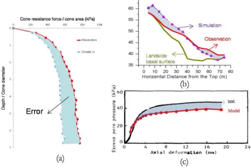
One of the most important elements of inverse analysis is the definition of a proper Model Error Function. Generally, the Model Error Function can be defined as a function reporting the fit between model outcomes and observations. The main inherent feature of all optimization methods is that they use some iterative procedures to minimize the Model Error Function. If we think at the observations as curves, a simple definition of the Model Error Function (MEF) could be the area between the curve representing the simulation and the observed curve. Figure 3-1 illustrates schematically this approach of error definition.

Depend on the employed optimisation algorithm, the Model Error Function could be defined as a vector or as a scalar. Usually gradient based optimization methods are compatible with a vector error based on least squared error quantification approaches. On the other hand, methods like Genetic algorithms of Particle Swarm methods incorporate a scalar error in their formulation.

A challenge in defining a proper Model Error Function arises when the observations to be used vary in type and magnitude. In this case, the errors corresponding to each type of observation should be normalized and properly weighted.

Figure 3-1, Visualization of the error between observations and simulations for different geotechnical problem (a) Cone Penetration Tests (b) Landslide propagation (c) Lab tests.

3.1.1.1 Weighting methods

When different types of observations or observations with significantly different magnitudes are used, the computation of the total error of the

model, quantifying the misfit between simulated and experimental results, necessarily calls for the normalization of the observations.

To overcome the challenge of observations with different units, [8] suggested to normalize the observations by the measurement error of the experiments so as to compute a dimensionless error for each observation. Most of the time, however, the error of the measurements is either not reported or not known. In such a case, the normalization could be performed in terms of the maximum desired mismatch between observations and simulated results.

For example, in the case of drained triaxial tests, usually the following two curves are of interest: deviatoric stress versus axial strain, and volumetric strain versus axial strain. It is possible to define an interval representing an acceptable range of model prediction corresponding to the observations reported in those two planes. To compute a total dimensionless error, the observations could be normalized referring to the width of that interval at each observation point.

Figure 3-2 , Examples of desired error intervals for the results of drained triaxial tests.

The advantages of the mentioned approach are the following, 1) It provides a visual representation of acceptable errors

2) For each considered “curve” each observation can be normalized adopting a different normalization value

3) More emphasis can be attributed to some parts of the curve by using smaller desired error intervals in those parts

(a) (b) 0 50 100 150 200 250 0 0.05 0.1 0.15 0.2 0.25 D e v ia to ri c S tr e s s (k P a ) Axial Strain [-] Target upper Bound Lower Bound -0.12 -0.1 -0.08 -0.06 -0.04 -0.02 0 0.02 0 0.05 0.1 0.15 0.2 0.25 V o lu m e tr ic S tr a in [-] Axial strain [-] Target Upper bound Lower bound

Another challenge in the definition of the error function is related to the different magnitude of the observations. For example, in order to calibrate the parameters of constitutive models using lab tests data, different tests with various initial stress levels are typically carried out. In these cases, since the aim of calibration is to find a set of parameter values that matches all of the tests simultaneously, the errors of each curve must be properly weighted.

3.1.1.2 Error definition of lab data curve fitting

There are different approaches available for weighting the observations to be used in an inverse analysis algorithm. One of them could be the normalization of each experimental curve considering the values of the observations reported in that curve such as, for instance, the minimum, the medium or the maximum value of the considered observations. For example, in order to define the error function to calibrate a series of triaxial tests, the error function (EF) could be defined as the sum of the error functions of each considered experimental curve, EF(k):

1 ( ) N k EF=

å

å

number of observations adopted to define the k-th experimental curve,

ek(i) is the weighted residual related to the i-th observation of the k-th

experimental curve, y_k(i) is the value of the i-th observation of the k-th

experimental curve, y’k(i) is the value computed by the model which

corresponds to the i-th observation of the k-th experimental curve, wk(i)

is the weight assigned to the i-th observation of the k-th experimental curve.

The weights were assigned to produce dimensionless weighed residuals,

ek(i), so that the error functions of the considered experimental curves,

EF. The weight assigned to the i-th observation of the k-th experimental

curve is thus defined as follows:

) ( 1 ) ( i s i w k k = ( 3-4)

If the weights assigned to all the observations of a given experimental curve are equal, i.e. they do not depend on the value of the i-th observation of that curve, the expression used to quantify the acceptable error of the k-th experimental curve, sk, can be the following:

( ) max( )

k k k k

s i =s =r y ( 3-5)

where: rk is the dimensionless tolerance coefficient of the k-th

experimental curve, max(yk) is the maximum observed value of the k-th

experimental curve.

Considering the above relationships, Eq. 1 can be expressed as follows:

2 3 1 1 1 [ ( ) ' ( )] [r max(y )] k m N k k K k k i EF y i y i = = =

å

å

3.1.1.3 Error definition for boundary value problem and scattered observations

When the calibration of a boundary value problem such as the simulation of cone penetration tests or a landslide is of interest, single scattered or non-continue observations need to be employed. Since the single simulation of a numerical boundary problem is usually time consuming, it is typically convenient to adopt a gradient based optimisation algorithm to calibrate the model. Gradient based methods usually work with a squared weighted error function S(b), often called objective function, expressed by:

( )

( )

( )

S b =_ëéy-y b _ûù w_ëéy-y b ù_û=e we ( 3-7) where b is a vector containing values of the number of parameters to be estimated; y is the vector of the observations being matched by the regression; y′(b) is the vector of the computed values which correspond

to observations; w is the weight matrix; and e is the vectors of residuals, i.e. the differences between model prediction and observation.

A commonly used indicator of the overall magnitude of the weighted residuals, which allows a direct comparison of results deriving from inverse analyses employing different sets of observations, is the model error variance, s2_:

= ( )₋ ( 3-8)

where ND is the number of observations, and NP is the number of estimated parameters.

3.1.2 Optimisation Algorithm

There are a number of other issues that affect proper calibration of a numerical model by inverse analysis, including: the number of parameters to be optimized, the interdependence of the model parameters within the framework of the constitutive model, the number of observations, the type of system under consideration, and the adopted optimization algorithm ( [8]). Optimization algorithms can be classified in a variety of ways, for instance differentiating between deterministic and probabilistic algorithms or between gradient-based and derivative-free methods. A recent review of optimization techniques widely used in geotechnical engineering is presented by [61]). [62] showed the capability of Modified Gauss Newton Method as a gradient based method in the geotechnical problem. Among the stochastic techniques, Particle Swarm Optimization (PSO) has been shown to provide valuable results in various inverse geotechnical problems, including parameter identification of constitutive models ( [63]; [64]; [10]; [65]). However, being trapped in the local minima is always a matter when using these two optimization methods. In this thesis, addition to the modified Gauss Newton Method, a modification of PSO which is thought to have less possibility of local minimum (SQPSO) is adopted.

3.1.2.1 Modified Guess Newton Method

In this section a gradient based model calibration algorithm implemented in UCODE 2014 [66], a computer code designed to allow

inverse modelling and parameter estimation problem, would be described. UCODE has initially been developed for ground-water models, but it can be effectively used in geotechnical modelling because it works with any application software that can be executed in batch mode. Its model-independency allows the chosen numerical code to be used as a “closed box” in which modifications only involve model input values. This is an important feature of UCODE, in that it allows one to develop a procedure that can be easily employed in practice and in which the engineer will not be asked to use a particular forward or inversion algorithm. Figure 3-3 shows a detailed flowchart of the parameter optimization algorithm used in UCODE. Note that the minimization requires multiple runs of the Forward model.

Figure 3-3 Parameter optimization algorithm flowchart (modified from [8])

In UCODE the weighted least-squares objective function is used and The modified Gauss-Newton method used by UCODE to update the input parameters is expressed as:

(

)

(

( )

)

FE run Updated results

Perturb bkby user-defined amount FE run Computed results Calculate X_ik=∂y_i/∂bk (for i = 1 to ND) Repeat for k=1 to NP ND = Number of observations NP = Number of parameters to optimize YES Forward Model Run Forward Model Run Forward Model Run Eq. 3.7 Eq. 3.9 & 3.10

where dr is the vector used to update the parameter estimates b; r is the parameter estimation iteration number; Xr is the sensitivity matrix

(Xij=∂yi/∂bj) evaluated at parameter estimate br; C is a diagonal scaling

matrix with elements cjj equal to 1/√(XT_{w X)}

jj; I is the identity matrix; mr

is a parameter used to improve regression performance; and rr is a

damping parameter.

For problems with large residuals and a large degree of nonlinearity, the term XrTw Xr is replaced by XrTw Xr + Rr [67] to help convergence when

the objective function changes less than 0.01 over three regression iterations.

Multiple runs of the forward model are required to update the input parameters at a given iteration because the sensitivity matrix Xr is

computed using a perturbation method. At any iteration every input parameter bk is independently perturbed by a fractional amount to

compute the results’ response to its change. Sensitivities are calculated by forward or central differences approximations. For these approximations each iteration requires (NP+1) and (2NP+1) runs, respectively, to estimate a new set of updated parameters, where NP is the number of parameters optimized simultaneously. Computation time may become an issue for very complicated finite element models, depending on how much time is needed for a single model run.

At a given iteration, after performing the modified Gauss-Newton optimization (( 3-9) and ( 3-10)), UCODE decides whether the updated model is optimized according to two convergence criteria. The parameter estimation is said to converge if either:

i) the maximum parameter change of a given iteration is less than a user-defined percentage of the value of the parameter at the previous iteration;

ii) The objective function, S(b), changes less than a user-defined amount for three consecutive iterations.

When the model is optimized the final set of input parameters is used to run the model one last time and produce final “updated” results.

3.1.2.2 Input parameters statistics

The relative importance of the input parameters being simultaneously estimated can be defined using parameter statistics, including the sensitivity of the predictions to changes in parameters values, the variance-covariance matrix, confidence intervals and coefficients of variation.

Different quantities can be used to evaluate the sensitivity of the predictions to parameters changes. One percent sensitivities, dssij, scaled

sensitivities, ssij, and composite scaled sensitivities, cssj, can be used for

the purpose. These sensitivities are defined in Eq.( 3-11) to ( 3-12), respectively. ' 100 j i ij j b y dss b ¶ = ¶ ( 3-11) 1/ 2 'i ij j ii j y ss b b w æ_¶ ö = ç_ç ÷_÷ ¶ è ø ( 3-12) ( 3-13) 1/ 2 2 1/ 2 1 ' ND i j j ii j j b y css b ND b w = é _{ææ ö ö} ù ¶ ê ú =_ê ç_çç_ç ÷_÷ ÷_{÷ ú} ¶ è ø è ø ê ú ë û

å

where y′i is the ith simulated value; yi/bj is the sensitivity of the ith

simulated value with respect to the jth _{parameter; b}

j is the jth estimated

parameter; wjj is the weight of the ith observation

One percent scaled sensitivities represent the amount that the simulated value would change if the parameter value increased by one percent. Scaled sensitivities are dimensionless quantities that can be used to compare the importance of different observations to the estimation of a single parameter or the importance of different parameters to the calculation of a simulated value. Composite scaled sensitivities indicate the total amount of information provided by the observations for the estimation of one parameter.