A fractional optimal control problem for
maximizing advertising efficiency
∗Igor Bykadorov1, Andrea Ellero2, Stefania Funari2, Elena Moretti2 1Sobolev Institute of Mathematics
Siberian Branch Russian Academy of Sciences Acad. Koptyug avenue 4, 630090 Novosibirsk - Russia
2Dipartimento di Matematica Applicata
Universit`a Ca’ Foscari di Venezia Dorsoduro 3825/E, 30123 Venezia - Italy [email protected], [email protected], [email protected]
November 5, 2007
Abstract
We propose an optimal control problem to model the dynamics of the communication activity of a firm with the aim of maximizing its efficiency. We assume that the advertising effort undertaken by the firm contributes to increase the firm’s goodwill and that the goodwill affects the firm’s sales. The aim is to find the advertising policies in order to maximize the firm’s efficiency index which is computed as the ratio between “outputs” and “inputs” properly weighted; the outputs are represented by the final level of goodwill and by the sales achieved by the firm during the period considered, whereas the inputs are represented by the costs undertaken by the firm, fixed costs and advertising costs. The problem considered is formulated as a fractional optimal control problem. In order to find the optimal advertising policies we use the Dinkelbach’s algorithm, for fractional programming.
Keywords: optimal control, advertising, efficiency, fractional programming.
∗Supported by Universit`a Ca’ Foscari di Venezia, MIUR - PRIN co-financing 2005, and the Council for Grants
1
Introduction
We propose a fractional optimal control problem to model the dynamics of communication activity of a firm with the aim of maximizing its efficiency.
The problem of determining the optimal communication policy undertaken by a firm has been largely analyzed in marketing literature by means of dynamic optimal control models (see Sethi, 1977 [11] and Feichtinger et al., 1994 [5], for a review). The various advertising models essentially differ from each other in the dynamics which connects advertising to sales and in the objectives pursued by the firm.
In this paper we assume that the dynamics is the same as in the well known Nerlove-Arrow model, in which advertising is considered as an investment and the advertising capital (the concept of goodwill) takes into account of the long term effects of advertising on consumers’ demand (see Nerlove and Arrow, 1962 [8]). Moreover, as in the classical capital advertising models, we assume that the rate of sales depends on the stock of goodwill.
Nevertheless, unlike the Nerlove-Arrow model and unlike other advertising models, we consider a special objective functional that represents the efficiency of the firm.
More precisely, we assume that the firm aims at reaching simultaneously the following objectives, in a given time period:
i) maximization of total sales,
ii) maximization of final level of goodwill, iii) minimization of total costs.
In many advertising models the objectives i) and iii) are simultaneously taken into account in building the firm’s profit function, so as the optimal control problem consists in maximizing either the net profit over a finite horizon, or the present value of net profit in case of infinity time. Examples of such functionals can be found in Nerlove and Arrow (1962) [8], Sethi (1977) [12]. On the other hand, some other models consider as the unique goal the maximization of sales, or the minimization of the total expenditure in communication, this occurs for instance in Bykadorov et al. (2002) [2].
Differently, we consider a special efficiency index to be maximized. The concept of technical efficiency can be seen as a ratio between the output produced by the firm and the input used in the production process (a sort of productivity ratio). Since in our paper we focus on the communication process, we deliberately do not consider some aspects associated to the production process, such as the variable production costs; we only concentrate on the relations connecting the advertising expenditure rate to the advertising capital and the impact of goodwill on sales. In this context we can see the total sales obtained by the firm during the time interval considered as a relevant output. Moreover, since it appears better to achieve an high level of goodwill at the end of the selling period, indicating possible larger sales for the future, we include among the outputs also the final level of goodwill. The inputs, which represent aspects to be minimized, consist in the costs undertaken by the firm, fixed costs and total advertising costs. In this way the problem of reaching the maximum efficiency index absorbs the three above mentioned objectives. Given the fractional nature of the efficiency index, the problem considered is formulated as a fractional optimal control problem, for the resolution of which we cannot directly use the standard optimal control theory. We propose to resort to the algorithm by Dinkelbach for fractional programming, which allows to obtain a solution to the original fractional problem by studying
associated linear control problems.
The paper is organized as follows. In Section 2 we formulate the efficiency maximization problem which drives to a fractional optimal control problem. In Section 3 we present the Dinkelbach’s approach for fractional programming problems and discuss the optimal advertising policies, whereas in Section 4 we present the algorithm, some sensitivity analysis results and a numerical example. Some conclusive remarks are given in Section 5 while the proofs of the propositions are reported in the Appendix.
2
The efficiency maximization problem
We consider the communication activity of a firm in a limited selling period [0, T ] and assume that communication is performed only by means of advertising. Let us denote by
a(t) = the advertising expenditure rate at time t, A(t) = the goodwill level at time t,
S(t) = the rate of sales at time t.
We consider the following differential equation for the goodwill dynamics ˙
A(t) = −δA(t) + ²a(t) (1)
with the initial condition
A(0) = A0 (2)
We note that equation (1) is the same as in the Nerlove-Arrow model, apart from the parameter
² > 0 that represents the advertising productivity in terms of goodwill.
The efficiency index is build as the ratio between outputs and inputs properly weighted. The outputs are represented by the final level of goodwill A(T ) and by the sales achieved by the firm during the period consideredR0TS(t)dt, whereas the inputs are represented by the fixed costs C0
and by the total advertising costs R0Ta(t)dt.
The efficiency index (EI) is thus computed as follows:
EI = αA(T ) + (1 − α) RT 0 S(t)dt C0+ RT 0 a(t)dt (3) where α ∈ (0, 1) represents the weight of total goodwill.
If we put k = (1 − α)/α we can rewrite the efficiency index as
EI = αA(T ) + k RT 0 S(t)dt C0+ RT 0 a(t)dt (4) In this way the parameter k > 0 represents the weight assigned to the total sales. In agreement with Favaretto and Viscolani (1996) [4], we assume that the sales rate S(t) is an affine transformation of the goodwill level, as follows
S(t) = A(t) + b , b ≥ 0 . (5) It is not restrictive to assume the constancy of product sell price since the selling period considered is short enough so that a linear model can be seen a sufficiently good approximation of reality.
The efficiency maximization problem (FP) is the problem of maximizing the efficiency index (4) under the constraints (1), (2) and assuming a selling function (5).
F P : max A(T ) + k RT 0 (A(t) + b) dt C0+ RT 0 a(t)dt
subject to A(t) = −δA(t) + ²a(t)˙ A(0) = A0
a ∈ Adv,
where Adv = [0, a], with a > 0, is the interval which limits the advertising expenditure rate at time t.
Problem (FP) has one state variable A(t) which is continuous and piecewise continuously differentiable and one control variable a(t), which is piecewise continuous. The maximum efficiency problem is a linear fractional optimal control problem with a finite horizon, for which resolution we cannot directly use the standard optimal control theory.
We propose to resort to the algorithm by Dinkelbach [3] for fractional programming, which will be presented in the next section.
3
Dinkelbach’s approach and optimal advertising policies
A possible way to solve problem F P is to use Dinkelbach’s algorithm as modified by Bhatt [1] and Stancu-Minasian [13] for fractional optimal control problems.
The approach consists in a sort of linearization of the objective functional. More precisely let us define for each q ∈ R the auxiliary function F (q) whose value is the maximum value of the optimal control problem:
Pq : max (A,a)∈Ω "à A(T ) + k Z T 0 (A(t) + b)dt ! − q à C0+ Z T 0 a(t)dt !# (6) (7) where Ω is defined by the dynamic system
˙
A(t) = −δA(t) + ²a(t), (8)
A(0) = A0, (9)
Remark that, for each fixed q, Pq can be solved by classical linear optimal control techniques.
It is possible to prove that function F is strictly decreasing and convex and has a (unique) zero q∗ (see [13]).
The useful property that relates the original fractional optimal control problem F P with the auxiliary problem Pq is that if F (q∗) = 0 then q∗ is the optimal value of F P and the optimal
control and the optimal trajectory of Pq are optimal also for problem F P (see [13], Theorem
4.6.1 p. 157). It follows that the solution to problem F P is equivalent to determine the root of the equation F (q) = 0.
Hence, following Dinkelbach’s idea ([3]), the solution of the original fractional problem F P is obtained by means of an iterative procedure which starts from a given value of q such that
F (q) ≥ 0; at each iteration the value of q increases, determining a sequence of values of F (q) that
converges to zero.
The effectiveness of this method depends of course on the features of the auxiliary optimal control problems.
Given the special nature of the linear problem F P , it is possible to find the explicit expression of function F (q). As it will be outlined in Section 4, this sharply reduces the difficulty of the problem and allows to find its solution q∗ solving a single equation.
3.1 Optimal advertising policies for problem F P
The first three propositions characterize the optimal advertising policies for problem F P . In particular, Proposition 2 details case (a) of Proposition 1 and Proposition 3 restates part of propositions 1 and 2 in terms of the parameters of the model F P (not in terms of the optimal value of the problem).
Proposition 1 Let be q∗ the optimal value of problem F P . Then the following statements hold:
(a) if q∗ 6= k²/δ then there exists a unique optimal control of problem F P and this optimal
control is bang-bang with at most one switch;
(b) if q∗= k²/δ and δ > k then the optimal control of F P is a∗(t) = a ∀ t ∈ [0, T ];
(c) if q∗= k²/δ and δ < k then the optimal control of F P is a∗(t) = 0 ∀ t ∈ [0, T ];
(d) if q∗= k²/δ and δ = k then any control function a(t) ∈ Adv is optimal for F P .
Proof. See Appendix. ¦
Proposition 2 Let be q∗6= k²/δ. Then the following statements hold:
(i) if δ > k then it is optimal to advertise at the end of the selling period; (ii) if δ < k then it is optimal to advertise at the beginning of the selling period;
(iii) if δ = k and q∗ < ² then the optimal control of F P is a∗(t) = a ∀ t ∈ [0, T ];
(iv) if δ = k and q∗ > ² then the optimal control of F P is a∗(t) = 0 ∀ t ∈ [0, T ].
Proof. See Appendix ¦
Proposition 3 If δ 6= k or A0+ bkT 6= ²C0 then there exists a unique optimal control of problem F P and this optimal control is bang-bang. Otherwise (i.e. δ = k and A0 + bkT = ²C0) any control function a(t) ∈ Adv is optimal.
Proof. See Appendix. ¦
3.2 Optimal control of problem Pq
It is possible to analyze the optimal solutions of problem Pqfor any fixed value of q. In particular
we show that if the optimal control of problem Pq has exactly one switch, then this switching
time is
τ = T + 1 δ ln
k² − δq
²(k − δ) . (11)
and we can obtain the explicit form of the auxiliary function F (q). In the next propositions we use the quantity L defined as follows:
L = µ 1 −k δ ¶ e−δT +k δ . (12) Remark that if δ > k then L ∈ µ k δ , 1 ¶ , (13) if δ < k then L ∈ µ 1, k δ ¶ . (14) Of course, if δ = k then L = 1.
Proposition 4 The following statements hold.
(a) Let δ > k; the optimal control a(t) of problem Pq has the following form:
if q ≤ ²L then a(t) = a ∀ t ∈ (0, T ); if q ∈ (²L, ²) then a(t) = ( 0, if t ∈ (0, τ ); a, if t ∈ (τ, T ); if q ≥ ² then a(t) = 0 ∀ t ∈ (0, T ).
(b) Let δ < k. The optimal control a(t) of problem Pq has the following form: if q ≤ ² then a(t) = a ∀ t ∈ (0, T ); if q ∈ (², ²L) then a(t) = ( a, if t ∈ (0, τ ); 0, if t ∈ (τ, T ); if q ≥ ²L then a(t) = 0 ∀ t ∈ (0, T ).
(c) Let δ = k. The optimal control a(t) of problem Pq has the following form:
if q < ² then a(t) = a ∀ t ∈ (0, T ); if q > ² then a(t) = 0 ∀ t ∈ (0, T ); if q = ² then a(t) is any f rom Adv.
Proof. See Appendix. ¦
We may observe that the switching time (11) is “well-defined”. Indeed, if δ > k and q ∈ (²L, ²) then (k² − δq)(k − δ) > 0 due to (13) while if δ < k and q ∈ (², ²L) then, due to (14), again (k² − δq)(k − δ) > 0.
From the above proposition we can distinguish two main cases.
If the decay rate of goodwill is high, thus meaning that the advertising forgetfulness is high enough (this situation corresponds to case δ > k), the optimal advertising policy a(t) has in general the following structure
a(t) =
(
0, if t ∈ (0, τ )
a, if t ∈ (τ, T )
namely, it is convenient to make no advertising initially, whereas it is convenient to undertake maximum advertising at the end of the communication period.
On the other hand, if δ < k, that is the decay rate of goodwill is low, it is convenient to maximize the advertising effort from the very first and the optimal advertising policy a(t) has in general the following form
a(t) =
(
a, if t ∈ (0, τ )
0, if t ∈ (τ, T )
3.3 Description of function F (q)
We derive now the explicit expression of function F (q). We recall that our aim is to obtain an explicit solution of problem F P .
(a) if δ > k then F (q) = F1(q), if q ≤ ²L ; F2(q), if ²L < q < ² ; F3(q), if q ≥ ² ; (15) (b) if δ < k then F (q) = F1(q), if q ≤ ² ; F4(q), if ² < q < ²L ; F3(q), if q ≥ ²L ; (16) (c) if δ = k then F (q) = ( F1(q), if q ≤ ² ; F3(q), if q ≥ ² ; (17) where F1(q) = −(C0+ aT )q + A0L + bkT + ²aδ (1 − L + kT ), (18) F2(q) = − µ C0+ a δ ¶ q + A0L + bkT + ²a δ · 1 +δq − k² δ² ln δq − k² ²(δ − k) ¸ , (19) F3(q) = −C0q + A0L + bkT, (20) F4(q) = − µ C0−aδ ¶ q + A0L + bkT −²aδ ½ L + δq − k² δ² · δT + ln δq − k² ²(δ − k) ¸¾ . (21)
Proof. See Appendix. ¦
It is interesting to note that functions F1(q) and F3(q) are linear: this property will be used in
the algorithm proposed in section 4.
4
An algorithm to solve problem F P
Dinkelbach’s approach for fractional optimal control problems requires to solve equation
F (q) = 0
usually by means of a numerical approach. Function F is usually known only implicitly and each step of the solution procedure requires to solve an optimal control problem (see [13]).
Nevertheless, fortunately, according to Proposition 5, the nature of problem F P permits to give the explicit expression of function F for each q. This expression is obtained by solving the linear optimal control problem Pq depending on the parameter q. This sharply reduces the
difficulty of the problem and allows to find its solution q∗ solving a single equation.
As a consequence of Proposition 5 and using the monotonicity properties of Dinkelbach’s function F (q) it is possible to propose the following algorithm in order to find the solution of equation F (q) = 0 thus solving problem F P .
Statement of the algorithm
The optimal value q∗ and the optimal control a∗ of Problem F P can be found as follows: if δ > k then
if F1(²L) ≤ 0 then F1(q∗) = 0 and a∗(t) = a ∀ t ∈ (0, T )
else if F3(²) ≥ 0 then F3(q∗) = 0 and a∗(t) = 0 ∀ t ∈ (0, T ) else F2(q∗) = 0 and a∗(t) = ( 0, if t ∈ (0, τ∗) a, if t ∈ (τ∗, T ) if δ < k then if F1(²L) ≤ 0 then F1(q∗) = 0 and a∗(t) = a ∀ t ∈ (0, T )
else if F3(²) ≥ 0 then F3(q∗) = 0 and a∗(t) = 0 ∀ t ∈ (0, T ) else F4(q∗) = 0 and a∗(t) =
(
a, if t ∈ (0, τ∗)
0, if t ∈ (τ∗, T )
if δ = k then
if F1(²) = F3(²) = 0 then any control function a(t) ∈ Adv is optimal
else if F1(²) ≤ 0 then F1(q∗) = 0 and a∗(t) = a ∀ t ∈ (0, T )
else F3(q∗) = 0 and a∗(t) = 0 ∀ t ∈ (0, T ) where τ∗ is (11)
Remark that to solve equations F2(q) = 0 and F4(q) = 0 it is possible to apply some well
known numerical solution techniques, e.g. a Newton-like method, due to the smoothness of functions F2 and F4: both these functions are decreasing, convex and C∞ in the intervals (²L, ²)
and (², ²L), respectively. Remark that q∗ > 0 since it is the optimal value of the efficiency ratio
of problem F P .
4.1 Sensitivity analysis
It is possible to study the sensitivity of the optimal value of problem F P with respect to changes in the parameters of the problem. By means of the implicit function theorem we can obtain the derivative of the optimal value q∗, with respect to each parameter.
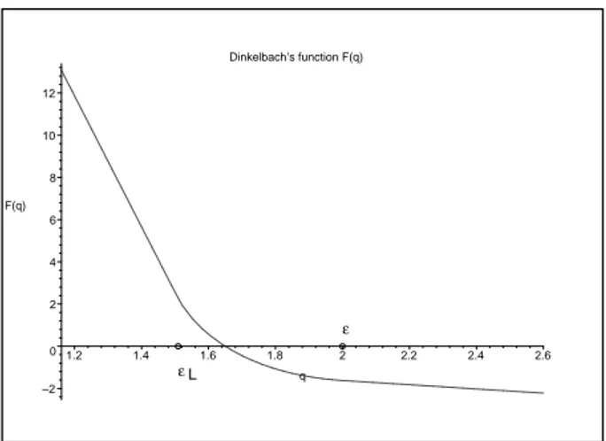
Dinkelbach’s function F(q) L ε ε –2 0 2 4 6 8 10 12 F(q) 1.2 1.4 1.6 1.8 2 2.2 2.4 2.6 q
Figure 1: Graph of Dinkelbach’s function.
In fact, the optimal value q∗ is implicitly defined by the following equation
F (q∗) = 0 .
When δ 6= k function F is differentiable and decreasing, therefore ∂F/∂q < 0 and it is possible to apply the implicit function theorem to obtain the sign of the derivative of q∗ with respect to the parameters. It is thus possible to prove that:
∂q∗ ∂b > 0 ; ∂q∗ ∂δ < 0 ; ∂q∗ ∂A0 > 0 ; ∂q∗ ∂C0 < 0 ; ∂q∗ ∂a ≥ 0 ; ∂q∗ ∂k > 0 ; ∂q∗ ∂² ≥ 0 . 4.2 A numerical example
Consider the case a = 30, k = 3, b = 0.10, T = 1, δ = 4, ² = 2, A0 = 0.1, C0 = 1. Since δ > k
we have case (b) of Propositions 4 and 5, the optimal control will be 0 − a. In Figure 1 we plot function F (q). The optimum value is obtained when F4(q) = 0, a simple numerical computation
allows to find q∗' 1.64960. From (11) we obtain the optimal switch time τ∗ ' 0.69834.
5
Conclusions
In this paper we consider an advertising efficiency maximization problem. The problem turns out to be a linear fractional optimal control problem; to solve it we propose to use the Dinkelbach approach and the particular structure of the functional allows to obtain an (almost) explicit solution of the problem and, in particular, to determine how the structure of the optimal advertising policies changes depending on goodwill’s decay.
The same methodology could be applied to a more general class of fractional functionals, this will be addressed in the next future research.
Moreover, the same efficiency index considered in the objective functional of the advertising problem could be used to compare different advertisers (or different media) in a Data Envelopment Analysis (DEA) framework. This could therefore lead to a dynamic approach to DEA, which will be an other stimulating topic for future research.
6
Appendix
In this appendix we give the proofs of propositions 1-5.
6.1 Proof of Proposition 1
We prove that the Proposition holds for any value of q and therefore also for the optimal value
q∗.
Given problem Pq consider its Hamiltonian function
Hq= kA(t) − qa(t) + p(t)[−δA(t) + ²a(t)] = [k − p(t)δ]A(t) + [p(t)² − q]a(t),
where, due to Pontryagin Maximum Principle, function p(t) is such that ( ˙p(t) = δp(t) − k; p(T ) = 1; i.e. p(t) = µ 1 −k δ ¶ eδ(t−T )+k δ .
Therefore, the switching function is
Gq(t) = p(t)² − q = ²(δ − k)
δ e
δ(t−T )+²k
δ − q . (22)
(a) Let q 6= k²/δ. If δ = k then function (22) is constant and non-zero: positive if ² > q and negative if ² < q; while if δ 6= k then function (22) is not constant and has at most one zero. So if q 6= k²/δ then function (22) has at most one zero. Therefore there exists a unique optimal control of problem Pq and this optimal control is bang-bang with at most one switch.
(b) Let q = k²/δ and δ > k. Then function (22) is
Gq(t) =
²(δ − k)
δ e
δ(t−T ) (23)
and is positive ∀ t ∈ [0, T ]. Therefore the optimal control of Pq is a(t) = a ∀t ∈ [0, T ].
(c) Let q = k²/δ and δ < k. Then function (22) has form (23) and is negative ∀ t ∈ [0, T ]. Therefore the optimal control of Pq is a(t) = 0 ∀t ∈ [0, T ].
(d) Let q = k²/δ and δ = k. Then function (22) is identically zero. Therefore in this case it is not possible to apply the Pontryagin Maximum Principle. But, fortunately, the problem Pq can
Lemma 1 Let q = k²/δ and δ = k. Then F (q) = A0+ kbT − ²C0.
Proof of Lemma 1. Using the motion equation of problem Pqwe can rewrite its objective function
this way (remark that now q = ²)
F (q) = à A(T ) + k Z T 0 (A(t) + b)dt ! − q à C0+ Z T 0 a(t)dt ! = = Z T
0 [kA(t) − qa(t) + kb]dt + A(T ) − qC0 =
= Z T 0 [kA(t) − qa(t)]dt + Z T 0 ˙ A(t)dt + A0+ kbT − qC0= = Z T
0 [kA(t) − qa(t) − δA(t) + ²a(t)]dt + A0+ kbT − qC0=
= A0+ kbT − ²C0 .
¦
Now we can complete the proof of case (d) of the Proposition. Due to Lemma 1, function
F (q) is constant. Therefore in this case any control function a(t) ∈ Adv is optimal for Pq.
¦
6.2 Proof of Proposition 2
Also in this case, we prove that the Proposition holds for any value of q and therefore also for the optimal value q∗.
Due to case (a) of Proposition 1, there exists a unique optimal control of problem Pq and this
optimal control is bang-bang with at most one switch. It means that the optimal control a(t) can be only of form (??) or of form (??).
(a) Let δ > k. Then the switching function (22) increases. Therefore, the optimal control
a(t) has form (??).
(b) Let δ < k. Then the switching function (22) decreases. Therefore, the optimal control
a(t) has form (??).
(c) Let δ = k and q < ². Then the switching function (22) is constant and positive. Therefore, the optimal control of problem F P is a(t) = a ∀ t ∈ [0, T ].
(d) Let δ = k and q > ². Then the switching function (22) is constant and negative. Therefore, the optimal control of problem F P is a(t) = 0 ∀ t ∈ [0, T ].
¦
6.3 Proof of Proposition 3
Let be q∗ such that F (q∗) = 0.
If q∗ = k²/δ and δ = k then any control function a(t) ∈ Adv is optimal, see case (d) of
Proposition 1; moreover F (q∗) = A
0+ bkT − ²C0, see Lemma 1 in the proof of Proposition 1.
Therefore, if A0+ bkT 6= ²C0 then either q∗6= k²/δ or δ 6= k; in the first case, i.e. q∗ 6= k²/δ,
the optimal control of Problem F P is bang-bang due to the case (a) Proposition 1.
If instead q∗ = k²/δ and δ 6= k then the optimal control is either a∗(t) = a ∀ t ∈ [0, T ] or
a∗(t) = 0 ∀ t ∈ [0, T ] (see cases (b) and (c) of Proposition 1), i.e. the control is again bang-bang.
¦
6.4 Proof of Proposition 4
Consider again function (22), i.e. the switching function of problem Pq :
Gq(t) = ²(δ − k) δ e δ(t−T )+ ²k δ − q . One has Gq(t) = 0 ⇔ t = T + 1δ ln²(k − δ)k² − δq .
In particular, it means that Gq(t) can be equal to zero only if (k² − δq)(k − δ) > 0. Moreover,
we can understand when this (unique!) zero τ (see (11)) lies in interval (0, T ). Indeed, 0 < τ < T ⇔ e−δt< k² − δq
²(k − δ) < 1. (24)
If δ > k and k² < δq then (24) gives us (recall that L is defined in (12)) 0 < τ < T ⇔ ²L < q < ²,
while if δ < k and k² < δq then (24) gives
0 < τ < T ⇔ ² < q < ²L.
Finally, if δ > k then k² < δ²L due to (13), while if δ < k then k² > δ²L due to (14). Summarizing the above considerations, we obtain the following properties. 1) Let δ > k. Then function Gq(t) is strictly increasing. Moreover
if q < ²L then Gq(t) > 0 ∀ t ∈ (0, T ); if q ∈ (²L, ²) then Gq(t) ( < 0, if t ∈ (0, τ ); > 0, if t ∈ (τ, T ); if q > ² then Gq(t) < 0 ∀ t ∈ (0, T ).
Therefore case (a) of the Proposition is proved.
2) Let δ < k. Then function Gq(t) is strictly decreasing. Moreover
if q < ² then Gq(t) > 0 ∀ t ∈ (0, T ); if q ∈ (², ²L) then Gq(t) ( > 0, if t ∈ (0, τ ); < 0, if t ∈ (τ, T ); if q > ²L then Gq(t) < 0 ∀ t ∈ (0, T ).
Therefore, case (b) of the Proposition is proved.
3) Let δ = k. Then Gq(t) ≡ ² − q, i.e. function Gq(t) is constant: positive if ² > q and negative if ² < q. Moreover, if q = ² then, due to Lemma 1 (see proof of Proposition 1), function
F (q) is constant, so any control function a(t) ∈ Adv is optimal for Problem Pq. Therefore, case
(c) of the Proposition is proved. ¦
6.5 Proof of Proposition 5
(a) Let δ > k. Then optimal control a(t) of Problem Pq is as in case (a) of Proposition 4. Let
us substitute a(t) in the motion equation and solve it. This way we receive the state variable (goodwill) A(t). If q ≤ ²L then A(t) = µ A0−²a δ ¶ e−δt+²a δ , (25) if q ∈ (²L, ²) then A(t) = A0e−δt, if t ∈ (0, τ ); µ A0−²aδ eδτ ¶ e−δt+²a δ , if t ∈ (τ, T ); (26) if q ≥ ² then A(t) = A0e−δt . (27)
Substituting (25), (26) and (27) in F (q) we receive, respectively, (18), (19) and (20).
(b) Let δ < k. Then optimal control a(t) of Problem Pq is as in case (b) of Proposition 4.
Analogously case (a), we can receive that if q ≤ ² then A(t) is (25); if q ∈ (², ²L) then
A(t) = µ A0− ²a δ ¶ e−δt+²a δ , if t ∈ (0, τ ); · A0−²aδ ³ 1 − e−δτ´¸e−δt, if t ∈ (τ, T ); (28)
while if q ≥ ²L then A(t) is (27). Substituting (25), (28) and (27) in F (q) we receive, respectively, (18), (21) and (20).
(c) Let δ = k. Then optimal control a(t) of Problem Pq is as in case (c) of Proposition 4. Therefore, if q < ² then A(t) is (25); while if q > ² then A(t) is (27). Substituting (25), and (27) in F (q) we receive, respectively, (18) and (20). To finish the proof, it is sufficient to remark that
References
[1] Bhatt S.K., An existence theorem for a fractional control problem Journal of Optimization
Theory and Applications 11 (1973) 379–385.
[2] Bykadorov I., Ellero A. and Moretti E., Minimization of communication expenditure for seasonal products RAIRO Operations Research 36 (2002) 109–127.
[3] Dinkelbach W., On nonlinear fractional programming Management Science 13 (1967) 492– 498.
[4] Favaretto D., Viscolani B., Optimal purchase and advertising for a product with immediate sale start. Top 4 (1996) 301–318.
[5] Feichtinger G., Hartl R. F. and Sethi S. P., Dynamic optimal control models in advertising: recent developments. Management Science 40 (1994) 195–226.
[6] Lilien G.L., Kotler P. and Moorthy K.S., Marketing models.Prentice Hall Int., Englewood Cliffs (1992).
[7] Little J. D. C., Aggregate advertising models: the state of the art. Operations Research 27, 4 (1979) 629–667.
[8] Nerlove M. and Arrow K. J., Optimal advertising policy under dynamic conditions.
Economica 29 (1962) 129–142.
[9] L. S. Pontryagin, V. G. Boltyanskii, R. V. Gamkrelidze and E. F. Mishchenko, The
mathematical theory of optimal processes. Pergamon Press, London et al. (1964).
[10] Seierstad A. and Sydsaeter K., Optimal Control Theory with Economic Applications. North– Holland, Amsterdam (1987).
[11] Sethi S.P., Dynamic optimal control models in advertising: a survey SIAM review 19, 4 (1977).
[12] Sethi S.P., Optimal advertising for the Nerlove-Arrow model under a budget constraint
Operational Research Quarterly 28, 3 (1977) 683–693.
[13] Stancu-Minasian I.M., Fractional programming theory, methods and applications. Kluwer Academic Publishers (1997).
[14] Teng J.T. and Thompson G.L., Optimal strategies for general price-advertising models, in Feichtinger G. (ed.) Optimal Control Theory and Economic Analysis North-Holland (1985), 183-195.
[15] Vidale M. L. and Wolfe H. B., An operations research study for sales response to advertising.
Operations Research 5 (1957) 370–381.