A Class of Preconditioners for Large Indefinite Linear Systems, as by-product of Krylov subspace Methods: Part II

G. Fasano and M. Roma

A class of preconditioners for large

indefinite linear systems, as

by-product of Krylov subspace

methods: Part II

Working Paper n. 5/2011

June 2011

This Working Paper is published ! under the auspices of the Department of

Management at Università Ca’ Foscari Venezia. Opinions expressed herein are those

of the authors and not those of the Department or the University. The Working Paper

series is designed to divulge preliminary or incomplete work, circulated to favour

discussion and comments. Citation of this paper should consider its provisional

A Class of Preconditioners for Large Indefinite Linear

Systems, as by-product of Krylov subspace

Methods: Part II

Giovanni Fasano Massimo Roma

<fasano@unive.it> <roma@dis.uniroma1.it>

Dept. of Management Dip. di Inform. e Sistem. “A. Ruberti” Universit`a Ca’Foscari Venezia SAPIENZA, Universit`a di Roma The Italian Ship Model Basin - INSEAN, CNR

(June 2011)

Abstract. In this paper we consider the parameter dependent class of preconditioners

𝑀_ℎ♯(𝑎, 𝛿, 𝐷) defined in the companion paper [6]. The latter was constructed by using in-formation from a Krylov subspace method, adopted to solve the large symmetric linear system 𝐴𝑥 = 𝑏. We first estimate the condition number of the preconditioned matrix 𝑀_ℎ♯(𝑎, 𝛿, 𝐷)𝐴. Then our preconditioners, which are independent of the choice of the Krylov subspace method adopted, proved to be effective also when solving sequences of slowly changing linear systems, in unconstrained optimization and linear algebra frameworks. A numerical experience is provided to give evidence of the performance of 𝑀_ℎ♯(𝑎, 𝛿, 𝐷).

Keywords: Preconditioners, large indefinite linear systems, large scale nonconvex

opti-mization, Krylov subspace methods.

JEL Classification Numbers: C44, C61.

Correspondence to:

Giovanni Fasano Dept. of Management, Universit`a Ca’ Foscari Venezia

San Giobbe, Cannaregio 873 30121 Venezia, Italy

Phone: [+39] 041-234-6922

Fax: [+39] 041-234-7444

E-mail: fasano@unive.it

∗ _{G.Fasano wishes to thank the Italian Ship Model Basin, CNR - INSEAN institute, for the indirect}

1

Introduction

This paper is focused on both theoretical and computational results, for the parameter dependent class of preconditioners 𝑀_ℎ♯(𝑎, 𝛿, 𝐷), addressed in the companion paper [6]. The latter proposal is specifically suited for large scale problems, and our preconditioners are built using information collected by any Krylov subspace method, when solving the sym-metric linear system 𝐴𝑥 = 𝑏, 𝐴 ∈ IR𝑛×𝑛 indefinite.

There is plenty of real applications and/or theoretical frameworks where the solution of large symmetric linear systems is amenable, including several contexts from nonlinear optimization. Examples of the latter contexts range from truncated Newton methods to KKT systems and interior point methods, not to mention the growing interest for PDE constrained optimization.

The class of preconditioners we propose is computationally cheap (in terms of the num-ber of flops), and the construction of its memnum-bers depends on the structural properties of matrix 𝐴. In particular, when 𝐴 is positive definite, the Krylov subspace method adopted to solve the linear system provides, as by product, a factorization of a tridiagonal matrix, used to define our preconditioners. On the other hand, in case 𝐴 is indefinite, the computation of the eigenpairs of a very small symmetric matrix (say at most 20 × 20) is performed, in order to construct the preconditioners. We remark that our parameter dependent precon-ditioners can be addressed by using a general Krylov subspace method. Moreover, we prove theoretical properties for the preconditioned matrix and we provide results which indicate how to possibly select the preconditioners parameters.

In this paper we experienced our preconditioners in the solution of linear systems from numerical analysis and in nonlinear optimization frameworks. In this regard, we prelimi-narily tested our proposal on significant linear systems from the literature, both including small/medium scale difficult linear systems and large systems. Then, we focused on Newton– Krylov methods (see [13] for a survey), and since our proposal may be extended to indefinite linear systems, we considered both convex and nonconvex problems.

The paper is organized as follows: in Section 2, we describe some properties of our class of preconditioners, recalling the results of the companion paper [6]. Section 3 is devoted to estimate the condition number of the preconditioned system matrix. In Section 4 we provide an extensive numerical experience using our preconditioners, and a section of conclusions and future work completes the paper.

As regards the notations, for a 𝑛 × 𝑛 real matrix 𝑀 we denote with Λ[𝑀 ] the spectrum of 𝑀 ; 𝐼𝑘 is the identity matrix of order 𝑘. We indicate with 𝜅(𝐶) the condition number of the real matrix 𝐶 ∈ IR𝑛×𝑛. Finally, with 𝐶 ≻ 0 we indicate that the matrix 𝐶 is positive definite, 𝑡𝑟(𝐶) and 𝑑𝑒𝑡(𝐶) are the trace and the determinant of 𝐶, while ∥ ⋅ ∥ denotes the Euclidean norm.

2

Our class of preconditioners

We recall here our class of preconditioners defined in the companion paper [6]. On this purpose, consider the indefinite linear system

𝐴𝑥 = 𝑏, (2.1)

where 𝐴 ∈ IR𝑛×𝑛 is symmetric, 𝑛 is large and 𝑏 ∈ IR𝑛. Suppose any Krylov subspace method is used for the solution of (2.1).

Assumption 2.1 Let us consider any Krylov subspace method to solve the symmetric linear system (2.1). Suppose at step ℎ of the Krylov method, with ℎ ≤ 𝑛 − 1, the matrices 𝑅ℎ ∈ IR𝑛×ℎ, 𝑇ℎ ∈ IRℎ×ℎ and the vector 𝑢ℎ+1∈ IR𝑛 are generated, such that

𝐴𝑅ℎ = 𝑅ℎ𝑇ℎ+ 𝜌ℎ+1𝑢ℎ+1𝑒𝑇ℎ, 𝜌ℎ+1∈ IR, (2.2) 𝑇ℎ = ⎧ ⎨ ⎩ 𝑉ℎ𝐵ℎ𝑉_ℎ𝑇, if 𝑇ℎ is indefinite 𝐿ℎ𝐷ℎ𝐿𝑇ℎ, if 𝑇ℎ is positive definite (2.3) where 𝑅ℎ = (𝑢1⋅ ⋅ ⋅ 𝑢ℎ), 𝑢𝑇𝑖 𝑢𝑗 = 0, ∥𝑢𝑖∥ = 1, 1 ≤ 𝑖 ∕= 𝑗 ≤ ℎ, 𝑢𝑇_ℎ+1𝑢𝑖= 0, ∥𝑢ℎ+1∥ = 1, 1 ≤ 𝑖 ≤ ℎ,

𝑇ℎ is symmetric and nonsingular, with eigenvalues 𝜇1, . . . , 𝜇ℎ not all coincident 𝐵ℎ = 𝑑𝑖𝑎𝑔1≤𝑖≤ℎ{𝜇𝑖}, 𝑉ℎ= (𝑣1⋅ ⋅ ⋅ 𝑣ℎ) ∈ IRℎ×ℎ orthogonal, (𝜇𝑖, 𝑣𝑖) is eigenpair of 𝑇ℎ, 𝐷ℎ ≻ 0 is diagonal, 𝐿ℎ is unit lower bidiagonal.

Then, using the notation (see also [8, 6])

∣𝑇ℎ∣def= ⎧ ⎨ ⎩ 𝑉ℎ∣𝐵ℎ∣𝑉ℎ𝑇, ∣𝐵ℎ∣ = 𝑑𝑖𝑎𝑔1≤𝑖≤ℎ{∣𝜇𝑖∣}, if 𝑇ℎ is indefinite, 𝑇ℎ, if 𝑇ℎ is positive definite,

the matrix ∣𝑇ℎ∣ is positive definite, for any choice of 𝐴 and for any integer ℎ. Now, recalling the matrix 𝑀ℎ, along with our class of preconditioners 𝑀_ℎ♯(𝑎, 𝛿, 𝐷)

𝑀_ℎ♯(𝑎, 𝛿, 𝐷) = 𝐷[𝐼𝑛− (𝑅ℎ ∣ 𝑢ℎ+1) (𝑅ℎ ∣ 𝑢ℎ+1)𝑇 ] 𝐷𝑇 ℎ ≤ 𝑛 − 1, + (𝑅ℎ ∣ 𝐷𝑢ℎ+1) ( 𝛿2∣𝑇ℎ∣ 𝑎𝑒ℎ 𝑎𝑒𝑇 ℎ 1 )−1 (𝑅ℎ ∣ 𝐷𝑢ℎ+1)𝑇 (2.4) 𝑀_𝑛♯(𝑎, 𝛿, 𝐷) = 𝑅𝑛∣𝑇𝑛∣−1𝑅𝑇𝑛, (2.5)

Theorem 2.1 Consider any Krylov subspace method to solve the symmetric linear system (2.1). Suppose that Assumption 2.1 holds and the Krylov method performs ℎ ≤ 𝑛 iterations. Let 𝑎 ∈ IR, 𝛿 ∕= 0, and let the matrix 𝐷 ∈ IR𝑛×𝑛 be such that [𝑅ℎ ∣ 𝐷𝑢ℎ+1 ∣ 𝐷𝑅𝑛,ℎ+1] is nonsingular, where 𝑅𝑛,ℎ+1𝑅𝑇_𝑛,ℎ+1 = 𝐼𝑛 − (𝑅ℎ ∣ 𝑢ℎ+1) (𝑅ℎ ∣ 𝑢ℎ+1)𝑇. Then, we have the following properties:

𝑎) the matrix 𝑀_ℎ♯(𝑎, 𝛿, 𝐷) is symmetric. Furthermore

– when ℎ ≤ 𝑛 − 1, for any 𝑎 ∈ IR − {±𝛿(𝑒𝑇_ℎ∣𝑇ℎ∣−1𝑒ℎ)−1/2}, 𝑀ℎ♯(𝑎, 𝛿, 𝐷) is nonsin-gular;

– when ℎ = 𝑛 the matrix 𝑀_ℎ♯(𝑎, 𝛿, 𝐷) is nonsingular;

𝑏) the matrix 𝑀_ℎ♯(𝑎, 𝛿, 𝐷) coincides with 𝑀_ℎ−1 as long as either 𝐷 = 𝐼𝑛 and 𝛿 = 1, or ℎ = 𝑛;

𝑐) for ∣𝑎∣ < ∣𝛿∣(𝑒𝑇_ℎ∣𝑇ℎ∣−1𝑒ℎ)−1/2 the matrix 𝑀_ℎ♯(𝑎, 𝛿, 𝐷) is positive definite. Moreover, if 𝐷 = 𝐼𝑛 the spectrum Λ[𝑀_ℎ♯(𝑎, 𝛿, 𝐷)] is given by

Λ[𝑀_ℎ♯(𝑎, 𝛿, 𝐷)]= Λ [ ( 𝛿2_∣𝑇 ℎ∣ 𝑎𝑒ℎ 𝑎𝑒𝑇 ℎ 1 )−1] ∪ Λ[𝐼𝑛−(ℎ+1)] ; 𝑑) when ℎ ≤ 𝑛 − 1:

– if 𝐷 is nonsingular then 𝑀_ℎ♯(𝑎, 𝛿, 𝐷)𝐴 has at least (ℎ − 3) singular values equal to +1/𝛿2;

– if 𝐷 is nonsingular and 𝑎 = 0 then the matrix 𝑀_ℎ♯(𝑎, 𝛿, 𝐷)𝐴 has at least (ℎ − 2) singular values equal to +1/𝛿2;

𝑒) when ℎ = 𝑛, then 𝑀𝑛♯(𝑎, 𝛿, 𝐷) = 𝑀𝑛−1, Λ[𝑀𝑛] = Λ[∣𝑇𝑛∣] and Λ[𝑀𝑛−1𝐴] = Λ[𝐴𝑀𝑛−1] ⊆ {−1, +1}, i.e. the 𝑛 eigenvalues of 𝑀_ℎ♯(𝑎, 𝛿, 𝐷)𝐴 are either +1 or −1.

Proof: See the companion paper [6].

3

On the condition number of matrix 𝑀

(𝑎, 𝛿, 𝐷)𝐴

In this section we want to estimate the condition number 𝜅(𝑀_ℎ♯(𝑎, 𝛿, 𝐷)𝐴) of the unsymmet-ric matrix 𝑀_ℎ♯(𝑎, 𝛿, 𝐷)𝐴 (where 𝑀_ℎ♯(𝑎, 𝛿, 𝐷) is computed as in (2.4)-(2.5) and 𝐴 is defined in (2.1)). We immediately have

𝜅(𝑀_ℎ♯(𝑎, 𝛿, 𝐷)𝐴) def= ∥𝑀_ℎ♯(𝑎, 𝛿, 𝐷)𝐴∥2⋅ ∥(𝑀_ℎ♯(𝑎, 𝛿, 𝐷)𝐴)−1∥2

= ∥𝑀_ℎ♯(𝑎, 𝛿, 𝐷)𝐴∥2⋅ ∥𝐴−1(𝑀_ℎ♯(𝑎, 𝛿, 𝐷))−1∥2, (3.1) and we can prove the next technical lemma.

Lemma 3.1 Let 𝐶 ∈ IRℎ×ℎ be a symmetric and positive definite matrix. Let 0 < 𝜔1 ≤ ⋅ ⋅ ⋅ ≤ 𝜔ℎ be the ordered eigenvalues of 𝐶, with 𝜔1, . . . , 𝜔ℎ not all coincident, and let 𝑎 ∈ IR, 𝛿 ∈ IR. Then, given the quantities

𝛼 = −𝛿2(ℎ − 1)𝜔1+ 𝛿2𝑡𝑟(𝐶) + 1, 𝛽 = 𝛿2𝑑𝑒𝑡(𝐶) [ 1 −𝑎 2 𝛿2𝑒 𝑇 ℎ𝐶−1𝑒ℎ ] (𝜔ℎ)ℎ−1 , we have 𝛼2− 4𝛽 > 0 In addition [𝑡𝑟(𝐶) − (ℎ − 1)𝜔1] 𝜔ℎ−1_ℎ 𝑑𝑒𝑡(𝐶) > 1. (3.2)

Proof: By the definition of 𝛼 and 𝛽, and since 𝐶 ≻ 0, the condition 𝛼2_{−4𝛽 ≥ 0 is satisfied} if and only if 𝛿2(𝑒𝑇_ℎ𝐶−1𝑒ℎ)−1 [ 1 −𝛼 2_(𝜔 ℎ)ℎ−1 4𝛿2_{𝑑𝑒𝑡(𝐶)} ] ≤ 𝑎2. (3.3)

Now, observing that 𝜔1, . . . , 𝜔ℎ are not all coincident, 𝛼 > 𝛿2𝜔ℎ+ 1 and for any 𝜔1≥ 0 we have (𝛿2_𝜔 1+ 1)2 ≥ 4𝛿2𝜔1, we obtain 𝛼2(𝜔ℎ)ℎ−1 4𝛿2_{𝑑𝑒𝑡(𝐶)} ≥ 𝛼2 4𝛿2_𝜔 1 > (𝛿 2_𝜔 ℎ+ 1)2 4𝛿2_𝜔 1 ≥ (𝛿 2_𝜔 1+ 1)2 4𝛿2_𝜔 1 ≥ 1, (3.4)

so that (3.3) holds for any choice of 𝑎, which also implies that 𝛼2− 4𝛽 ≥ 0. Also observe that by (3.4) 𝛼2(𝜔ℎ)ℎ−1/[4𝛿2𝑑𝑒𝑡(𝐶)] > 1, so that (3.3) can never be satisfied as an equality, i.e. 𝛼2_{− 4𝛽 ∕= 0 for any value of the parameter 𝑎.}

Finally, note that since 𝑑𝑒𝑡(𝐶) = 𝜔1⋅ ⋅ ⋅ ⋅ ⋅ 𝜔ℎ we have

𝜔_ℎℎ−1> 𝑑𝑒𝑡(𝐶)

𝑡𝑟(𝐶) − (ℎ − 1)𝜔1

, (3.5)

inasmuch as 𝜔1, . . . , 𝜔ℎ are not all coincident and 𝑑𝑒𝑡(𝐶) 𝑡𝑟(𝐶) − (ℎ − 1)𝜔1 ≤ 𝑑𝑒𝑡(𝐶) 𝜔ℎ = ℎ−1 ∏ 𝑖=1 𝜔𝑖 < 𝜔ℎ−1_ℎ . As a consequence, we have the condition

[𝑡𝑟(𝐶) − (ℎ − 1)𝜔1] 𝜔ℎ−1ℎ

In the following result we provide a general estimation of the condition number 𝜅(𝑀_ℎ♯(𝑎, 𝛿, 𝐷)𝐴), which depends on the parameters ‘𝛿’ and ‘𝑎’, and the matrix ‘𝐷’ in (2.4). Note that for the sake of clarity, but with a little abuse of notation, in the sequel we directly indicate with 𝜇1, . . . , 𝜇ℎ the eigenvalues of ∣𝑇ℎ∣ and not the eigenvalues of 𝑇ℎ.

Proposition 3.2 Consider the matrix 𝑀_ℎ♯(𝑎, 𝛿, 𝐷) in (2.4)-(2.5), with ℎ ≤ 𝑛 − 1, where ∣𝑇ℎ∣ satisfies Assumption 2.1. Let 𝜇1 ≤ ⋅ ⋅ ⋅ ≤ 𝜇ℎ be the (ordered) eigenvalues of ∣𝑇ℎ∣, where 𝜇1, . . . , 𝜇ℎ are not all coincident. Then, if

∣𝑎∣ < ∣𝛿∣(𝑒𝑇_ℎ∣𝑇ℎ∣−1𝑒ℎ)−1/2, 𝛿 ∕= 0 (3.7) we have 𝜅(𝑀_ℎ♯(𝑎, 𝛿, 𝐷)𝐴) ≤ 𝜉ℎ⋅ 𝜅(𝑁 )2⋅ 𝜅(𝐴), (3.8) with 𝜉ℎ = max{1,𝛾ℎ+(𝛾ℎ2−4𝜎ℎ)1/2 2 } min{1,𝛾ℎ−(𝛾ℎ2−4𝜎ℎ)1/2 2 } ≥ 1 (3.9) and 𝛾ℎ = −𝛿2(ℎ − 1)𝜇1+ 𝛿2𝑡𝑟(∣𝑇ℎ∣) + 1 𝜎ℎ = 𝛿2_{𝑑𝑒𝑡(∣𝑇} ℎ∣) [ 1 −𝑎_𝛿22𝑒𝑇_ℎ∣𝑇ℎ∣−1𝑒ℎ ] (𝜇ℎ)ℎ−1 . In particular, when 𝐷 = 𝐼𝑛 in (2.4) then 𝜅(𝑀_ℎ♯𝐴) ≤ 𝜉ℎ⋅ 𝜅(𝐴).

Proof: Let 𝜆1 ≤ ⋅ ⋅ ⋅ ≤ 𝜆ℎ+1 be the (ordered) eigenvalues of the matrix (

𝛿2∣𝑇ℎ∣ 𝑎𝑒ℎ

𝑎𝑒𝑇_ℎ 1

)

, (3.10)

which is positive definite as long as condition (3.7) is fulfilled. Observe that by the identity ( 𝛿2_∣𝑇 ℎ∣ 𝑎𝑒ℎ 𝑎𝑒𝑇_ℎ 1 ) = ( 𝐼ℎ 0 𝑎 𝛿2𝑒𝑇_ℎ∣𝑇ℎ∣−1 1 ) ( 𝛿2∣𝑇ℎ∣ 0 0 1 −𝑎_𝛿22𝑒𝑇_ℎ∣𝑇ℎ∣−1𝑒ℎ ) ( 𝐼ℎ _𝛿𝑎2∣𝑇ℎ∣−1𝑒ℎ 0 1 ) we have 𝑑𝑒𝑡 ( 𝛿2∣𝑇ℎ∣ 𝑎𝑒ℎ 𝑎𝑒𝑇_ℎ 1 ) = 𝛿2ℎ𝑑𝑒𝑡(∣𝑇ℎ∣) [ 1 −𝑎 2 𝛿2𝑒 𝑇 ℎ∣𝑇ℎ∣−1𝑒ℎ ] (3.11) and 𝛿2∣𝑇ℎ∣ is the ℎ × ℎ upper left diagonal block of matrix (3.10). Therefore, by the Cauchy interlacing properties [4] between the sequences {𝜇𝑗}𝑗=1,...,ℎ and {𝜆𝑖}𝑖=1,...,ℎ+1 we have

𝜆1 ≤ 𝛿2𝜇1 ≤ 𝜆2≤ 𝛿2𝜇2 ≤ ⋅ ⋅ ⋅ ≤ 𝜆ℎ≤ 𝛿2𝜇ℎ ≤ 𝜆ℎ+1. (3.12) By (3.10), (3.11) and (3.12) we can immediately infer the following intermediate results:

1. 𝛿2_𝜇

2. ℎ+1 ∑ 𝑖=1 𝜆𝑖= 𝛿2𝑡𝑟(∣𝑇ℎ∣) + 1 3. ℎ+1 ∏ 𝑖=1 𝜆𝑖 = 𝛿2ℎ𝑑𝑒𝑡(∣𝑇ℎ∣) [ 1 − 𝑎 2 𝛿2𝑒 𝑇 ℎ∣𝑇ℎ∣−1𝑒ℎ ]

From 1. we deduce that

𝛿2(ℎ − 1)𝜇1 ≤ ℎ ∑

𝑖=2

𝜆𝑖 ≤ 𝛿2(ℎ − 1)𝜇ℎ,

so that from 2., 3., (3.12) and recalling that the matrix (3.10) is positive definite, we have max{0, −𝛿2_{(ℎ − 1)𝜇} ℎ+ 𝛿2𝑡𝑟(∣𝑇ℎ∣) + 1 } ≤ 𝜆1+ 𝜆ℎ+1 ≤ −𝛿2(ℎ − 1)𝜇1+ 𝛿2𝑡𝑟(∣𝑇ℎ∣) + 1 𝛿2ℎ𝑑𝑒𝑡(∣𝑇ℎ∣) [ 1 − 𝑎_𝛿22𝑒𝑇_ℎ∣𝑇ℎ∣−1𝑒ℎ ] 𝛿2(ℎ−1)_(𝜇 ℎ)ℎ−1 ≤ 𝜆1⋅ 𝜆ℎ+1 ≤ 𝛿2ℎ𝑑𝑒𝑡(∣𝑇ℎ∣) [ 1 −𝑎_𝛿22𝑒𝑇_ℎ∣𝑇ℎ∣−1𝑒ℎ ] 𝛿2(ℎ−1)_(𝜇 1)ℎ−1 . (3.13) From (3.13) (see also points (𝐴) and (𝐵) in Figure 3.1), in order to compute bounds 𝜆1

λ₁ λh+1 λ₁ + λ_h+1 = − δ2 (h−1)µ₁ + δ2 tr (|T_h|) +1 λ₁ + λ_h+1 = = − δ2 (h−1)µ_h + δ2 tr (|T_h|) +1

.

.

Figure 3.1: Relation between the eigenvalues 𝜆1 and 𝜆ℎ+1of matrix (3.10).

[𝜆ℎ+1] for the smallest [largest] eigenvalue of matrix (3.10), we have to solve the linear system (𝜎ℎ and 𝛾ℎ are defined in the statement of this proposition)

{ ˜

𝜆1+ ˜𝜆ℎ+1= 𝛾ℎ ˜

which yields ˜ 𝜆1= 𝛾ℎ−(𝛾 2 ℎ−4𝜎ℎ)1/2 2 ˜ 𝜆ℎ+1= 𝛾ℎ+(𝛾 2 ℎ−4𝜎ℎ)1/2 2 , (3.14)

provided that 𝛾_ℎ2− 4𝜎ℎ ≥ 0. However, the latter condition directly holds from Lemma 3.1.

Now, observe that from Theorem 2.1, setting 𝑁 = [𝑅ℎ ∣ 𝐷𝑢ℎ+1 ∣ 𝐷𝑅𝑛,ℎ+1] (where 𝑁 is

nonsingular by hypothesis), for ℎ ≤ 𝑛 − 1 the preconditioners 𝑀_ℎ♯(𝑎, 𝛿, 𝐷) may be rewritten as 𝑀_ℎ♯(𝑎, 𝛿, 𝐷) = 𝑁 ⎡ ⎣ ( 𝛿2∣𝑇ℎ∣ 𝑎𝑒ℎ 𝑎𝑒𝑇 ℎ 1 )−1 0 0 𝐼𝑛−(ℎ+1) ⎤ ⎦𝑁𝑇, ℎ ≤ 𝑛 − 1. (3.15) As a consequence, setting 𝑊ℎ= ⎡ ⎣ ( 𝛿2∣𝑇ℎ∣ 𝑎𝑒ℎ 𝑎𝑒𝑇_ℎ 1 ) 0 0 𝐼𝑛−(ℎ+1) ⎤ ⎦,

we have for the smallest [largest] eigenvalue 𝜆𝑚 [𝜆𝑀] of matrices 𝑊ℎ and 𝑊_ℎ−1 the expres-sions ⎧ ⎨ ⎩ 𝜆𝑚(𝑊ℎ) = min {1, 𝜆1} 𝜆𝑀(𝑊ℎ) = max {1, 𝜆ℎ+1} ⎧  ⎨  ⎩ 𝜆𝑚(𝑊_ℎ−1) = _max{1,𝜆1 _ℎ+1} 𝜆𝑀(𝑊_ℎ−1) = _min{1,𝜆1 _1}.

Thus, if 𝜆𝑚(𝐴) [𝜆𝑚(𝐴−1)] and 𝜆𝑀(𝐴) [𝜆𝑀(𝐴−1)] are the smallest [largest] eigenvalue of matrix 𝐴 [𝐴−1] respectively, from (3.15) we have

∥𝑀_ℎ♯(𝑎, 𝛿, 𝐷)𝐴∥ ≤ 𝜆𝑀(𝐴) ⋅ ∥𝑁 ∥2⋅ 𝜆𝑀(𝑊ℎ−1) ≤ 𝜆𝑀(𝐴) ⋅ ∥𝑁 ∥2⋅ 1 min {1, 𝜆1} and ∥(𝑀_ℎ♯(𝑎, 𝛿, 𝐷)𝐴)−1∥ = ∥𝐴−1(𝑀_ℎ♯(𝑎, 𝛿, 𝐷))−1∥ ≤ 𝜆𝑀(𝐴−1) ⋅ ∥𝑁−1∥2⋅ 𝜆𝑀(𝑊ℎ) ≤ 1 𝜆𝑚(𝐴) ⋅ ∥𝑁−1∥2⋅ max {1, 𝜆ℎ+1} , so that from (3.14) 𝜅(𝑀_ℎ♯(𝑎, 𝛿, 𝐷)𝐴) = ∥𝑀_ℎ♯(𝑎, 𝛿, 𝐷)𝐴∥ ⋅ ∥(𝑀_ℎ♯(𝑎, 𝛿, 𝐷)𝐴)−1∥ ≤ max{1, ˜𝜆ℎ+1 } min{1, ˜𝜆1 } 𝜅(𝑁 ) 2_𝜅(𝐴),

In order to better specify the bound (3.8) we can now prove the next lemma.

Lemma 3.3 Let us consider the hypotheses of Proposition 3.2 and the quantity 𝜉ℎ defined in (3.9). Then, for any choice of ‘𝛿’ and ‘𝑎’ satisfying (3.7) we have

𝜉ℎ=

𝛾ℎ+ (𝛾_ℎ2− 4𝜎ℎ)1/2 𝛾ℎ− (𝛾ℎ2− 4𝜎ℎ)1/2

. (3.16)

Proof: The proof consists to analyze the following three cases: 1. 𝛾ℎ < 2 (i.e. 𝛿2 < 1/[𝑡𝑟(∣𝑇ℎ∣) − (ℎ − 1)𝜇1])

2. 𝛾ℎ = 2 (i.e. 𝛿2 = 1/[𝑡𝑟(∣𝑇ℎ∣) − (ℎ − 1)𝜇1]) 3. 𝛾ℎ > 2 (i.e. 𝛿2 > 1/[𝑡𝑟(∣𝑇ℎ∣) − (ℎ − 1)𝜇1]) In case 1. is satisfied, observe that the inequality

𝛾ℎ+ (𝛾ℎ2− 4𝜎ℎ)1/2

2 < 1

cannot hold, since (consider that 𝛾ℎ− 2 < 0 and see Lemma 3.1) it requires that 𝛾ℎ < 1 + 𝜎ℎ iff 𝑎2 < [ 1 −(𝛾ℎ− 1)𝜇 ℎ−1 ℎ 𝛿2_{𝑑𝑒𝑡(∣𝑇} ℎ∣) ] 𝛿2 𝑒𝑇 ℎ∣𝑇ℎ∣−1𝑒ℎ which can hold only if

(𝛾ℎ− 1)𝜇ℎ−1ℎ 𝛿2_{𝑑𝑒𝑡(∣𝑇} ℎ∣) ≤ 1 or equivalently 𝛿2 ≥ (𝛾ℎ− 1)𝜇 ℎ−1 ℎ 𝑑𝑒𝑡(∣𝑇ℎ∣) .

However, the last inequality cannot hold because it is equivalent to 1 ≥ [𝑡𝑟(∣𝑇ℎ∣) − (ℎ − 1)𝜇1]𝜇

ℎ−1 ℎ 𝑑𝑒𝑡(∣𝑇ℎ∣)

,

which cannot be satisfied from Lemma 3.1. Moreover, in case 1., also 𝛾ℎ− (𝛾ℎ2− 4𝜎ℎ)1/2

2 > 1

cannot hold, since 𝛾ℎ− 2 < 0. Therefore, when 𝛾ℎ < 2 relation (3.16) holds.

The case 2. is pretty similar to the case 1., so that again (3.16) follows almost immedi-ately.

In case 3., the inequality

𝛾ℎ+ (𝛾ℎ2− 4𝜎ℎ)1/2

cannot hold since it is equivalent to (𝛾2

ℎ − 4𝜎ℎ)1/2 < 2 − 𝛾ℎ < 0. Moreover, from Lemma 3.1 and considering that 𝛾ℎ− 2 > 0, the condition

𝛾ℎ− (𝛾ℎ2− 4𝜎ℎ)1/2 2 > 1 can be satisfied if 𝛾ℎ< 1 + 𝜎ℎ iff 𝑎2 < [ 1 − (𝛾ℎ− 1)𝜇 ℎ−1 ℎ 𝛿2_{𝑑𝑒𝑡(∣𝑇} ℎ∣) ] 𝛿2 𝑒𝑇 ℎ∣𝑇ℎ∣−1𝑒ℎ , which holds only if

(𝛾ℎ− 1)𝜇ℎ−1ℎ 𝛿2_{𝑑𝑒𝑡(∣𝑇} ℎ∣) ≤ 1 or equivalently 𝛿2 ≥ (𝛾ℎ− 1)𝜇 ℎ−1 ℎ 𝑑𝑒𝑡(∣𝑇ℎ∣) .

However, since 𝛾ℎ− 1 = 𝑡𝑟(∣𝑇ℎ∣) − (ℎ − 1)𝜇1, the last inequality is again equivalent to 1 ≥ [𝑡𝑟(∣𝑇ℎ∣) − (ℎ − 1)𝜇1]𝜇

ℎ−1 ℎ 𝑑𝑒𝑡(∣𝑇ℎ∣)

which cannot hold from Lemma 3.1. Thus relation (3.16) holds.

Lemma 3.4 Consider the matrix 𝑀_ℎ♯(𝑎, 𝛿, 𝐷) in (2.4)-(2.5), with ℎ ≤ 𝑛. Let 𝜇1 ≤ ⋅ ⋅ ⋅ ≤ 𝜇ℎ be the (ordered) eigenvalues of ∣𝑇ℎ∣, with 𝜇1, ⋅ ⋅ ⋅ , 𝜇ℎnot all coincident, and let the parameters ‘𝑎’ and ‘𝛿’ satisfy condition (3.7). Then, for any choice of the matrix 𝐷 in (2.4)

∙ the coefficient 𝜉ℎ in (3.9) increases when ∣𝑎∣ → 𝜌, with 𝜌 = ∣𝛿∣(𝑒𝑇ℎ∣𝑇ℎ∣−1𝑒ℎ)−1/2, and lim

∣𝑎∣→𝜌𝜉ℎ = +∞

∙ the coefficient 𝜉ℎ in (3.9) attains its minimum when 𝑎 = 0, and for 𝑎 = 0 we have for the coefficient 𝜉ℎ in (3.9) the expression

𝜉ℎ = 𝛾ℎ+ ( 𝛾2 ℎ− 4 𝛿2 𝑑𝑒𝑡(∣𝑇ℎ∣) (𝜇ℎ)ℎ−1 )1/2 𝛾ℎ− ( 𝛾_ℎ2− 4𝛿2𝑑𝑒𝑡(∣𝑇ℎ∣) (𝜇ℎ)ℎ−1 )1/2. (3.17)

Proof: Observe that when ∣𝑎∣ → 𝜌 then in the expression (3.9) of 𝜉ℎ we have 𝜎ℎ → 0,

along with 𝛾ℎ − (𝛾ℎ2 − 4𝜎ℎ)1/2 → 0 and 𝛾ℎ + (𝛾ℎ2 − 4𝜎ℎ)1/2 → 2𝛾ℎ, with 𝛾ℎ > 1. Thus, since from Lemma 3.1 𝛾ℎ− 4𝜎ℎ ≥ 0, Lemma 3.3 ensures that 𝜉ℎ satisfies (3.16), so that

𝜉ℎ increases as ∣𝑎∣ → 𝜌, with lim∣𝑎∣→𝜌𝜉¯ℎ = +∞. Moreover, from (3.16) and since 𝜉ℎ is a continuous function of the parameter ‘𝑎’ (see (3.7)), we have

∂𝜉ℎ ∂𝑎 = ∂𝜉ℎ ∂𝜎ℎ ⋅∂𝜎ℎ ∂𝑎 = −2𝛾ℎ [𝛾ℎ− (𝛾_ℎ2+ 4𝜎ℎ)1/2]2(𝛾_ℎ2− 4𝜎ℎ)1/2 ⋅−2𝑎 ⋅ 𝑑𝑒𝑡(∣𝑇ℎ∣)𝑒 𝑇 ℎ∣𝑇ℎ∣−1𝑒ℎ (𝜇ℎ)ℎ−1 , so that for ∣𝑎∣ < 𝜌 we have 𝑠𝑔𝑛{∂𝜉ℎ/∂𝑎} = 𝑠𝑔𝑛{𝑎}, which implies that 𝜉ℎ attains its minimum for 𝑎 = 0.

Finally, by Lemma 3.1 𝛾2

ℎ− 4𝜎ℎ≥ 0 for any choice of 𝑎 satisfying (3.7), and when 𝑎 = 0 it is 𝜎ℎ = 𝛿2𝑑𝑒𝑡(∣𝑇ℎ∣)/(𝜇ℎ)ℎ−1. Thus, from Lemma 3.3 the value of 𝜉ℎ when 𝑎 = 0 is given by 𝜉ℎ = 𝛾ℎ+ ( 𝛾2_ℎ− 4𝛿2𝑑𝑒𝑡(∣𝑇ℎ∣) (𝜇ℎ)ℎ−1 )1/2 𝛾ℎ− ( 𝛾2 ℎ− 4 𝛿2_{𝑑𝑒𝑡(∣𝑇} ℎ∣) (𝜇ℎ)ℎ−1 )1/2, so that (3.17) holds.

Remark 3.1 By (3.17) we observe that as expected, the parameter ‘𝛿’ both affects the

distribution of the singular values of 𝑀_ℎ♯(𝑎, 𝛿, 𝐷)𝐴 (see item 𝑑) of Theorem 2.1), and also its condition number 𝜅(𝑀_ℎ♯(𝑎, 𝛿, 𝐷)𝐴), when computed according with (3.1).

4

Preliminary numerical results

In order to preliminarily test our proposal on a general framework, where no information is known about the sparsity pattern of the matrix 𝐴, we used our parameter dependent class of preconditioners 𝑀_ℎ♯(𝑎, 𝛿, 𝐷), setting 𝛿 = 1 and 𝐷 = 𝐼𝑛.

In our numerical experience we obtain even better results w.r.t. the theory. Indeed, all the results assessed in Theorem 2.1 for the singular values of the (possibly) unsymmetric matrix 𝑀_ℎ♯(𝑎, 𝛿, 𝐷)𝐴, seem to hold in practice also for the eigenvalues of 𝑀_ℎ♯(𝑎, 𝛿, 𝐷)𝐴 (we recall that since 𝑀_ℎ♯(𝑎, 𝛿, 𝐷) ≻ 0 then Λ[𝑀_ℎ♯(𝑎, 𝛿, 𝐷)𝐴] ≡ Λ[𝑀_ℎ♯(𝑎, 𝛿, 𝐷)1/2𝐴𝑀_ℎ♯(𝑎, 𝛿, 𝐷)1/2]), so that 𝑀_ℎ♯(𝑎, 𝛿, 𝐷)𝐴 has only real eigenvalues. In order to test the class of preconditioners (2.4)-(2.5), we used 4 different sets of test problems.

First, we considered a set of symmetric linear systems as in (2.1), where the number of unknowns 𝑛 is set as 𝑛 = 1000, and the matrix 𝐴 has also a moderate condition number. We simply wanted to experience how our class of preconditioners modifies the condition number of 𝐴. In particular (see also [7]), a possible choice for the latter class of matrices is given by

𝐴 = {𝑎𝑖,𝑗}, 𝑎𝑖𝑗 ∈ 𝑈 [−10, 10], 𝑖, 𝑗 = 1, . . . , 𝑛, (4.1)

where 𝑎𝑖,𝑗 = 𝑎𝑗,𝑖 are random entries in the uniform distribution 𝑈 [−10, 10], between −10 and +10. Then, also the vector 𝑏 in (2.1) is computed randomly with entries in the set 𝑈 [−10, 10]. We computed the preconditioners (2.4)-(2.5) by using the Conjugate Gradient

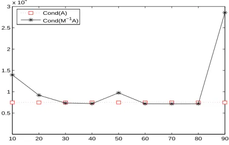
10 20 30 40 50 60 70 80 90 0.5 1 1.5 2 2.5 3x 10 4 Cond(A) Cond(M−1A)

Figure 4.1: The condition number of matrix 𝐴 (𝐶𝑜𝑛𝑑(𝐴)) along with the condition number of matrix 𝑀_ℎ♯(0, 1, 𝐼)𝐴 (𝐶𝑜𝑛𝑑(𝑀−1𝐴)), when ℎ ∈ {10, 20, 30, 40, 50, 60, 70, 80, 90}, and 𝐴 is randomly chosen with entries in the uniform distribution 𝑈 [−10, 10].

(CG) method [16], which is one of the most popular Krylov subspace methods to solve (2.1) [9]. We remark that the CG is often used also in case the matrix 𝐴 is indefinite, though it can prematurely stop. As an alternative choice, in order to satisfy Assumption 2.1 with 𝐴 indefinite, we can use the Lanczos process [11], MINRES methods [15] or Planar-CG methods [5]. In (2.4) we set the parameter ℎ in the range

ℎ ∈ { 20 , 30 , 40 , 50 , 60 , 70 , 80 , 90 },

and we preliminarily chose 𝑎 = 0 (though other choices of the parameter ‘𝑎’ yield similar results), which satisfied items 𝑎) and 𝑐) of Theorem 2.1. We plotted in Figure 4.1 the condition number 𝜅(𝐴) of 𝐴 (𝐶𝑜𝑛𝑑(𝐴)), along with the condition number 𝜅(𝑀_ℎ♯(0, 1, 𝐼)𝐴) of 𝑀_ℎ♯(0, 1, 𝐼)𝐴 (𝐶𝑜𝑛𝑑(𝑀−1_{𝐴)): in both cases the condition number 𝜅 is calculated by} preliminarily computing the eigenvalues 𝜆1, . . . , 𝜆𝑛 (using Matlab [1] routine eigs()) of 𝐴 and 𝑀_ℎ♯(0, 1, 𝐼)𝐴 respectively, then obtaining the ratio

𝜅 = max𝑖 ∣𝜆𝑖∣ min𝑖 ∣𝜆𝑖∣ .

Evidently, numerical results confirm that the order of the condition number of 𝐴 is pretty similar to that of the condition number of 𝑀_ℎ♯(0, 1, 𝐼)𝐴. This indicates that if the precon-ditioners (2.4) are used as a tool to solve (2.1), then most preconditioned iterative methods which are sensible to the condition number (e.g. the Krylov subspace methods), on average are not expected to perform worse with respect to the unpreconditioned case. However, it is important to remark that the spectrum Λ[𝑀_ℎ♯(0, 1, 𝐼)𝐴] tends to be shifted with respect

0 200 400 600 800 1000 −300 −200 −100 0 100 200 300 Unprecond Precond (h5) 450 500 550 −25 −20 −15 −10 −5 0 5 10 15 20 25 Unprecond Precond (h5) 0 200 400 600 800 1000 −300 −200 −100 0 100 200 300 Unprecond Precond (h6) 450 500 550 −25 −20 −15 −10 −5 0 5 10 15 20 25 Unprecond Precond (h6)

Figure 4.2: Comparison between the full/detailed spectra (left/right figures) Λ[𝐴] (Unpre-cond) and Λ[𝑀_ℎ♯(0, 1, 𝐼)𝐴] (Precond), with 𝐴 randomly chosen (eigenvalues are sorted for simplicity); without loss of generality we show the results for the values ℎ = ℎ5 = 20 and ℎ = ℎ6 = 30. The intermediate eigenvalues in the spectrum Λ[𝑀_ℎ♯(0, 1, 𝐼)𝐴], whose absolute value is larger than 1, are in general smaller than the corresponding eigenvalues in Λ[𝐴]. The eigenvalues in Λ[𝑀_ℎ♯(0, 1, 𝐼)𝐴] are more clustered near +1 or −1 than those in Λ[𝐴]. to Λ[𝐴], inasmuch as the eigenvalues in Λ[𝐴] whose absolute value is larger than +1 tend to be scaled in Λ[𝑀_ℎ♯(0, 1, 𝐼)𝐴] (see Figure 4.2). The latter property is an appealing result, since the eigenvalues of 𝑀_ℎ♯(0, 1, 𝐼)𝐴 will be ‘more clustered’. The latter phenomenon has been better investigated by introducing other sets of test problems, described hereafter.

In a second experiment we generated the set of matrices 𝐴 such that

𝐴 = 𝐻𝒟𝐻, (4.2)

where 𝐻 ∈ IR𝑛×𝑛, 𝑛 = 500, is an Householder transformation given by 𝐻 = 𝐼 − 2𝑣𝑣𝑇, with 𝑣 ∈ IR𝑛 a unit vector, randomly chosen. The matrix 𝒟 ∈ IR𝑛×𝑛 is diagonal (so that its non-zero entries are also eigenvalues of 𝐴, while each column of 𝐻 is also an eigenvector of 𝐴). The matrix 𝒟 is such that its perc ⋅ 𝑛 eigenvalues are larger (about one order of magnitude) than the remaining (1 − perc) ⋅ 𝑛 eigenvalues (we set without loss of generality

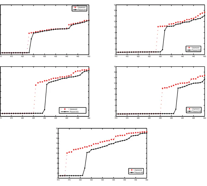
perc= 0.3). Finally, again we computed the preconditioners (2.4)-(2.5) by using the CG, setting the starting point 𝑥0 so that the initial residual 𝑏 − 𝐴𝑥0 was a linear combination (with coefficients −1 and +1 randomly chosen) of all the 𝑛 eigenvectors of 𝐴. We strongly highlight that the latter choice of 𝑥0 is expected to be not favorable when applying the CG, to build our preconditioners. In the latter case the CG method is indeed expected to perform exactly 𝑛 iterations before stopping (see also [14, 16]), so that the matrices (4.2) may be significant to test the effectiveness of our preconditioners, in case of small values of ℎ (broadly speaking, ℎ small implies that the preconditioner contains correspondingly a little information on the inverse matrix 𝐴−1). We compared the spectra Λ[𝐴] and Λ[𝑀_ℎ♯(𝑎, 1, 𝐼)𝐴], in order to verify again how the preconditioners (2.4) are able to cluster the eigenvalues of 𝐴. Following exactly the choice in [12], in order to test our proposal also on a different range of values for the parameter ℎ, we set

ℎ ∈ { 4 , 8 , 12 , 16 , 20 }.

The results are given in Figure 4.3 (full comparisons) which includes all the 500 eigenvalues, and Figure 4.4 (details) which includes only the eigenvalues from the 410-th to the 450-th. Observe that our preconditioners are able to shift the largest absolute eigenvalues of 𝐴 towards −1 or +1, so that the clustering of the eigenvalues is enhanced when the param-eter ℎ increases. For any value of ℎ the matrix 𝐴 is (randomly) recomputed from scratch, according with relation (4.2). This explains while in the five plots of Figures 4.3-4.4 the spectrum of 𝐴 changes. Again, a behavior very similar to Figures 4.3-4.4 is obtained also using different values for the parameter ‘𝑎’.

We used another small set of test problems, obtained by considering a couple of linear systems as (2.1), described in [12, 3] and therein references, which come up from finite ele-ment problems. We addressed the latter linear systems as 𝐴0𝑥 = 𝑏0 (from one-dimensional model, consisting of a line of two-node elements with support conditions at both ends, and a linearly varying body force) and 𝐴1𝑥 = 𝑏1 (where 𝐴1 is the stiffness matrix from a two-dimensional finite element model of a cantilever beam) respectively [12]. The spectral prop-erties of both the matrices 𝐴0 and 𝐴1 are extensively described in [12]. In particular 𝐴0 ∈ IR50×50 is positive definite with condition number 𝜅(𝐴0) = 0.20𝐸 + 10 and with a suitable pattern of clustering of the eigenvalues; similarly, 𝐴1 ∈ IR170×170 is also positive definite, with condition number 𝜅(𝐴1) = 0.13𝐸 + 9 and a different pattern of eigenvalues clustering. In addition, we have

𝑏0= ⎛ ⎜ ⎜ ⎜ ⎜ ⎜ ⎜ ⎜ ⎝ 0 200/49 300/49 .. . 4900/49 0 ⎞ ⎟ ⎟ ⎟ ⎟ ⎟ ⎟ ⎟ ⎠ , 𝑏1 = 0, but 𝑏1(34) = 𝑏1(68) = 𝑏1(102) = 𝑏1(136) = 𝑏1(170) = −8000,

0 50 100 150 200 250 300 350 400 450 500 −30 −20 −10 0 10 20 30 Unprecond Precond (h1) 0 50 100 150 200 250 300 350 400 450 500 −60 −50 −40 −30 −20 −10 0 10 20 30 Unprecond Precond (h2) 0 50 100 150 200 250 300 350 400 450 500 −40 −20 0 20 40 60 80 Unprecond Precond (h3) 0 50 100 150 200 250 300 350 400 450 500 −30 −20 −10 0 10 20 30 Unprecond Precond (h4) 0 50 100 150 200 250 300 350 400 450 500 −30 −20 −10 0 10 20 30 Unprecond Precond (h5)

Figure 4.3: Comparison between the full spectra Λ[𝐴] (Unprecond) and Λ[𝑀_ℎ♯(0, 1, 𝐼)𝐴] (Precond), with 𝐴 nonsingular and given by (4.2) (eigenvalues are sorted for simplicity); we used different values of ℎ (ℎ1 = 4, ℎ2 = 8, ℎ3 = 12, ℎ4 = 16, ℎ5 = 20), setting 𝑛 = 500. The large eigenvalues in the spectrum Λ[𝑀_ℎ♯(0, 1, 𝐼)𝐴] are in general smaller (in modulus) than the corresponding large eigenvalues in Λ[𝐴]. A ‘flatter’ piecewise-line of the eigenvalues in Λ[𝑀_ℎ♯(0, 1, 𝐼)𝐴] indicates that the eigenvalues tend to cluster around −1 and +1, according with the theory.

410 415 420 425 430 435 440 445 450 0 5 10 15 20 25 Unprecond Precond (h1) 410 415 420 425 430 435 440 445 450 0 2 4 6 8 10 12 14 16 18 Unprecond Precond (h2) 410 415 420 425 430 435 440 445 450 0 2 4 6 8 10 12 14 16 Unprecond Precond (h3) 410 415 420 425 430 435 440 445 450 0 2 4 6 8 10 12 14 16 18 Unprecond Precond (h4) 410 415 420 425 430 435 440 445 450 0 2 4 6 8 10 12 14 16 18 20 Unprecond Precond (h5)

Figure 4.4: Comparison between a detail of the spectra Λ[𝐴] (Unprecond) and

Λ[𝑀_ℎ♯(0, 1, 𝐼)𝐴] (Precond), with 𝐴 nonsingular and given by (4.2) (eigenvalues are sorted for simplicity; we used different values of ℎ (ℎ1 = 4, ℎ2 = 8, ℎ3 = 12, ℎ4 = 16, ℎ5 = 20), setting 𝑛 = 500. The large eigenvalues in the spectrum Λ[𝑀_ℎ♯(0, 1, 𝐼)𝐴] are in general smaller (in modulus) than the corresponding large eigenvalues in Λ[𝐴]. A ‘flatter’ piecewise-line of the eigenvalues in Λ[𝑀_ℎ♯(0, 1, 𝐼)𝐴] indicates that the eigenvalues tend to cluster around −1 and +1, according with the theory.

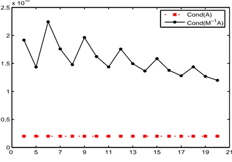
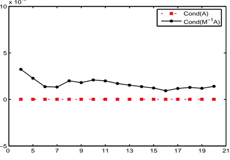
0 5 7 9 11 13 15 17 19 21 0 0.5 1 1.5 2 2.5x 10 10 Cond(A) Cond(M−1A)

Figure 4.5: The condition number of matrix 𝐴0 (𝐶𝑜𝑛𝑑(𝐴)) along with the condition number of matrix 𝑀_ℎ♯(0, 1, 𝐼)𝐴0 (𝐶𝑜𝑛𝑑(𝑀−1𝐴)), when 4 ≤ ℎ ≤ 20. The condition number of 𝐴0 is slightly larger than the condition number of 𝑀_ℎ♯(0, 1, 𝐼)𝐴0, for any value of the parameter ℎ. The starting point of the CG is 𝑥0 = 0.

and the CG is again used to compute the preconditioner 𝑀_ℎ♯(0, 1, 𝐼), adopting both the starting points 𝑥0 = 0 and 𝑥0 = 100, 𝑒 = (1 ⋅ ⋅ ⋅ 1)𝑇, as indicated in [12].

We have computed our class of preconditioners for the linear systems 𝐴0𝑥 = 𝑏0 and

𝐴1𝑥 = 𝑏1, with 𝑎 = 1 and ℎ ∈ {4, 8, 12, 16, 20}. The effect of the preconditioner on the condition number of matrix 𝐴0 is plotted in Figure 4.5 (𝐶𝑜𝑛𝑑(𝐴) / 𝐶𝑜𝑛𝑑(𝑀−1𝐴) with

𝑥0 = 0) and Figure 4.6 (𝐶𝑜𝑛𝑑(𝐴) / 𝐶𝑜𝑛𝑑(𝑀−1𝐴) with 𝑥0 = 100𝑒). Furthermore, the

comparison between the spectra Λ[𝐴0] and Λ[𝑀_ℎ♯(0, 1, 𝐼)𝐴0], for different values of ℎ, is given in Figure 4.7 (𝑥0 = 0) and Figure 4.8 (𝑥0 = 100𝑒). Similarly, the comparison between the preconditioned/unpreconditioned matrix 𝐴1 using the preconditioner 𝑀ℎ♯(0, 1, 𝐼), with ℎ ∈ {4, 8, 12, 16, 20} and 𝑎 = 1, is plotted in Figures 4.9 - 4.12. Here, though the precondi-tioner can slightly deteriorate the condition number 𝜅(𝐴1) (the case 𝑥0 = 0), the effect of clustering the eigenvalues is still evident, since the intermediate eigenvalues are uniformly scaled.

To complete our numerical experience we tested our class of preconditioners in an opti-mization framework. In particular, we considered an unconstrained optiopti-mization problem, which was solved using the linesearch-based truncated Newton method in Table 4.1, where the solution of the symmetric linear system (Newton’s equation) ∇2𝑓 (𝑥𝑘)𝑑 = −∇𝑓 (𝑥𝑘) is required. We considered several smooth optimization problems from CUTEr [10] collection, and for each problem we applied the truncated Newton method in Table 4.1. At the outer

0 5 7 9 11 13 15 17 19 21 0 0.5 1 1.5 2 2.5 3 3.5 4 4.5x 10 10 Cond(A) Cond(M−1A)

Figure 4.6: The condition number of matrix 𝐴0 (𝐶𝑜𝑛𝑑(𝐴)) along with the condition number of matrix 𝑀_ℎ♯(0, 1, 𝐼)𝐴0 (𝐶𝑜𝑛𝑑(𝑀−1𝐴)), when 4 ≤ ℎ ≤ 20. The condition number of 𝐴0 is slightly larger than the condition number of 𝑀_ℎ♯(0, 1, 𝐼)𝐴0, for any value of the parameter ℎ. The starting point of the CG is 𝑥0 = 100𝑒.

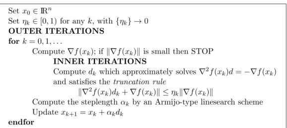
Table 4.1: The linesearch-based truncated Newton method we adopted. Set 𝑥0 ∈ IR𝑛

Set 𝜂𝑘∈ [0, 1) for any 𝑘, with {𝜂𝑘} → 0 OUTER ITERATIONS

for 𝑘 = 0, 1, . . .

Compute ∇𝑓 (𝑥𝑘); if ∥∇𝑓 (𝑥𝑘)∥ is small then STOP INNER ITERATIONS

Compute 𝑑𝑘 which approximately solves ∇2𝑓 (𝑥𝑘)𝑑 = −∇𝑓 (𝑥𝑘) and satisfies the truncation rule

∥∇2𝑓 (𝑥𝑘)𝑑𝑘+ ∇𝑓 (𝑥𝑘)∥ ≤ 𝜂𝑘∥∇𝑓 (𝑥𝑘)∥

Compute the steplength 𝛼𝑘 by an Armijo-type linesearch scheme Update 𝑥𝑘+1= 𝑥𝑘+ 𝛼𝑘𝑑𝑘

0 10 20 30 40 50 0 0.2 0.4 0.6 0.8 1 1.2 1.4 1.6 1.8 2x 10 9 Unprecond Precond (h1) 0 10 20 30 40 50 0 0.2 0.4 0.6 0.8 1 1.2 1.4 1.6 1.8 2x 10 9 Unprecond Precond (h2) 0 10 20 30 40 50 0 0.2 0.4 0.6 0.8 1 1.2 1.4 1.6 1.8 2x 10 9 Unprecond Precond (h3) 0 10 20 30 40 50 0 0.2 0.4 0.6 0.8 1 1.2 1.4 1.6 1.8 2x 10 9 Unprecond Precond (h4) 0 10 20 30 40 50 0 0.2 0.4 0.6 0.8 1 1.2 1.4 1.6 1.8 2x 10 9 Unprecond Precond (h5)

Figure 4.7: Comparison between the full spectra Λ[𝐴0] (Unprecond) and Λ[𝑀_ℎ♯(0, 1, 𝐼)𝐴0] (Precond), with 𝐴0 nonsingular (eigenvalues are sorted for simplicity); we used different values of ℎ (ℎ1 = 4, ℎ2 = 8, ℎ3 = 12, ℎ4 = 16, ℎ5 = 20). The eigenvalues in the spectrum Λ[𝑀_ℎ♯(0, 1, 𝐼)𝐴0] are in general smaller than the corresponding eigenvalues in Λ[𝐴0]. The eigenvalues in Λ[𝑀_ℎ♯(0, 1, 𝐼)𝐴0] are also more clustered near +1. The starting point of the CG is 𝑥0= 0.

0 10 20 30 40 50 0 0.2 0.4 0.6 0.8 1 1.2 1.4 1.6 1.8 2x 10 9 Unprecond Precond (h1) 0 10 20 30 40 50 0 0.2 0.4 0.6 0.8 1 1.2 1.4 1.6 1.8 2x 10 9 Unprecond Precond (h2) 0 10 20 30 40 50 0 0.2 0.4 0.6 0.8 1 1.2 1.4 1.6 1.8 2x 10 9 Unprecond Precond (h3) 0 10 20 30 40 50 0 0.2 0.4 0.6 0.8 1 1.2 1.4 1.6 1.8 2x 10 9 Unprecond Precond (h4) 0 10 20 30 40 50 0 0.2 0.4 0.6 0.8 1 1.2 1.4 1.6 1.8 2x 10 9 Unprecond Precond (h5)

Figure 4.8: Comparison between the full spectra Λ(𝐴0) (Unprecond) and Λ[𝑀_ℎ♯(0, 1, 𝐼)𝐴0] (Precond), with 𝐴0 nonsingular (eigenvalues are sorted for simplicity); we used different values of ℎ (ℎ1 = 4, ℎ2 = 8, ℎ3 = 12, ℎ4 = 16, ℎ5 = 20). The eigenvalues in the spectrum Λ[𝑀_ℎ♯(0, 1, 𝐼)𝐴0] are in general smaller than the corresponding eigenvalues in Λ[𝐴0]. The eigenvalues in Λ[𝑀_ℎ♯(0, 1, 𝐼)𝐴0] are also more clustered near +1. The starting point of the CG is 𝑥0= 100𝑒.

0 5 7 9 11 13 15 17 19 21 −5 0 5 10x 10 10 Cond(A) Cond(M−1A)

Figure 4.9: The condition number of matrix 𝐴1 (𝐶𝑜𝑛𝑑(𝐴)) along with the condition number of matrix 𝑀_ℎ♯(0, 1, 𝐼)𝐴1 (𝐶𝑜𝑛𝑑(𝑀−1𝐴)), when 4 ≤ ℎ ≤ 20. The condition number of 𝐴1 is now slightly smaller than the condition number of 𝑀_ℎ♯(0, 1, 𝐼)𝐴1, for any value of the parameter ℎ. The starting point of the CG is 𝑥0 = 0.

iteration 𝑘 we computed the preconditioner 𝑀_ℎ♯(𝑎, 1, 𝐼), with ℎ ∈ {4, 8, 12, 16, 20}, by using the CG to solve the equation ∇2_{𝑓 (𝑥}

𝑘)𝑑 = −∇𝑓 (𝑥𝑘). Then, we adopted 𝑀_ℎ♯(0, 1, 𝐼) as a preconditioner for the solution of Newton’s equation of the subsequent iteration

∇2𝑓 (𝑥𝑘+1)𝑑 = −∇𝑓 (𝑥𝑘+1).

The iteration index 𝑘 was randomly chosen, in such a way that ∥𝑥𝑘+1 − 𝑥𝑘∥ was small

(i.e. the entries of the Hessian matrices ∇2_{𝑓 (𝑥}

𝑘) and ∇2𝑓 (𝑥𝑘+1) are not expected to differ significantly). For simplicity we just report the results on two test problems, using 𝑛 = 1000, in the set of all the optimization problems experienced. Very similar results were obtained for almost all the test problems. In Figures 4.13-4.14 we consider the problem NONCVXUN; without loss of generality we only show the numerical results for ℎ = 16. Observe that since 𝑥𝑘+1is close to 𝑥𝑘(i.e. we are eventually converging to a local minimum) the Hessian matrix ∇2_{𝑓 (𝑥}

𝑘+1) is positive semidefinite. Furthermore, again the eigenvalues larger than +1 in Λ[∇2𝑓 (𝑥𝑘+1)] are scaled in Λ[𝑀_ℎ♯(0, 1, 𝐼)∇2𝑓 (𝑥𝑘+1)]. Similarly we show in Figures 4.15-4.16 the results for the test function NONDQUAR in CUTEr collection. The test problems in this optimization framework, where the preconditioner 𝑀_ℎ♯(0, 1, 𝐼) is computed at the outer iteration 𝑘 and used at the outer iteration 𝑘 + 1, confirm that the properties of Theorem 2.1 may hold also when 𝑀_ℎ♯(0, 1, 𝐼) is used on a sequence of linear systems 𝐴𝑘𝑥 = 𝑏𝑘, when 𝐴𝑘 changes slightly with 𝑘.

0 5 7 9 11 13 15 17 19 21 −1 0 1 2 3 4 5x 10 9 Cond(A) Cond(M−1A)

Figure 4.10: The condition number of matrix 𝐴1 (𝐶𝑜𝑛𝑑(𝐴)) along with the condition num-ber of matrix 𝑀_ℎ♯(0, 1, 𝐼)𝐴1 (𝐶𝑜𝑛𝑑(𝑀−1𝐴)), when 4 ≤ ℎ ≤ 20. The condition number of 𝐴1 is now slightly larger than the condition number of 𝑀_ℎ♯(0, 1, 𝐼)𝐴1, for any value of the parameter ℎ. The starting point of the CG is 𝑥0 = 100𝑒.

5

Conclusions

We have given theoretical and numerical results for a class of preconditioners, which are parameter dependent. The preconditioners can be built by using any Krylov subspace method for the symmetric linear system (2.1), provided that it is able to satisfy the general conditions (2.2)-(2.3) in Assumption 2.1. The latter property may be appealing in several real problems, where a few iterations of the Krylov subspace method adopted may suffice to compute an effective preconditioner.

Our proposal seems tailored also for those cases where a sequence of linear systems of the form

𝐴𝑘𝑥 = 𝑏𝑘, 𝑘 = 1, 2, . . .

requires a solution (e.g., see [12] for details), where 𝐴𝑘 slightly changes with the index 𝑘. In the latter case, the preconditioner 𝑀_ℎ♯(𝑎, 𝛿, 𝐷) in (2.4)-(2.5) can be computed applying the Krylov subspace method to the first linear system 𝐴1𝑥 = 𝑏1. Then, 𝑀_ℎ♯(𝑎, 𝛿, 𝐷) can be used to efficiently solve 𝐴𝑘𝑥 = 𝑏𝑘, with 𝑘 = 2, 3, . . .

Finally, the class of preconditioners in this paper seems a promising tool also for the solution of linear systems in financial frameworks. In particular, we want to focus on symmetric linear systems arising when we impose KKT conditions in portfolio optimization problems, with a large number of titles in the portfolio, along with linear equality constraints [2].

0 20 40 60 80 100 120 140 160 180 0 2 4 6 8 10 12 14x 10 7 Unprecond Precond (h1) 0 20 40 60 80 100 120 140 160 180 0 2 4 6 8 10 12 14x 10 7 Unprecond Precond (h2) 0 20 40 60 80 100 120 140 160 180 0 2 4 6 8 10 12 14x 10 7 Unprecond Precond (h3) 0 20 40 60 80 100 120 140 160 180 0 2 4 6 8 10 12 14x 10 7 Unprecond Precond (h4) 0 20 40 60 80 100 120 140 160 180 0 2 4 6 8 10 12 14x 10 7 Unprecond Precond (h5)

Figure 4.11: Comparison between the full spectra Λ[𝐴1] (Unprecond) and Λ[𝑀ℎ♯(0, 1, 𝐼)𝐴1] (Precond); the eigenvalues are sorted for simplicity). We used different values of ℎ (ℎ1 = 4, ℎ2 = 8, ℎ3 = 12, ℎ4 = 16, ℎ5 = 20). Again, the eigenvalues in the spectrum Λ[𝑀_ℎ♯(0, 1, 𝐼)𝐴1] are in general smaller than the corresponding eigenvalues in Λ[𝐴1]. The eigenvalues in Λ[𝑀_ℎ♯(0, 1, 𝐼)𝐴1] are more clustered near +1. The starting point of the CG is 𝑥0 = 0.

0 20 40 60 80 100 120 140 160 180 0 2 4 6 8 10 12 14x 10 7 Unprecond Precond (h1) 0 20 40 60 80 100 120 140 160 180 0 2 4 6 8 10 12 14x 10 7 Unprecond Precond (h2) 0 20 40 60 80 100 120 140 160 180 0 2 4 6 8 10 12 14x 10 7 Unprecond Precond (h3) 0 20 40 60 80 100 120 140 160 180 0 2 4 6 8 10 12 14x 10 7 Unprecond Precond (h4) 0 20 40 60 80 100 120 140 160 180 0 2 4 6 8 10 12 14x 10 7 Unprecond Precond (h5)

Figure 4.12: Comparison between the full spectra Λ[𝐴1] (Unprecond) and Λ[𝑀ℎ♯(0, 1, 𝐼)𝐴1] (Precond); the eigenvalues are sorted for simplicity. We used different values of ℎ (ℎ1 = 4, ℎ2 = 8, ℎ3 = 12, ℎ4 = 16, ℎ5 = 20). Again, the eigenvalues in the spectrum Λ[𝑀_ℎ♯(0, 1, 𝐼)𝐴1] are in general smaller than the corresponding eigenvalues in Λ[𝐴1]. The eigenvalues in Λ[𝑀_ℎ♯(0, 1, 𝐼)𝐴1] are more clustered near +1. The starting point of the CG is 𝑥0 = 100𝑒.

0 2 4 6 8 10 12 14 16 18 0 1 2 3 4 5 6x 10 18 Cond(A) Cond(M−1A)

Figure 4.13: The condition number of matrix ∇2_{𝑓 (𝑥}

𝑘+1) (𝐶𝑜𝑛𝑑(𝐴)) along with the condi-tion number of matrix 𝑀_ℎ♯(0, 1, 𝐼)∇2_{𝑓 (𝑥}

𝑘+1) (𝐶𝑜𝑛𝑑(𝑀−1𝐴)), for the optimization problem

NONCVXUN, when 1 ≤ ℎ ≤ 17. The condition number of ∇2_{𝑓 (𝑥}

𝑘+1) is nearby the condi-tion number of 𝑀_ℎ♯(0, 1, 𝐼)∇2_{𝑓 (𝑥}

𝑘+1), for any value of the parameter ℎ. The value 𝑘 = 175 was the first step such that ∥𝑥𝑘+1 − 𝑥𝑘∥ ≤ 10−3∥𝑥𝑘∥ (i.e. 𝑥𝑘+1 and 𝑥𝑘 are sufficiently close) and 𝛼𝑘 ≥ 0.95 (i.e. we are likely close to the minimum point). In particular it was ∥𝑥175− 𝑥176∥ ≈ 0.083.

0 200 400 600 800 1000 −5 0 5 10 15 20 25 30 35 40 Unprecond Precond (h4) 0 50 100 150 200 −1.5 −1 −0.5 0 0.5 1 1.5 2 Unprecond Precond (h4)

Figure 4.14: Comparison between the full spectra/detailed spectra (left figure/right figure) of ∇2_{𝑓 (𝑥}

𝑘+1) (Unprecond) and 𝑀_ℎ♯(0, 1, 𝐼)∇2𝑓 (𝑥𝑘+1) (Precond), for the optimization problem NONCVXUN, with ℎ = ℎ4 = 16. The eigenvalues in Λ[𝑀_ℎ♯(0, 1, 𝐼)∇2_{𝑓 (𝑥}

𝑘+1)] larger than +1 are evidently attenuated, so that Λ[𝑀_ℎ♯(0, 1, 𝐼)∇2𝑓 (𝑥𝑘+1)] is more clustered.

References

[1] MATLAB Release 2011a, The MathWorks Inc., 2011.

[2] G. Al-Jeiroudi, J. Gondzio, and J. Hall, Preconditioning indefinite systems in interior point methods for large scale linear optimisation, Optimization Methods & Software, 23 (2008), pp. 345–363.

[3] T. Belytschko, A. Bayliss, C. Brinson, S. Carr, W. Kath, S. Krishnaswamy, and B. Moran, Mechanics in the engineering first curriculum at Northwestern Uni-versity, Int. J. Engng. Education, 13 (1997), pp. 457–472.

[4] D. S. Bernstein, Matrix Mathematics: Theory, Facts, and Formulas (Second Edi-tion), Princeton University Press, Princeton, 2009.

[5] G. Fasano, Planar–conjugate gradient algorithm for large–scale unconstrained op-timization, Part 1: Theory, Journal of Optimization Theory and Applications, 125 (2005), pp. 523–541.

[6] G. Fasano and M. Roma, A class of preconditioners for large indefinite linear sys-tems, as by-product of Krylov subspace methods: Part 1, Technical Report n. 4, De-partment of Management, University Ca’Foscari, Venice, Italy, 2011.

[7] S. Geman, A limit theorem for the norm of random matrices, The Annals of Proba-bility, 8 (1980), pp. 252–261.

0 2 4 6 8 10 12 14 16 18 2 4 6 8 10 12 14 16 18x 10 10 Cond(A) Cond(M−1A)

Figure 4.15: The condition number of matrix ∇2_{𝑓 (𝑥}

𝑘+1) (𝐶𝑜𝑛𝑑(𝐴)) along with the condi-tion number of matrix 𝑀_ℎ♯(0, 1, 𝐼)∇2_{𝑓 (𝑥}

𝑘+1) (𝐶𝑜𝑛𝑑(𝑀−1𝐴)), for the optimization problem

NONDQUAR, when 1 ≤ ℎ ≤ 17. The condition number of ∇2_{𝑓 (𝑥}

𝑘+1) is now slightly larger than the condition number of 𝑀_ℎ♯(0, 1, 𝐼)∇2_{𝑓 (𝑥}

𝑘+1) (though they are both ≈ 1010). The value 𝑘 = 40 was the first step such that ∥𝑥𝑘+1− 𝑥𝑘∥ ≤ 10−3∥𝑥𝑘∥ (i.e. 𝑥𝑘+1 and 𝑥𝑘 are suf-ficiently close) and 𝛼𝑘≥ 0.95 (i.e. we are likely close to the minimum point). In particular it was ∥𝑥40− 𝑥41∥ ≈ 0.203.

0 200 400 600 800 1000 −30 −20 −10 0 10 20 30 40 Unprecond Precond (h4) 0 2 4 6 8 10 −35 −30 −25 −20 −15 −10 −5 0 5 10 15 20 Unprecond Precond (h4) 975 980 985 990 995 1000 1005 −0.5 0 0.5 1 1.5 2 2.5 3 3.5 4 4.5 5 Unprecond Precond (h4)

Figure 4.16: Comparison between the full spectra/detailed spectra (upper figure/lower fig-ures) Λ[∇2𝑓 (𝑥𝑘+1)] (Unprecond) and Λ[𝑀ℎ−1∇2𝑓 (𝑥𝑘+1)] (Precond), for the optimization problem NONDQUAR, with ℎ = ℎ4 = 16. Some nearly-zero eigenvalues in the spectrum Λ[∇2𝑓 (𝑥𝑘+1)] are shifted to non-zero values in Λ[𝑀ℎ♯(0, 1, 𝐼)∇2𝑓 (𝑥𝑘+1)]. Since many eigen-values in Λ[∇2𝑓 (𝑥𝑘+1)] are zero or nearly-zero, the preconditioner 𝑀ℎ♯(0, 1, 𝐼) may be of scarce effect, unless large values of the parameter ℎ are considered.

[8] P. E. Gill, W. Murray, D. B. Poncele´on, and M. A. Saunders, Preconditioners for indefinite systems arising in optimization, SIAM J. Matrix Anal. Appl., 13 (1992), pp. 292–311.

[9] G. Golub and C. Van Loan, Matrix Computations, The John Hopkins Press, Bal-timore, 1996. Third edition.

[10] N. I. M. Gould, D. Orban, and P. L. Toint, CUTEr (and sifdec), a constrained and unconstrained testing environment, revised, ACM Transaction on Mathematical Software, 29 (2003), pp. 373–394.

[11] C. Lanczos, An iteration method for the solution of the eigenvalue problem of linear differential and integral, J. Res. Nat. Bur. Standards, 45 (1950), pp. 255–282.

[12] J. Morales and J. Nocedal, Automatic preconditioning by limited memory quasi– Newton updating, SIAM Journal on Optimization, 10 (2000), pp. 1079–1096.

[13] S. Nash, A survey of truncated-Newton methods, Journal of Computational and Ap-plied Mathematics, 124 (2000), pp. 45–59.

[14] J. Nocedal and S. Wright, Numerical Optimization (Springer Series in Operations Research and Financial Engineering) - Second edition, Springer, New York, 2000. [15] C. Paige and M. Saunders, Solution of sparse indefinite systems of linear equations,

SIAM Journal on Numerical Analysis, 12 (1975), pp. 617–629.

[16] Y. Saad, Iterative Methods for Sparse Linear Systems, Second Edition, SIAM, Philadelphia, 2003.