Contents
1 Introduction 3
1.1 Experimental Evidence . . . 3
1.2 DM candidates . . . 4
1.3 This thesis . . . 5
2 WIMP’s relic abundance 7 2.1 Decoupling . . . 7
2.2 Boltzmann equation . . . 8
2.3 Temperature averaged cross section . . . 9
2.4 Solving the Boltzmann equation . . . 9
2.5 Relic abundance . . . 10
3 Two special cases 13 3.1 Coannihilation . . . 13
3.1.1 Coannihilation Cross Sections . . . 14
3.2 Annihilation into ”forbidden” channels . . . 15
4 The model 17 4.1 Mass Spectrum . . . 17
4.2 Interactions . . . 18
4.2.1 Interctions with scalar particles . . . 18
4.2.2 Interactions with Gauge Bosons . . . 21
4.3 EWPT . . . 23
5 Important Cross Sections 27 5.1 Annihilation cross section . . . 27
5.1.1 mL < mW . . . 27
5.1.2 mL > mW . . . 28
5.1.3 mL ∼ mW . . . 30
5.2 Detection cross section . . . 31 1
2 CONTENTS 6 Relic Abundances 33 6.1 mL. mW . . . 33 6.1.1 mL< mW . . . 33 6.1.2 mLv mW . . . 34 6.1.3 mL. mW . . . 34 6.2 mL> mW . . . 36
7 Summary and Conclusions 37 7.1 Collider signals . . . 37
7.2 Conclusions . . . 38
Chapter 1
Introduction
There are several experimental evidences that suggest that most of the matter of the Universe does not shine and that it is not even barionic. One of the most important issues in particle physics is finding out what the so called Dark Matter (DM) is made of. Although the argument is far away to be settled, there are few features of DM on which there is some agreement. The first is that it must not couple to photons, otherwise it would not be dark. Another feature of DM is that it should be stable and weakly interacting, otherwise we could not explain its observed mass density. It should also be classical, in a sense that we do not bother wheter it is fermionic or bosonic as we study it with Boltzmann statistics. From Large Scale Structure formation it was inferred that it should also be cold. We will now briefly review the experimental evidence for DM and then recall some of the particles that have been proposed as DM candidates before going on.
1.1
Experimental Evidence
The most compelling evidence for the existence of Dark Matter on galactic scales comes from the observations of the rotation curves of spiral galaxies, that is the graph of circular velocities of stars and gases as a function of their distances from the galactic center.
In Newtonian dynamics we expect the circular velocity to be
v(r) =
r
GM(r)
r (1.1)
where M(r) = 4πR ρ(r)r2dr and ρ(r) is the mass density profile. We ex-pected v to fall as √1
r beyond the optical disk. But v is found to be constant
4 CHAPTER 1. INTRODUCTION
by experiments, so a problem arose: there is not enought luminous mat-ter observed in spiral galaxies to account for their observed rotation curves. This could be explained either by dominant quantities of non luminous Dark Matter or by a modified gravitational law.
Many works that tried to distinguish between the two alternatives were based on nontrivial assumptions that left room to doubts. The existence of DM could only be confirmed either by laboratory detection or, in astronom-ical context, by the discovery of a system in which the observed barions and the inferred DM are spatially separated. In such a case no trivial assump-tions, such as symmetry or the location of the center of mass system are needed.
Such a system has recently been seen in the unique cluster 1E0657 − 558. During a merger of two cluster, galaxies behave as collisionless particles, while the fluid-like X-ray emitting intracluster plasme experiences pressure. The observed displacement between the bulk of the barions and the gravita-tional potential proved the presence of DM for the most general assumptions regarding the behaviour of gravity [?].
1.2
DM candidates
Many particles have been proposed as dark matter candidates. We want here to racall briefly only two of them: the lightest supersymmetric particle and the scalar singlet. The first because it is perhaps the most well motivated and the most well developed WIMP, the other because it is the easiest extension of Standard Model (SM) that accounts for for Dark Matter and because it is strictly related to the model on which we will focus later on in this thesis.
Lightest Supersymmetric particle. Supersymmetric (SUSY) extension of
the SM naturally predict the existence of DM candidates which is the Light-est Supersymmetric Particle (LSP). In Supersymmetric theories there is a symmetry, called R parity, that is conserved. SM particles are even under
R parity, while their supersymmetric partners are odd. The conservation of
this symmetry makes the LSP a massive, stable and weak interacting parti-cle, that is a perfect DM candidate. The LSP may be the neutralino or the gravitino, whichever is the lightest. The neutralinos are Majorana fermions resulting from the linearcombination of the neutral components of the Hig-gsino, the Photino and the Zino. Those particles, which are respectively the supersymmetric partners of the Higgs, the photon and the Z are in fact not masses eigenstates. The gravitino is the spin 3
2 superpartner of the graviton in supergravity theories. It gets nonvanishing mass after spontaneous sym-metry breaking of local supersymsym-metry. However gravitinos are very difficult
1.3. THIS THESIS 5 to observe.
Scalar Singlet The Scalar Singlet is the simplest extension of SM
com-patible with DM. We recall it here because the model we will analize later on is the second simplest. The model consists in adding to SM a Real Scalar Singlet. It is coupled only to Higgs boson because, being a singlet, it has no gauge couplings. If its mass is smaller than 2 Higgs masses it cannot decay, so it is stable. Many people studied this DM candidate but it is not jet clear whether or not it is a suitable DM candidate.
1.3
This thesis
The purpose of this thesis is to study in some detail the case of a model of DM which involves a neutral scalar particle. This particle arises in a minimal extension of the SM by including a second Higgs doublet with a positive m2 and, as such, does not get a vacuum expectation value (vev).
To avoid the coupling of this doublet to fermions, which might lead to problems in flavour physics, it is required to the lagrangian to be invariant under H2 → −H2. This and the fact that H2 does not get a vev makes the lightest of the scalars that compose H2 (2 neutral and one charged particle) stable and therefore a candidate for DM.
In chapter 2 we will derive the standard formula used to calculate relic abundances of particles species, in chapter 3 we will analise two special case in which the standard formula fails to predict the correct relic abundance, and we will show how the standard formula should be modified in each case. In chapter 4 we present the model on which we will focus. In chapter 5 we will compute the cross section important for direct detection of the particle and the cross sections which we will use in chapter 6 to calculate relic abun-dance of the lightest particle belonging to the doublet. In chapter 7, before conclusions, we make a brief comment on the possibility of finding signals of those particles at colliders.
Chapter 2
WIMP’s relic abundance
Once a particle species totally decouples from the thermal plasma its evo-lution is very simple: its number density decreases as R−3[?]. What is not
simple at all is the evolution of the particle species around the epoch of the decoupling. We will derive the equations that describe the behaviour of particles of a species around the epoch of decoupling starting from their Boltzmann equation. Given those equations we can easily figure out the relic abundance of the particles species we are analizing.
2.1
Decoupling
First we have to explain what we mean by decoupling. We say that a par-ticle species decopled from thermal plasma when the interaction rate of the particle species becomes smaller than the expansion rate of the Universe or
Γ . H (2.1)
where Γ is the interaction rate per particle for the reaction (or the reactions) that keeps the species in thermal equilibrium and H = ˙a
a is the Hubble
costant, a is the scale factor and ˙a its derivative with respect to time. The very moment in which particles cease to interact with thermal plasma is called freeze out. (2.1) is a very useful rule, often very accurate in its predictions, but if we want to treat in detail the decoupling we must follow the microscopic evolution of every particle’s phase space distribution function
f (xµ, pµ), which is governed by the Boltzmann equation.
8 CHAPTER 2. WIMP’S RELIC ABUNDANCE
2.2
Boltzmann equation
We are interested in the relic abundance of a particle species ψ that we assume stable, so that the most important way to change their abundance is through annihilation into other particles species:
ψ ¯ψ ↔ ϕiϕ¯i (2.2)
where ϕi are all the possible particles into which our relic can annichilate.
We assume the ϕis in thermal equilibrium.
The Boltzmann equation for our problem is then
dnψ
dt + 3Hnψ = − < σA|v| > [n
2
ψ − (nEQϕ )2]
where < σA|v| > is the thermally averaged total annichilation cross section
times the velocity, nψ is the actual number of ψs particles and nEQϕ is the
number of ϕs particles at thermal equilibrium. Since nEQ ∝ exp[−E/kT ],
for any particle of given energy E, by energy conservation we find (nEQ ϕ )2 =
(nEQψ )2 so that the previous equation can be rewritten as
dnψ
dt + 3Hnψ = − < σA|v|n
2
ψ− (nEQψ )2] (2.3)
The 3Hnψ term accounts for the variation in the number density of ψ
par-ticles due to the expanding Universe while the right hand side of equation (2.3) accounts for the destruction rate of ψ particles.
It is convenient to eliminate the explicit dependence on the Universe expansion. This can be achieved using Y = nψ/s, the number of particles
per unit of comoving volume1, instead of n
ψ as variable in (2.3). With this
change of variables the equation becomes ˙
Y = −hσA|v|i[Y2− Yeq2] (2.4)
where the dotted Y means the derivative of Y with respect to time and Yeq is
the number of particles per unit comoving volume at thermal equilibrium. It is also useful to introduce the dimensionless variable x = mψ/T where mψ is
the mass of the particle and T is the thermal plasma temperature, connected to the time t in the usual way. With respect with this new variable Yeq can
be written as
Yeq ∝ x3/2e−x (2.5)
2.3. TEMPERATURE AVERAGED CROSS SECTION 9
2.3
Temperature averaged cross section
We are interested in the relic abundance of massive particles. As these par-ticles have non zero mass, they would be non relativistic by the time of their freeze out. In this non relativistic situation total annihilation cross section times the velocity should have a velocity dependance: σA|v| ∝ vp with p = 0
in case of s-wave annihilation, p = 2 in case of p-wave annihilation and so on. As hvi ∝ T1/2, we can parametrise the total annihilation cross section times the velocity dependance from temperature as hσA|v|i ∝ Tnwith n = 0
for s-wave annihilation, n = 1 for p-wave annihilation and so on. Therefore we have hσA|v|i ≡ σ0( T m) n= σ 0x−n (2.6)
2.4
Solving the Boltzmann equation
It is possible to rewrite equation (2.4) in terms of the Y derivative with respect to x dY dx = − λ xn+1(Y 2− Y2 eq) (2.7) where λ = h hσA|v|is H i
To understand the solution of this equation in an approx-imate analytic way, one argue as follows. λ is a function of x which becomes approximately 1 at xf. This happens when the Boltzmann factor suppresses
the interaction rate, i.e. at xf significantly grater than 1. Tf = mxfψ is the ”freeze out temperature”. When x ¿ xf we have
dY dx ∼ Y x λ xn+1 À 1 (2.8)
so to satisfy equation (2.7) it should be Y2− Y2
eq ∼ 0 that is Y ∼ Yeq. This
means that very long before freeze out Y tracks Yeq.
When x À xf we have
λ
xn+1 ¿ 1 (2.9)
so from equation (2.7) it is dY
dx ∼ 0. Very long after freeze out Y is a
constant function of x except for the reduction in particle’s number due to coannihilation . We need an expression to describe Y in this region
Y∞=
(n + 1)xn f
10 CHAPTER 2. WIMP’S RELIC ABUNDANCE
The subscript ∞ stands for final abundance which is the asimptotic particle number per unit comoving volume we need in order to compute the particles abundance nowadays.
We want to find the point xf where Y ceases to track Yeq and becomes
constant. By numerical means we find an expression for xf
xf w ln[0.038(n + 1)(g/g∗1/2)mP lmψσ0] (2.11) where g is defined as the number of degrees of freedom of ψ (2 if a Majorana fermion, 1 if a neutral scalar ) and g∗is the total number of degrees of freedom
of the relativistic particles present in the thermal plasma at freeze out, mP l
is the Planck mass and mψ is the particles mass.
2.5
Relic abundance
Once we have Y∞ it is straightforward to find nψ0 = s0Y∞
= 1.13 × 10⁴ (n + 1)x
n+1
(g∗S/g1/2∗ )mP lmψσ0
cm−3 (2.12) where s0 is the present entropy density and g∗S is tne number of
relativis-tic degrees of freedom that enter the entropy density expression The relic abundance for our particle species is then
Ωψh2 = %ψ %c h2 = mψnψ0 %c h2 = 0.035 × (n + 1)x n+1 f (g∗S/g∗1/2)σ0(pb) . (2.13)
If we take g∗ = g∗S, that is well verified assumption until freeze out,
equation (2.13) can be written as
Ωh2 = 0.034
g∗1/2J(pb)
(2.14) where we have included a better approximation through a suitably averaged cross section in J (xf) = Z ∞ xf hσvi x2 dx (2.15) and xf = ln 0.038gmP lmψhσvi g∗1/2x1/2f (2.16)
2.5. RELIC ABUNDANCE 11 For a typical weak interaction cross section and mψ = O(100GeV ), xf ' 20
(see chapter 6), so that at T∗ = O(1 ÷ 10GeV ) g
∗ ' O(10 − 100). The
theoretical value of Ωh2 in equation (2.14) should be compared with the observed value by experiments in cosmology, Ωh2 = 0.09 ÷ 0.12.
Chapter 3
Two special cases
The formulas we have just derived apply in general cases. In a few cases those formulas can fail to give the correct predictions by a factor two or more and we have to apply more detailed formulas if we want the correct prediction [?]. There are two cases of particular interest for our following purposes: the first is the case when cohannihilation is as important as annihilation in the reduction in particle number, the other case is when relic particles annihilate into particles more massive than relic particles themselves.
3.1
Coannihilation
We call coannihilation a process like this
L + NL → X + X0 (3.1)
where L and NL have similar masses and X and X0 are two SM particles.
To be a suitable dark matter candidate, the lightest of those particles must be protected by a simmetry that makes it stable. Since L (L stands for lightest) cannot decay, the only way to reduce its abundance is throught annihilation into other SM particles.
This is true unless L and NL (NL stands for Next to Lightest) are nearly degenerate in mass, so that
mN L− mL= ∆m ¿ mN L, mL (3.2)
In this case the coannihilation of lightest with next to lightest into other particles becomes as important as annihilation in describing the reduction in the number of lightest particles. We have to include coannihilations into the Boltzmann equation (2.3) to have correct predictions for the relic abundance.
14 CHAPTER 3. TWO SPECIAL CASES
3.1.1
Coannihilation Cross Sections
Our aim is to include coannihilations into Boltzmann equation (2.3) without changing its form, so that we can solve it in the same way we did in the previous chapter.
We define an effective cross section as
σef f = 2σN L−LgLgN L g2 ef f (1 + ∆)32exp(−x∆) + +σN L−N Lg 2 N L g2 ef f (1 + ∆)3exp(−2x∆) + σL−L (3.3) where gef f = g(1 + ∆)3/2exp(−x∆) (3.4)
is the effective number of degrees of freedom, gL is the number of degrees of
freedom of the lightest particle, gN L is the number of degrees of freedom of
the next to lightest particle and
∆ = mN L− mL
mL
. (3.5)
σL−L is the annihilation cross section of L into standard model particles, σN L−N Lis the annihilation cross section of NL into standard model particles
and σL−N L in the coannihilation cross section of L and NL into standard
model particles.
Now the Boltzmann equation (2.3) can be cast in the form
dn
dt + 3Hn = − < σef fv > [n
2− n2
eq] (3.6)
that is exactly the same form of the expression for which we found the gen-eral solution (2.3) in the previous chapter. Of course, as σv can be Taylor expanded as σv = a + bv2 , also σ
ef f can be Taylor expanded, and it becomes σef f = aef f + bef fv2.
The expression for xf is the same as (2.16) except for the obvios changing
in the names of the variables:
xf = ln
0.038gef fmP lmLhσef fvi g∗1/2x1/2f
(3.7) The annihilation integral (2.15) becomes
J = Ia+
3Ib
xf
3.2. ANNIHILATION INTO ”FORBIDDEN” CHANNELS 15 where Ia = xf Z ∞ xf aef f x2 dx Ib = 2x 2 f Z ∞ xf bef f x3 dx (3.9) Ωh2 is the same as in equation (2.14) but with J found in equation (3.8):
Ωh2 = 0.035
g12 ∗J(pb)
(3.10)
3.2
Annihilation into ”forbidden” channels
A reaction whose products are heavier than the initial particles at rest is forbidden by cinematics. However it can happen if there is sufficient ther-mal energy. Therther-mal energy effectively lowers the threshold energy of the reaction. In such a case we cannot assume that the outgoing particles are massless because, since we are very close to threshold, their masses cannot be neglected.
Let us consider the case in which the annihilation cross section is pre-dominantly in s − wave, so that hσvi = av2 where v2 is the velocity of the final particle in the center of mass system. We define
µ = |1 − z2|1/2
z z =
mf
mi (3.11)
where mi and mf are the masses of the initial and final particle respectively.
In terms of those variables, the thermal average of the cross section can be written as hσvi =< a0v2 >= a0 µ −2zx1/2 π1/2 exp(±µ − 2x/2) K 1(µ −2 x/2) (3.12) where K1 is the modified Bessel function. The ± sign is respectively for the case in which one is above or below threshold for the reaction at rest.
Chapter 4
The model
Our model introduces in the Standard Model a new scalar doublet H2 with the same quantum numbers of the standard Higgs doublet but which does not get a vacuum expectation value [?]. Because of this reason, to distinguish it from the standard Higgs doublet, we refer to it as ”inert” doublet. In order to make this scalar doublet non-interacting directly with fermions we introduce a Z2 symmetry:
H2 → −H2 (4.1)
This symmetry prevents the lightest component of the scalar doublet from decaing, making it a suitable dark matter candidate.
4.1
Mass Spectrum
The most general scalar potential that describes the interactions of this dou-blet is: V = µ2 1|H1|2+ µ22|H2|2+ λ1|H1|4+ λ2|H2|4+ λ3|H1|2|H2|2+ +λ4|H1†H2|2+ λ5 2 ·³ H1†H2 ´2 + h.c. ¸ (4.2) where H1is the Standard Model Higgs doublet. The doublets are parametrized in terms of the physical fields as follows:
H1 = µ φ+ v + h+ıχ√ 2 ¶ H2 = µ H+ S+ıA√ 2 ¶ (4.3) As usual the Goldstone bosons φ+ and χ can be set to zero when we choose the unitary gauge. The inert scalar doublet is made of three physical parti-cles, one charged particle, H+ and two neutral particles, S and A. The mass
18 CHAPTER 4. THE MODEL
spectrum of the physical particles of the inert doublet is :
m2
I = µ22+ λIv2, I = {H, S, A}
λH = λ3 (4.4)
λS = λ3+ λ4+ λ5
λA = λ3+ λ4− λ5
v is the SM Higgs vev and v = 175GeV .
The bounds on dark matter abundance tell us that the lightest particle, to become a suitable dark matter candidate should not be charged, so the lightest particle L should either be A or S. Furthermore, for the consistency with the Electroweak Precision Tests H should be heavier than both A and
S. Therefore the next to lightest particle, NL, will also be neutral, with mH > mN L ≥ mL. From the previous formula this means λH > λS,A,
which can be rewritten in terms of the coupling constants in the interaction lagrangian as λ4 > |λ5|.
We want our potential to be bounded from below. The prescription on the parameters to ensure this is
λ1, λ2 > 0 λ3, λL≡ λ3+ λ4− |λ5| > −2 p
λ1λ2 (4.5) In the following we shall put
λ2 . 1 (4.6)
to avoid any problem with perturbativity.
4.2
Interactions
4.2.1
Interctions with scalar particles
Inserting in the scalar potential (4.2) the parametrization of the fields (4.3) we find how the physical particles belonging to the inert doublet interact with particles belonging to the Higgs doublet.
The quadratic interactions give their contribution only to the masses of the particles, as it is shown in the particles mass spectrum (4.4).
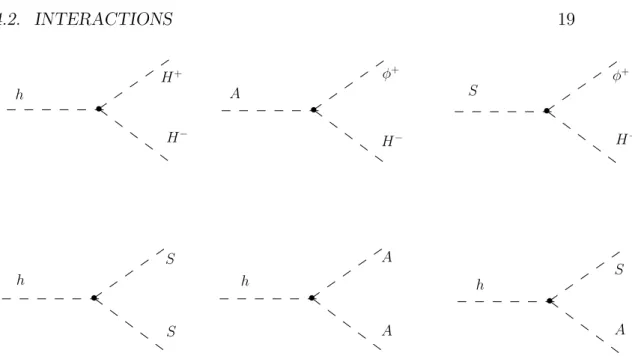
The cubic interactions are:
Vc = v × ( √ 2λ3H+H−h + λ3+ λ√4+ λ5 2 hSS + λ3+ λ√4− λ5 2 hAA + + · λ4√+ λ5 2 φ −H+S + h.c ¸ + · ı(λ4√− λ5) 2 φ −H+A + h.c ¸ + +√2ıλ5SAh) (4.7)
4.2. INTERACTIONS 19 h h h h A S H+ H− φ+ H− H− φ+ S A A A S S
Figure 4.1: Vertexes driven from the cubic couplings to SM Higgs doublet.
where h is the Higgs, φ+ is the charged Goldstone boson, S and A are the uncharged particles belonging to the inert doublet and H+ is the charged one. The vertexes driven from Vc are shown in figure (4.1).
It is important to stress that the Higgs interacts either with both S and
A, either with two Ss or two As . Roughly speaking we can say that we can
have both annihilations and coannihilations throught a Higgs.
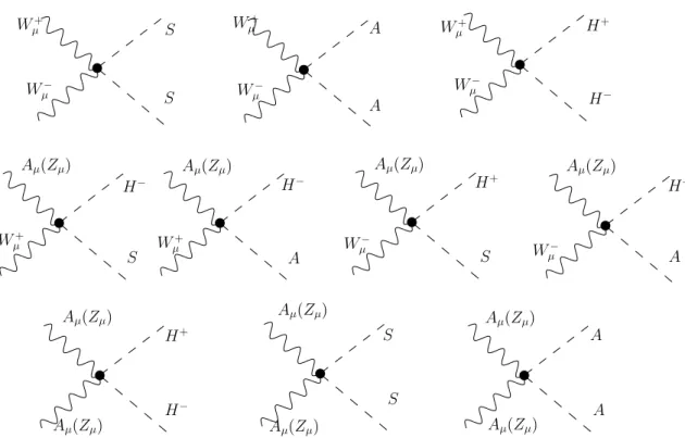
The quartic interactions between the Higgs doublet and the inert doublet are: Vq = ((λ3 + λ4)φ+φ−H+H−+ λ5 2 £ φ−H+φ−H++ h.c¤+ +λ3 · H+H−h 2+ χ2 2 + φ +φ−S2+ A2 2 ¸ + (λ4+ λ5 2 )(hS + χA)(φ −H++ h.c.) + + · ı(λ4− ıλ5 2 )φ +H−Ah + h.c ¸ + · ı(λ4+ ıλ5 2 )φ +H−Sχ + h.c. ¸ + (4.8) +1 4[(λ3+ λ4 + λ5)(hhSS + χχAA) + (λ3+ λ4− λ5)(χχSS + hhAA)] + +λ5SAhχ.
where χ is the neutral Goldstone boson and the other particles are those we introduced before. Those interactions are shown in figure (4.2).
20 CHAPTER 4. THE MODEL H− H+ H− H+ H+ H− φ− φ+ φ− φ+ φ− φ+ S S A A χ χ h h φ+ φ+ φ+ φ+ H− H− H− H− χ χ S A h S h A h h h h χ χ χ χ χ h S A A S S A A S S A
Figure 4.2: Vertexes given by the quartic couplings of the ID to the SM Higgs doublet.
4.2. INTERACTIONS 21
4.2.2
Interactions with Gauge Bosons
The inert doublet also interacts with Gauge Bosons because of the term
|DµH2|2in the free lagrangian. In terms of the mass eigenstates Wµ+, Wµ−, Zµ
and Aµ it is Dµ= ∂µ− ıg √ 2 ¡ W+ µ σ++ Wµ−σ− ¢ − ıg cosϑW Zµ ¡ T3− sin2ϑ WQ ¢ − ıeAµQ (4.9) where g = √2mW
v is the weak coupling constant (mW is the W mass and v
is the Higgs vev), sin2ϑ
W = 0.23 where ϑW is the weak mixing angle,σ± = σ1± ıσ2 with σ1 and σ2 the two non diagonal Pauli matrices, Q is the electric charge and T3 the third component of the weak isospin. Both Q and T3 are referred to the particle the Z,or the A, is interacting with.
Applying Dµto the inert doublet as it is parametrized in (4.3) and
squar-ing its modulus we find that its quartic interactions are:
|DµH2|2 ⊃ g2 · W+ µWµ− 2 µ S2+ A2 2 ¶ +W + µWµ− 2 H +H− ¸ + (4.10) +gg 0 4 (cosϑWAµ− sinϑWZµ) h√ 2S(W− µH++ Wµ+H−) + √ 2ıA¡W+ µH−− Wµ−H+ ¢i + +gg0 2 ¡ cos2ϑ WAµAµ− sin2ϑWZµZµ ¢· H+H−− 1 2S 2 −1 2A 2 ¸
where g0cosϑW = gsinϑ
W. The particles involved in those coupling are
the four particles belonging to the inert doublet: φ+, φ−, S, A plus the four
gauge bosons: W+
µ, Wµ−, Zµ and Aµ. The quartic interactions between the ID and the gauge bosons is shown in figure (4.3). The cubic interactions
between the inert doublet and the gauge bosons are:
|DµH2|2 ⊃ ıg 2(−2sinϑWAµ £¡ ∂µH− ¢ H+−¡∂ µH+ ¢ H−¤+ (4.11) + Zµ cosϑW ©
ı (∂µS) A − ı (∂µA) S +¡sin2ϑW − cos2ϑW¢ £¡∂µH−¢H+−¡∂µH+¢H−¤ª+ +S£¡∂µH− ¢ Wµ++¡∂µH+ ¢ Wµ−¤− ıA£¡∂µH− ¢ Wµ++¡∂µH+ ¢ Wµ−¤ + (∂µS)¡Wµ+H−+ Wµ−H+¢+ ı (∂µA)¡Wµ+H−+ Wµ−H+¢)
The derivative contributes to the vertex with a factor −ıkµ if the momentum
of the particle on which the derivative acts points into the diagram. For exam-ple the first line of (4.11) gives this contribution: −gsinϑW [pµ(H−) − pµ(H+)]
where pµ(H−) is the momentum of the H−and pµ(H+) is tho one of the H+.
22 CHAPTER 4. THE MODEL W+ µ W + µ W− µ W− µ W− µ W− µ S S A A H− H+ W− µ H− H− H+ S H− H+ S A A H+ S A A S W+ µ W + µ Wµ+ Aµ(Zµ) A µ(Zµ) Aµ(Zµ) Aµ(Zµ) Aµ(Zµ) Aµ(Zµ) Aµ(Zµ) Aµ(Zµ) Aµ(Zµ) A µ(Zµ)
Figure 4.3: Vertexes given by the quartic interaction of the ID with gauge bosons.
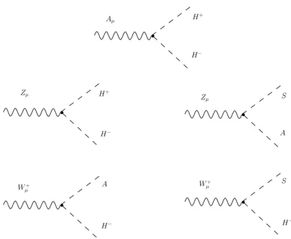
4.3. EWPT 23 Aµ Zµ Zµ W+ µ W+ µ H− H+ H− S A S A H− H− H+
Figure 4.4: Vertexes given by the cubic interaction of the ID with gauge bosons.
vertexes given from the cubic interactions between Id and gauge bosons are given in figure (4.4). It is important to stress that we have no interaction like
SSZ or AAZ. The only interaction of Z boson with the neutral components
of the inert doublet is ZAS. This will have important consequencies further on.
4.3
EWPT
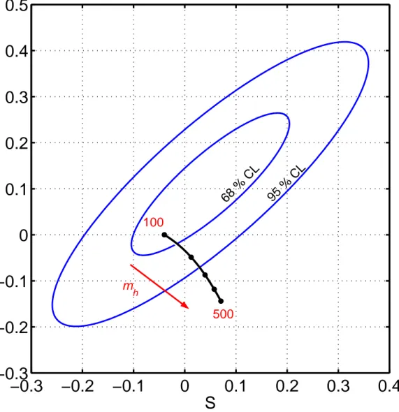
The extra doublet H2, for values of the couplings in (4.2) of order 1 can give significant contributions to the Electro Weak precision observables throught radiative corrections in particular to the T parameter (See figure (4.5)). This parameter, and the analog S, allow to characterize any new physical effect to the EW P O. In figure (4.6) we show the experimental determination of T and S and their prediction in the SM as a function of the Higgs mass.
An interesting fact is that the effects of the Inert Doublet to T can make a relatively heavy Higgs compatible with the EW P T , unlike the case of the Standard Model, where an Higgs heavier than about 160GeV is already excluded at 95%C.L.. The analysis of the EW P T in the model under ex-amination goes behind the scopes of this thesis. Making reference to [?] for
24 CHAPTER 4. THE MODEL χ χ A S φ+ φ+ φ+ φ+ S S A A H− H− φ− φ− φ− φ− H+ H+
Figure 4.5: Contribution of the inert doublet to T
such an analysis, here we only recall that a Higgs mass as heavy as heavy as 500GeV can indeed be made compatible with the precision tests, with coupling λ0s that remain perturbative up to a few T eV , provided that the
spectrum of the new particle satisfies the constraint
(mH − mS)(mH − mA) = M2 , M = 120 ± 30GeV (4.12)
where mS, mA, mH are the masses of the particles belonging to the inert
4.3. EWPT 25
−0.3
−0.2
−0.1
0
0.1
0.2
0.3
0.4
−0.3
−0.2
−0.1
0
0.1
0.2
0.3
0.4
0.5
S
T
68 % CL 95 % CL m h 100 500Chapter 5
Important Cross Sections
We will analize separately the cross sections of the processes that contribute to calculate the relic abundance of the L particle, and the cross section of the processes that can be used to detect the particle.
5.1
Annihilation cross section
As we said in the previous chapters,the lightest particle of the model is stable and the way its abundance is determined is throught annihilation into other
SM particles.
We have to consider separately two cases: when mL < mW and when mL > mW. In the first case L particles mostly coannihilate into fermions, while in the second case the main annihilation channel is into a W pair.
5.1.1
m
L< m
WIn this case L abundance decreases mainly throught p − wave coannihilation into fermions. The Feynmann diagram of the process is shown in figure (5.1.1). Obviusly we have to sum over all the cinematically allowed fermions. The time averaged cross section of this process is given by
σAS→f ¯fv® = bv2 (5.1) where b = µ g 2cosϑW ¶4 Σf(gV2 + gA2) 6π mN LmL [(mN L+ mL)2− m2Z] 2 (5.2)
The vector and axial coefficients gV and gA are summed over all fermions
except the top quarks,which are above threshold, so that Σf(gV2 +gA2) = 7.32.
28 CHAPTER 5. IMPORTANT CROSS SECTIONS
A
S
Z
f
¯
f
Figure 5.1: Coannihilations into fermions.
L W+ W− L L L L L W∗Z W−Z ZZ Z
Figure 5.2: Annihilation into gauge bosons. The second graphic is suppressed and does not contribute.
Evaluating the expression (5.2) for b, with mNL ∼ mL, it is
b = (25, 10)pb f or mL= (60, 80)GeV (5.3)
5.1.2
m
L> m
WIn this case L mainly annihilates into a gauge boson pair. When mLis fairly
bigger than mW we can consider gauge bosons massless and compute the
total cross section summing the cross section for annihilation into bosons with transverse polarization and the cross section for annihilation into longitudinal bosons. The processes contributing to annihilation into transverse gauge bosons are shown in figure (5.2), and their cross section is
σLL→⊥⊥vrel = g 4 64πm2 L µ 2 + 1 cos4θ W ¶ (5.4)
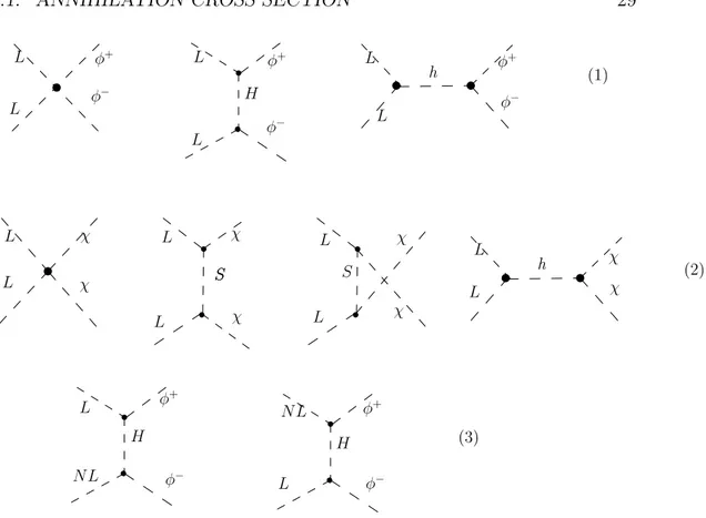
5.1. ANNIHILATION CROSS SECTION 29 L L φ+ φ− h L L φ+ φ− H L L φ+ φ− S L L χ χ S L L χ χ L L χ χ S H L N L φ+ φ− H L N L φ− φ+ h L χ χ L (1) (3) (2)
Figure 5.3: Annihilation into Goldstone bosons.
Evaluating this cross section for masses of L big enough to allow the massless
W approximation we find σLL→⊥⊥vrel ≈ 130pb µ 100GeV mL ¶2 (5.5)
Relatively more important can be the annihilations (and the coannihilations) into longitudinal gauge bosons, since they grow like the fourth power of the couplings λs in equation (4.2). The corresponding cross sections can be most effectively computed by considering the processes into the correspond-ing Goldstone bosons, χ and φ± for Z and W± respectively (figure (5.3)).
30 CHAPTER 5. IMPORTANT CROSS SECTIONS MSS,AA→χχ = λA,S+ λS,Am2h s − m2 h + 2λ2 5v2 Ã 1 t − m2 A,S + 1 u − m2 A,S ! MSS,AA→φ+φ− = λ3+ λS,Am 2 h s − m2 h +(λ4± λ5)2v2 2 µ 1 t − m2 H + 1 u − m2 H ¶ MSA→φ+φ− = ı(λ4± λ5) 2v2 2 µ 1 t − m2 H − 1 u − m2 H ¶ (5.6) For our purpose we can safely neglect the Mandelstam variables t and u as, by the time of f reeze out, they are negligible respect to the particle masses
mI.
With this approximation the coannihilation amplitude vanishes and the longitudinal cross section becomes
σLL→||||vrel ≥ 1 96πm2 L ½ |λ4| − |λ5| − (|λ4| + |λ5|)2v2 m2 H +4λ25v2 m2 N L ¾2 (5.7) Evaluating this longitudinal cross section of interest we find
σLL→||||vrel ≥ (10 − 50)pb f or mL= (100 − 800)GeV (5.8)
An important point is that this lower bound increases with mL, unlike
equa-tion (5.5) for the annihilaequa-tion into transverse gauge bosons. This is due to the increase of the couplings λi which more than compensate the m12
L factor.
This means that the sum of (5.5) and (5.13) is always above 50 pb in the whole range of mL
5.1.3
m
L∼ m
WWe have to be careful in analizing this range of masses, because, as we will see later, it is of fundamental importance in determining the relic abundance of the dark matter candidate.
As we are at threshold for annihilation into W bosons we cannot take W massless any more, nor we can consider the contribution to the total cross section due to annihilation into Z boson. The only diagram contributing to the cross section is the first in figure (5.2) and its contribution is
σLL→W W = g 4 128πvrm2L µ 3 + 4k 4 m4 W ¶ r 1 −4m 2 W s (5.9)
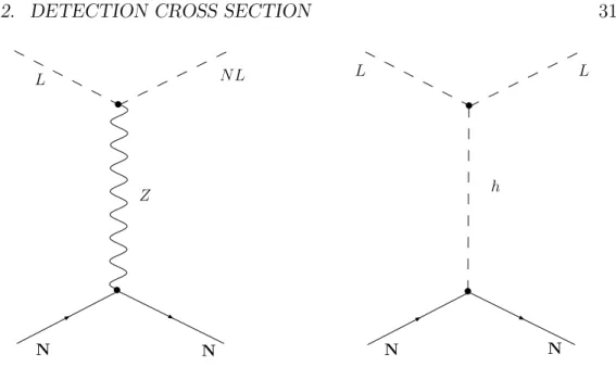
5.2. DETECTION CROSS SECTION 31 L Z N L N h L L N N N
Figure 5.4: Direct Detection through elastic scattering on nuclei.
5.2
Detection cross section
We can detect directly the L particle throught the detection of its scattering on nuclei by experiments dedicated to the search for dark matter. In principle there are two ways in which L can scatter off a nucleus, by a Z exchange or by a Higgs exchange ( figure (5.4)). Since L is highly non relativistic (β w 10−3), the inelastic process by Z exchange can only take place if NL is
very close in mass to L. In this case, neglecting ∆m at all, the cross section of this process, which does not depend on the spin of the nucleus but only on its total charge and mass, is
σZ(L → NL) = G2 Fm2r 2π £ N − (1 − 4sin2θ W)Z ¤2 (5.10) where mr = (mmLL+mmNN, is the reduced mass, N is the number of neutrons in
the nucleus and Z is the number of protons.
The CDMSII collaboration puts an upper bound [?] on the spin in-dipendent cross section per nucleon of dark matter on nuclei. This limit is
σ . 10−7pb for scattering on Germanium of a 60GeV W IMP . The cross
section in (5.10) is several orders of magnitude bigger than this bound. To make our particle compatible with the experimental limit we have to prevent it from interacting via the spin independent Z exchange. That is easily done setting the mass difference between L and NL bigger than the kinetic energy of the dark matter in our galaxy halo.
32 CHAPTER 5. IMPORTANT CROSS SECTIONS
is the elastic scattering on nuclei through an Higgs exchange. The cross section for this process again spin indipendent is
σh(LN → LN ) = 1 4πm 2 r µ λL mLm2h ¶2 f2m2N (5.11)
where f v 0.3 is the usual nucleonic matrix element:
hN |Σmqq ¯q|N i = f mN hN |N i (5.12)
Evaluating numerically this cross section for scattering from a proton we obtain: σh(Lp → Lp) ≈ 2 × 10⁻⁹pb µ λL 0.5 ¶2µ 70GeV mL ¶2µ 500GeV mh ¶4 (5.13) . The largest uncertainty in this extimation comes from the uncertainty on
λL. If we take λL = 0.5 the previous cross section is of order 10−9pb that is
below the bound quoted above for any Higgs mass above about 200GeV but could be within reach of planned experiments.
Another allowed process that can contribute to direct detection is the scattering on nuclei with the exchange of two gauge bosons at one loop. This process gives an effective coupling similar to the tree-level h exchange. Always neglecting the mass difference ∆m the cross section for this process can be estimate as σ(LN → LN ) ' m 2 r 4π · (g/2cW)4 16π2m3 Z ¸2 f2m2 N (5.14)
, which is independent of mL. For larger splittings this cross section acquires
a dependance on mL as the factor m3Z in the amplitude should be replaced
by mLm2Z
The cross section for direct detection in case mL > mW is suppressed
from the m−2L factor in σh. Moreover in this case the relic density is much
smaller than the previous case, as we will see in the next chapter. So the possibilities to see our particle if it is in this mass range is very reduced.
Chapter 6
Relic Abundances
In the previous chapter we have studied the cross section for the relevant processes that occur at decoupling of L particles. From these cross sections we now compute the relic abundance of the L particles in the various mass ranges. We look to see if there is a mass range in which our particle has a relic abundance similar to the dark matter relic abundance observed from experiments.
6.1
m
L. m
WWe have seen in the previous chapter that, in this range of L masses, there are two different processes that mainly contribute to modify the relic abundance of L particles. When mL< mW strictly, we have only the coannihilation of L and NL into fermions. When mL v mW the annihilation into Ws becomes
important in the calculation of relic abundance of L particles.
We will compute separately the relic abundance of L particles for each of these two cases and then we will put them together.
6.1.1
m
L< m
WIn case mL< mW the main reaction that decreases the number density of L
particles is their coannihilation with NL particles into a fermion-antifermion pair. To find the relic density in this case we have to apply the formalism developed for the first special case of chapter 3.
In our case there is only one cross section that contributes to σef f (3.3)
and it is the coannihilation cross section in (5.2):
σef f = 2 g2 ef f b µ mN L mL ¶3/2 exp µ −xmN L− mL mL ¶ (6.1) 33
34 CHAPTER 6. RELIC ABUNDANCES
The effective number of degrees of freedom for our problem is
gef f = 1(mN L
mL
)32exp(−xmNL mL
) (6.2)
As we said in chapter 5 this is a p − wave process. This greatly simplifies the annihilation integral (3.8). Inserting everything into the expression for Ωh2 in (2.14) we find that it depends only on mN L and mL as we expected.
6.1.2
m
Lv m
WSince in the thermal plasma before freeze out there is some thermal energy that could lower the threshold for L annihilating into W , we can apply in this case the formalism developed for the second special case of chapter 3.
The process involved in this case is a s − wave annihilation so we can derive the thermal averaged cross section directly from the formula found in (3.12). Coannihilation into fermions is still present in this range of masses but for mL> 70GeV its cross section is very suppressed with respect to the
cross section for annihilation into W s
6.1.3
m
L. m
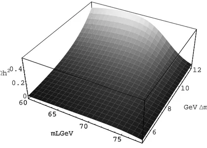
WPutting together the contribution to the relic abundance of L particles we derived in the previous sections we have found the plot in figure (6.1). The plot shows how Ωh2 varies as a function of m
L and ∆m
The plot in figure (6.2) is easierto analyze as it shows sections of the plot (6.1) with Ωh2 = cost. A brief analysis of the plot (6.2) evidences some features that we could have guessed even without seeing the plot.
The first of these features is that, for fixed mL, the bigger is the mass
difference, the bigger is the relic abundance of L particles. This is because, since the next to lightest particle is Boltzmann distributed, the bigger is its mass, the smaller is its density, which is exponentially suppressed with ∆m. But the smaller is the density of NL particles, the smaller is their coannihi-lation rate with L particles. This leads to an increase in the abundance of L particles when the mass of the NL particles increases.
Another feature of the plot in figure (6.2) is that the curves representing Ωh2 = cost grow for m
Lv 72GeV . This is easily explained with annihilations
into Ws that increase the effective cross section. A bigger mass difference is then needed to obtain the same relic abundance we had when the effective cross section was only due to coannihilations into fermions.
Given the experimental limits on dark matter abundance that are, as we said before, Ωh2 = 0.09 ÷ 0.12. We can see that for masses bigger than about
6.1. ML. MW 35 60 65 70 75 mLGeV 6 8 10 12 GeVDm 0 0.2 0.4 Wh2 60 65 70 75 mLGeV Figure 6.1: Ωh2 as a function of m L and ∆m
Figure 6.2: Ωh2 = 0.07 (black), Ωh2 = 0.1 (blue),Ωh2 = 1.2 (green),Ωh2 = 0.15 (red) in the plane mL, ∆m
36 CHAPTER 6. RELIC ABUNDANCES
76GeV there is no mass splitting that makes the relic abundance compatible with experimental limits
From plot (??) we can draw an important conclusion: for mL . 76GeV
there is a mass splitting ∆m in the range (7 ÷ 12GeV ) that gives a value for the relic abundance of L particles compatible with the experimentally measured one.
6.2
m
L> m
WWhen mL> mW we can neglect the W masses and we can apply the standard
formulas found in chapter 2. It is very simple to see that in this mass range there is no way to obtain a relic abundance compatible with the experimental one. The annihilation cross section into a pair of gauge bosons is simply too big to leave a sufficient abundance of L particles, so this mass region is excluded if we want our particle to solve the dark matter problem.
Chapter 7
Summary and Conclusions
7.1
Collider signals
Before concluding we would like to make few comments on possible collider signals for values of the L and NL masses that makes L a possible candidate to explain the dark matter. In fact, if mL≈ 70GeV and ∆m is small, S and A pairs could have beenproduced at LEP 2. The production cross section for
∆m ¿ mL is σ(e+e− → S A) = µ g 2cW ¶2µ 1 2 − 2s 2 W + 4s4W ¶ 1 48πs [1 − 4m2 L/s]3/2 [1 − m2 Z/s]2 (7.1) which, for √s = 200GeV , gives σ(e+e− → S A) ∼ 0.2pb. The heavier state NL decays into the lighter plus a virtual Z, giving soft jets plus missing
energy. This signal has in fact been studied at LEP 2. However, for ∆m . 10GeV the production cross section of 0.2pb is below the LEP 2 limits. At the LHC our particles will be pair produced both through a W or a Z. A detailed study of the background to various decay channels is required to assess their detectability.
Let us finally briefly comment on the Higgs decay into a pair of scalars that compose the inert doublet.
h → SS h → AA h → H+H−
Their contribution to the Higgs width is ∆Γ = v 2 16πmh " λ2S µ 1 −4m 2 S m2 h ¶1 2 + λ2A µ 1 −4m 2 A m2 h ¶1 2 + 2λ23 µ 1 − 4m 2 H m2 h ¶1 2 # (7.2) In figure () I give an isoplot of ∆Γ
38 CHAPTER 7. SUMMARY AND CONCLUSIONS
7.2
Conclusions
In this thesis we have studied a simple model where the DM may be explained by a weakly interacting neutral scalar of mass below the mass of the W .
The model consists of a scalar doublet added to SM. The doublet is pro-tected from interacting with fermions by a conserved Z2 symmetry, therefore we referred to it as Inert Doublet. However the inert doublet is coupled to the Higgs boson and to the gauge bosons. Unlike the Higgs doublet, the inert doublet does not acquire vev. The mass spectrum of the Inert Dou-ble consists of three particles, two neutrals, which we called S and A, and one charged, H. The lightest particle of the doublet, which we called L and could be either S and A depending on the values of the coupling constant in the scalar potential (4.2) should be neutral to be consistent with EW P T , so also the next lightest particle (NL) should. The lightest particle of the Inert Doublet is thus neutral, massive and stable, that makes it a DM candidate.
To assess the relic abundance we have studied the annihilation and coan-nihilation cross sections. For mL> mW the relic abundance of L particles is
too small, so that it cannot account for all the experimentally observed DM. For mL < mW we have also too little relic abundance of L particles due to
the fact that the Z exchange cross section is still too big. However Z ex-change is only present for coannihilations, so that the correct abundance can be obtained by a suitable correlation between mL and mN L. This correlation
becomes of fundamental importance when speaking about the possibility of detecting the particle: the cross section for Z mediated scattering on nucleus, in which has one between L and NL is the scattering particle and the other is the scattered particle, is several orders of magnitude bigger than the present experimental limits. Since this scattering has never been observed we have to set the parameters to suppress this type of interaction. This is achieved setting the mass difference between L and NL bigger than the kinetic energy of our galaxy halo.
The cross section for its detection through scattering on nuclei via Higgs exchange in certain ranges of masses could be within the reach of planned experiments.
We have not discussed the possibility of detecting indirectly the lightest particle of the inert doublet, through the detection of secondary particles coming from dark matter annihilation in the halo of the galaxy. The inter-ested reader can find an extensive discussion of the photon detection in [?].