A multi-instrumental approach to the study of equatorial ionosphere over South America

Alma Mater Studiorum – Università di Bologna

DOTTORATO DI RICERCA IN

GEOFISICA

Ciclo XXVII

Settore Concorsuale di afferenza: 04/A4 - GEOFISICA

Settore Scientifico disciplinare: GEO/10– GEOFISICA DELLA TERRA SOLIDA

TITOLO TESI

A multi-instrumental approach to the study of equatorial

ionosphere over South America

Presentata da:

Claudio Cesaroni

Coordinatore Dottorato

Relatore

Prof. Michele Dragoni

Dott. Carlo Scotto

… To whom is already here

and to whom is about to be.

Introduction 5

1. The Equatorial Ionosphere 8

1.1 The ionosphere 8

1.2 Ionospheric vertical structure 9

1.3 Geographical and seasonal variations in the ionosphere 13

1.4 Electrodynamics of the Equatorial ionosphere 16

1.4.1 Equatorial electrojet 17

1.4.2 Vertical drift and Equatorial ionization anomaly (EIA) 18

1.4.3 Rayleigh-Taylor instability and plasma bubbles 18

1.5 References 21

2. Ground based measurements and models for ionospheric studies 22

2.1 GNSS and ionospheric effects on satellite signals 22

2.1.1 Ionospheric refractive index and Total electron content 24

2.1.2 L-band scintillations 25

2.2 HF radar for ionospheric vertical soundings 27

2.2.1 The virtual height of an ionospheric layer 28

2.2.2 Vertical ionograms 30

2.2.3 Autoscala: software for automatic interpretation of the vertical ionograms 31

2.2.4 Adaptive Ionospheric Profiler (AIP) 31

2.3 NeQuick model for ionospheric electron content 35

2.3.1 Bottomside ionosphere modelling 35

2.3.2 Topside ionosphere modelling 36

2.4 References 38

3. TEC gradients and scintillation climatology over Brazil 39

3.1 Data and methods 41

3.1.1 URTKN and CIGALA networks 41

3.1.2 TEC calibration technique 44

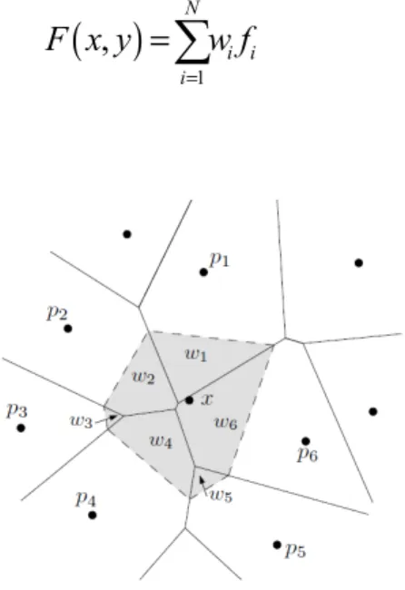
3.1.3 Calibrated TEC interpolation and spatial gradients. 46

3.1.4 Ground based scintillation climatology (GBSC) 48

3.2 Results 49

3.2.1 Climatological analysis 49

3.2.2 Case studies 57

3.3 Validation of the results in the “position domain” 61

3.3.1 Data description 61

3.3.2 Long-baseline RTK algorithm 62

3.3.3 Performance of IGS and CTM maps 64

3.5 Conclusions 69

3.6 References 70

4 Zonal velocity of the ionospheric irregularities 74

4.1 Measurement technique 74

4.2 Algorithm description 76

4.2.1 Scintillation pattern velocity 77

4.2.2 Satellites position and velocity 79

4.3 Micro Test Area 81

4.3.1 Description 81

4.3.2 Data availability 83

4.4 Results 85

4.4.1 Comparison with indipendent measurements 85

4.4.2 Zonal velocity and scintillations occurrence 87

4.5 Conclusions 89

4.6 References 90

5. NeQuick model validation over Tucuman (Argentina) 91

5.1 Data and method 91

5.2 Results 95

5.2.1 Quality evaluation for f0F2 given by Autoscala 95

5.2.2 Comparison between GNSS TEC and NeQuick TEC over Tucuman 96

5.3 Conclusions 100

5

Introduction

Since the end of the nineteenth century, when Guglielmo Marconi realized his experiment for the transmission of radio waves across the Atlantic (between Poldhu in Cornwall and Clifden in Co. Galway), the existence of an ionized layer in the upper atmosphere was argued. Only in 1926, Scottish physicist Robert Watson-Watt introduces the term ionosphere and, one year later, the physicist Edward V. Appleton confirmed the existence of the ionosphere with his experiment of phase interference patterns. As the Breit and Tuve developed the first ionosonde, different kind of experiments and instruments was developed in order to measure the height and the density of the ionized layers of the upper atmosphere mostly because the importance of the radio transmission for military purposes increased. In the second half of the twentieth century, with the increase of technological and scientific interest in the propagation of electromagnetic waves through the atmosphere, also satellite missions have been realized to study the physics governing the morphology and the dynamics of the ionosphere. Some example are the missions Alouette 1 and 2 launched in 1962 and 1965 respectively and ISIS satellites launched in 1969 and 1971 respectively. All these missions was devoted mainly on the study of the ionospheric electron density distribution during quiet and disturbed helio-geophysics conditions. In fact, It was well known since the first studies of the terrestrial ionosphere that the behaviour of the ion and electron in the upper atmosphere is strictly governing by the solar activity and influenced by the geomagnetic field. In the meanwhile, US Navy starts to develop a satellite mission named

Transit with the aim to furnish a positioning service to the ship during navigation in all weather conditions.

First of the six Transit satellites reached its orbit in 1960 and since 1967 the first satellite positioning service was made available. Tacking advantage from the experience of Transit US Department of Defence started to develop a new satellite fleet and in 1994 the Global Positioning System (GPS) services was made available. These satellites, as the Transit ones, transmit on two different frequencies to correct, at least partially, the error induced by the ionosphere. From this, it is clear that, from another point of view, GPS signals can be used to infer information about the ionized upper atmosphere. The global coverage of the GPS and decreasing costs related to the receiver installation and maintenance, make the GPS one of the most used instruments for the investigation of the ionosphere. After the introduction of the GPS some other countries have been developed their own system to allow satellite based positioning such as Russia (GLONASS), China (BiDou) and finally the European community (GALILEO). All these systems is generally named GNSS (Global Navigation Satellite System)

The interaction between the ionosphere and the geomagnetic field lead to some particular features of the ionosphere especially in the low and high latitude regions. In particular, in the region near the geomagnetic equator, the coupling between electric field, generated by thermospheric neutral wind, and the horizontal magnetic field creates a vertical movement of the ionospheric plasma. This vertical drift is the main responsible for the “noise” (known as scintillation) experienced by GNSS signals crossing the low latitude

6 ionosphere. The influences of the scintillations on the signal can lead to a degradation of the positioning performance and even to a complete loss of the signal tracking by the receiver.

In the framework of the FP7 programme, CALIBRA (Countering GNSS high Accuracy applications LImitation due to ionospheric disturbance in BRAzil) project was running until February 2015 with the aim to develop countermeasures against the ionospheric disturbances to the high precision GNSS applications in Brazil. A specific working package, leaded by INGV, was dedicated to the ionospheric assessment and, in particular, to the relationship between TEC (Total Electron Content), its spatial gradients and the GNSS scintillation phenomenon occurrence.

This thesis is part of the work performed during this project by the author in strict collaboration with the partners of the project and, in particular, with the INGV people involved in CALIBRA and the Nottingham Geospatial Institute. In the first chapter of this dissertation an overview on the morphology of the ionosphere and its regular variation is given. Particular emphasis is posed on the topics related to the equatorial ionosphere electrodynamics that drive the phenomena described in the next chapters. In chapter 2 an overview of the instruments and technique used to perform all the analysis presented in this thesis is given. Section 2.1 treat the use of GNSS receivers to study the morphology and dynamics of the equatorial ionosphere over Brazil in terms of TEC, scintillations and velocity of the ionospheric irregularities. Section 2.2 is devote to the description of the ground based HF radar (ionosonde), an instrument used to retrieve electron density vertical profile by using an automatic interpretation software developed at INGV (Autoscala, described in section 2.2.3). Last section of chapter 2 (2.3) describe an electron density model, the NeQuick, able to give TEC climatological estimation starting from some fundamental ionospheric parameters (M(3000)F2 and foF2). This model is the one adopted by ESA to give ionospheric correction to the users of

the new European GNSS constellation GALILEO. Last part of this thesis is devoted to the validation of such model used to retrieve TEC at low latitude regions.

The core of this thesis is given in chapter 3,4 and 5. In the first one the description of the analysis of TEC, its spatial gradients and amplitude scintillation is given in order to establish a relationship between the morphology of the distribution of the electron and the scintillation experienced by GNSS signal. Different original and known technique is applied in order to reach the objectives. Results are given in section 3.2 and summarized in section 3.3. Main conclusions are reported in section 3.4 highlighting the importance of the meridional TEC gradients in the occurrence of the scintillations and confirming the high occurrence of the strongest scintillations in the post sunset hours during spring and summer. Validation of the results by means of their use in the precise positioning algorithms applied in Brazil is given in section 3.3. This section reports the work performed in collaboration with Nottingham Geospatial Institute and described in detail in a paper submitted to Journal of Geodesy, at present, under review. This work is also part of a project funded by ESA

7 and in which the author is involved as tasks leader. This project highlights the importance of the results reached in this thesis also from the technological point of view in the field of the satellite navigation and high precision GNSS applications at low latitude regions.

Chapter 4 is devoted to the analysis of high sampling rate GNSS receivers deployed in Brazil. In particular, two close receivers (about 300 meters far each other) give the opportunity to study the zonal velocity of the small scale ionospheric irregularities by means of an original algorithm (section 4.2) developed by the author starting from the equations and discussions presented by Ledvina et al., 2004. Important results about the correlation between this velocity and amplitude scintillation occurrence is given in section 4.4 together with the comparison between the velocity inferred by this technique and by means of other independent instruments such as Incoherent scatter radar and ionosonde.

Finally, in chapter 5 a validation of the NeQuick model at low latitude region is described. By means of GNSS- derived TEC values and ionosonde derived parameters (M(3000)F2 and foF2) and slightly modifying the

source-code of the model, is shown that the model can improve its performance if it ingests parameter measured by an ionosonde instead of modelled one (section 5.2). In addition, a proper selection of the ionosonde data input can be applied to further improve the performance of the model in terms of TEC estimation. This algorithm to automatically evaluate the goodness of the ionosonde derived parameters was developed in the framework of this thesis and it is published in a paper on Advances in Space Research (Cesaroni et al., 2013).

8

1.

The Equatorial Ionosphere

This initial chapter provides an outline of some fundamental concepts regarding the formation of the ionosphere and its cyclical variations. A theoretical basis is established in order to better understanding the research described in the subsequent chapters. Certain important phenomenon that occur at low latitudes and in the equatorial ionosphere are specifically analysed as an introduction to the results presented in this thesis.

1.1 The

ionosphere

The region above 80 km is generally classified as the "upper atmosphere". Due to the low density of neutral particles at this altitude, the free electrons created from the ionization process can survive for a significant time before recombination with ions. The ionization process involves the stripping or addition of one or more electrons from atoms or molecules resulting in positively or negatively charged particles. In the upper atmosphere there is a marked prevalence of positively charged ions generated by loss of an electron rather than negatively charged ions with an extra electron. Ionization in this context occurs when electrons are dislodged from their host ions either by high-energy solar photons (mainly UV and X-rays) or energetic particles precipitating into the atmosphere and colliding with atmospheric gasses. The traditional atomic model (referred to as the "Bohr model" in acknowledgement of this scientist's role in its development) includes one or more electrons orbiting a nucleus of sub-atomic particles called protons and neutrons. Protons exhibit equal but opposite positive and negative charges, respectively. Opposite charges are attracted to each other with what is called the electrostatic or Coulomb force, while matching charges (negative/negative or positive/positive) repel each other. The vast majority of atoms and molecules in the Earth’s lower atmosphere have the same number of protons and electrons in each atom making them neutral,. However, in the upper atmosphere there are appreciable numbers of charged particles (ions and electrons). The number of free ions and electrons peaks at altitudes around 300 km forming a region known as the "ionosphere". The vertical structure of this region is shown schematically in Figure 1. The ionosphere is generated primarily by solar electromagnetic radiation in a process called photoionization, with the consequence that the ionosphere is most dense during local daylight hours. The ionosphere does not entirely disappear at night because the necessary recombination time for the ions and electrons (the average time required for all the ions and electrons to unite to form neutral particles) is long enough for the layer to persist overnight. The recombination rate is determined by background density and is consequently high at low altitudes (where density is high), and decreasing with altitude as the density falls. The degree of ionization at any given point is a balance between the rate of production of ions (photoionization), and the rate of loss of ions (recombination).

9

1.2 Ionospheric

vertical

structure

There is a tendency for the terrestrial ionosphere to separate into layers at all latitudes, even though different processes are seen to dominate at different latitudes. The D, E, F1, and F2 layers are, however, only distinct at mid-latitudes in the diurnal ionosphere. The various layers generally exhibit a maximum density at a given altitude, with decreasing density above and below the maximum value. Historically, the E layer was discovered first, followed by the F and D layers. The E and F layers are usually defined as shown in Figure 1 using critical frequencies (foE, foF , foF2), peak heights (hmE, hmF1, hmF2), and half-thicknesses (ymE, ymF1, ymF2). The critical frequency is proportional to

n

a layer. Any higher frequency electromagnetic waves transmitted upwards towards the layer will pass through it to higher altitudes. A peak density (NmE, NmF1, NmF2) and peak height (altitude of maximum

density) are associated with each critical frequency. It is also common to define a half thickness for each specific layer, established from the best fit of a parabola to the electron density profile, within a range of altitude centred on the maximum density. All layers appear during the day, but the F1 layer decays during the night, and the E and F2 layers can be separated by the formation of a distinct E–F valley .

Figure 1. Electron density profiles for daytime (labeled f0F1) and nighttime ionosphere (labeled E-F valley). In the figure critical frequencies, peak heights and half-thicknesses for the different layers are also shown. From “Ionospheres

Physics, plasma physics and chemistry, Schung and Nagy

Molecular ions (NO+_{, O}

2+ , N2+ ) are dominant in the E region with short enough chemical time constants so

that plasma transport processes can be ignored. Photochemistry prevails in this context. Notwithstanding the large number of minor ion species in the E region, just a few photochemical processes are sufficient to

10 provide a good approximate description of the main ions. Since photochemistry is more important here than transport processes, the ion continuity equation for species s can be reduced to:

s

s s

dn

P L

dt

= −

where P_s is the production rate and L_s is the loss rate.

A few simplifying assumptions make it possible to establish an analytical expression for electron density in an ionosphere dominated by photochemical reactions. First, one of the molecular ions is assumed to be dominant, implying equality of ion and electron densities. During most daylight hours the time derivative term in the continuity equation is negligible, and the equation can be reduced to:

2

e d e

P k n

₌

where k_d is the ion–electron recombination rate. Next, it is assumed that the Chapman production function is suitable to describe an ionization rate as a function of altitude, z, and solar zenith angle, χ, giving the derivation:

(z, ) I

(z)e

P

_χ

_ησ

n

=

(z) n

n

₌

e

and where n(z) is the neutral density , H is the neutral scale height, σ is the absorption cross section, I_∞ is the flux of radiation incident on the top of the atmosphere, η is the ionization efficiency, τ is the optical depth, and z₀ is a reference altitude. If the reference altitude is chosen to be the level of unit optical depth (τ = 1) for overhead sun (χ = 0◦), the production rate at z₀ becomes

1 0

I

e

P

_ησ

n

=

The Chapman production function can thus be written as:

0

0

(z, )

exp 1

exp

sec

c c

z

z

z z

P

P

H

H

χ

=





−

−

−





_

−





_

χ









11 Finally, substitution of the Chapman production function in the continuity equation gives an expression for the Chapman layer:

1/2

0

1

(z, )

exp

1

exp

sec

2

P

z z

z

z

n

k

H

H

χ

=

















−

−

−





_

−





_

χ





















It should be noted that near the layer peak (z ≈ z0) the exponentials can be expanded into a Taylor series, and

the expression for the electron density can be reduced to

(

)

for overhead sun (χ = 0◦). The electron density profile is thus parabolic near the layer peak, explaining why half-thicknesses are defined in relation to a parabolic shape.

Generally the F region is divided into three subregions. Photochemistry is dominant in the lowest region labelled F1. The region of transition from dominance of photochemistry to diffusion is labelled F2, and the upper F region dominated by diffusion is called the ionosphere topside. The photochemistry in the F1 region is simplified because a single ion (O+) is dominant. Photoionization of neutral atomic oxygen and losses in reactions with N2 and O2 are the most important reactions. Transport processes become increasingly

important in the F2 and upper F regions. These include electrodynamic drifts across B, and ambipolar diffusion and wind-induced drifts along B. The magnetic field is essentially straight and uniform at F region altitudes in the latitude ionosphere, but also inclined to the horizontal at an angle I. However, the mid-latitude ionosphere is horizontally stratified resulting in vertically aligned density and temperature gradients (and gravity). The inclination of the B field limits the possibility for diffusion and constrains the charged particles to diffuse along B as a result of the low collision-to-cyclotron frequency ratios. The wind-induced and electrodynamic plasma drifts are also affected by the inclined B field. If ua|| is the ambipolar diffusion

component of ion velocity along B, then for a vertical force F (g, dT/dz, dn/dz), difussion is driven by the component of F along B, so that ua|| ∝F sin I. The vertical component of the ambipolar diffusion velocity,

inserted into the continuity equation, is uaz = ua|| sin I, so that uaz ∝F sin2 I . A meridional neutral wind and a

zonal electric field both induce vertical plasma drift . With an equatorward neutral wind (un), the induced

plasma drift along B is un cos I while the vertical component of plasma velocity is un sin I cos I. Finally, an

eastward electric field produces electrodynamic drift with a vertical component equal to (E/B) cos I. Taking all three plasma drifts into account, the ion diffusion equation can be expressed as

2

1

1

1

cos

sin cos

sin

iz n a i p p

T

n

E

u

I u

I

I

ID

B

n

z

T

z

H



_∂

_∂



=

+

−



_

+

+



_

∂

∂





12 where

H

=

2

kT

/

( )

m g

The basic shape of the F layer is not affected by neutral winds and electric fields and so their influence can be temporarily ignored. Diffusion is not significant in the daytime F1 region at mid-latitudes and time variations are slow. The O+ (or electron) density can thus be calculated by simply equating the production and loss terms (see Eq.(1.1)). The O+ density increases exponentially with altitude when chemical equilibrium is prevalent (Figure 2).

Figure 2. Chemical and diffusive equilibrium profiles and associated mid-latitude F region O+ _{profile. From “Ionospheres} Physics, plasma physics and chemistry, Schung and Nagy

This is a result of the O+ photoionization rate being directly proportional to the atomic oxygen density, which decreases with altitude exponentially, although less rapidly than the decline in N2 and O2 densities. The

overall consequence is an exponential decrease in O+ density with altitude. In the upper F region, diffusion is instead dominant, and generally the O+ density presents a diffusive equilibrium profile (Figure 2) generated by setting the parenthesis in the equation (1.10) to zero. O+ density therefore decreases exponentially with altitude at a rate dependent on both the plasma temperature gradient and scale height. The peak density of the F region occurs at the altitude where the prevalence of diffusion and chemical processes are balanced, with equal chemical and diffusion time constants. As already noted, at F region altitudes the charged particles

13 are constrained to move along B. A neutral wind in a poleward direction thus induces a downward drift of plasma, while a wind towards the equator induces an upward drift of plasma. Similarly, an electric field oriented towards the west induces a downward plasma drift, and an electric field towards the east induces an upward plasma drift. An upward plasma drift shifts the F layer to higher altitudes where the O+ loss rate is lower, causing an increase in both NmF2 and hmF2. The opposite occurs when there is a downward plasma

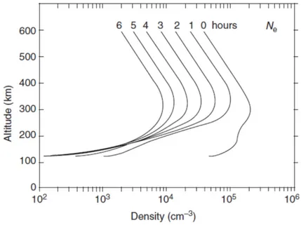
drift. There is no photoionization at night and the ionosphere decays. Figure 3 illustrated this decay in an idealized situation, ignoring nocturnal sources of ionization.

Figure 3 shows ionospheric decay in the absence of ionization sources, although this situation is not representative of true nocturnal conditions because different sources of ionization other than direct photoionization do exist at night. The nocturnal E region is maintained by production from starlight and resonantly scattered solar radiation (H Lyman α and β). The nocturnal F region is maintained to some extent by a downward flow of ionization from the upper plasmasphere.

Figure 3. Nocturnal decay of the electron density in the F layer after setting photoionization rate to zero. From “Ionospheres Physics, plasma physics and chemistry, Schung and Nagy

1.3

Geographical and seasonal variations in the ionosphere

There are marked variations in the Earth's ionosphere with changing seasons, latitude, longitude, altitude, universal time, solar cycle, and magnetic activity. Variations are exhibited in all ionospheric parameters including electron density, ion and electron temperatures, and ionospheric composition and dynamics. This is largely a consequence of the coupling of the ionosphere with other components of the solar-terrestrial

14 system: sun, interplanetary medium, magnetosphere, thermosphere, mesosphere, and to a limited extent also the troposphere and stratosphere . Variations fall into two general categories. The first are reasonably regular, within cycles or quasi-cycles that can be forecast with reasonable accuracy within "quiet" ionospheric conditions. The second are irregular, deriving mostly from sporadic behaviour of the sun and geomagnetic field, difficult to forecast, and representing "disturbed" ionospheric conditions.

Variations in ionospheric electron density caused by temporal cycles can be classified as: diurnal, day-to-day, seasonal, and solar cycles. The effects of the geomagnetic field on the ionosphere also produce regular geographical variations. Overall, five main variations in ionospheric electron density can be defined and need to be taken into account:

1. diurnal variation during daylight hours due mainly to the changing solar zenith angle; 2. seasonal variation during the year;

3. geographic and geomagnetic location; 4. long term solar cycles and disturbances; 5. height variations and the different layers.

These variations have all been experimentally established in worldwide ionospheric observations over recent decades. Routine ionospheric monitoring can be used to establish diurnal, seasonal, solar cycle, and height variations. Figure 4 and Figure 5 illustrate these four variables at a typical mid-latitude station, respectively during solar maximum and minimum, as indicated by the T parameter values.

Figure 4. Daily variation of the critical frequencies of the ionospheric layers (E, F1, F2) during the solar maximum in 1958 registered at Camberra station (mid-latitude). Left panel shows measurements carried out in June and right panel shows

15

Figure 5. Daily variation of the critical frequencies of the ionospheric layers (E, F1, F2) during the solar minimum in 1964 registered at Camberra station (mid-latitude). Left panel shows measurements carried out in June and right panel shows

January measurements.

Figure 4 and Figure 5 clearly show that the critical frequencies of the ionospheric layers are higher during a solar maximum than during a solar minimum. Figure 4 also shows an example of the mid-latitude seasonal anomaly, which is the seemingly unlikely fact that foF2 is higher in winter than in summer, despite the larger

solar zenith angle.

Figure 6 also illustrates how the F2 layer critical frequency, foF2, varies at 00 UT in June around the world,

under both high and low solar activity. Variations by location were quantified in an international campaign of measurements and data exchange. The relatively simple structure of the E and Fl layers, with foE and foF1

contours closely matching the solar zenith angle contours, is seen to be no longer valid, although a clear dependence on zenith angle is observed around sunrise. foF2 is also seen to vary by latitude, which is not the

case for foFE and foF1. In Figure 6, foF2 is seen to exhibit two afternoon peaks either side of the equator, a

16

Figure 6. Geographical variation of the critical frequency of the layer F2 during summer for solar minimum (top panel) and maximum (bottom panel).

1.4

Electrodynamics of the Equatorial ionosphere

Since the 1960s, routine ionospheric monitoring has highlighted that the equatorial ionosphere behaves very differently in certain respects from the ionosphere elsewhere. These differences were found to be caused not by the geographic equator but rather by the dip (or magnetic) equator. The dip equator is defined by the locus of points at which the dip angle of the magnetic field is zero, coinciding with the geographic equator only in two points. The orientation of the dip equator relative to the geographic equator is shown in Figure 7, where it clearly emerges how the main variation between the two is over South-America, which is the region considered in the present thesis.

17

Figure 7. Position of the dip equator (black tick line) with respect to the geographic equator (black thin line).

1.4.1 Equatorial electrojet

At high latitudes the electrodynamics are controlled by an interaction between solar wind and magnetosphere. At the equator the electrodynamics are instead driven by thermospheric winds, which generate the equatorial electrojet and are strongly influenced by the magnetic configuration in the equatorial region. The magnetic field in this region is oriented horizontally from south to north with the field aligned direction lying along the meridian plane. At heights over about 100 km the conductivity parallel to the magnetic field is so strong that the magnetic field lines are almost equipotential with the result that only the zonal (east-west) and vertical directions contribute to the electrodynamics. Below 100 km the conductivity is so weak that this lower ionospheric region makes no significant contributions to the overall dynamics. Thermospheric winds are oriented towards the east during the day and generate an eastward electric field EP. A vertical Hall current develops as a consequence of this electric field,, mainly due to the electrons, flowing

downwards during the day. Subsequently, vertical charge separation occurs in the ionosphere and a vertical electric field EH develops, constraining the ions in a vertical motion. This acts to reduce the vertical Hall

current until it becomes strong enough to block the Hall current completely. Averaging a magnetic field line, by integrating the entire length of the line (characterized by the curvilinear abscissas) gives:

P P S S

E



_σ



_σ

The polarization electric field EH is clearly very influential in the lower ionosphere given that integrated σ_S is

much lower than integrated_σP in this zone. This electric field commonly generates a strong eastward Hall current, known as the equatorial electrojet, further enhancing the zonal direction current JP. This is how the

atmosphere and magnetosphere are coupled. However, Pedersen conductivity rapidly decreases with altitude, along with EH, so that the polarization field EH is only strong over a limited range of latitude, limiting

18

1.4.2 Vertical drift and Equatorial ionization anomaly (EIA)

At altitudes above 100 km, the magnetic field traps ions and electrons. Analogous to the effect at high latitudes, a vertical convectional plasma drift is generated by the Pedersen electric field (caused by the neutral wind), so that with an eastward electric field, the ionosphere is raised higher. At high altitudes this vertical transport gives way to diffusion along the magnetic field lines as a consequence of the influence of gravity. Overall, ionospheric plasma exhibits a fountain-like movement in the equatorial region, known as the equatorial fountain effect. This movement causes plasma to accumulate at latitudes around 10 to 20 degrees north and south of the magnetic equator, generating density enhancements, referred to occasionally as the Appleton anomaly, or Equatorial Ionization Anomaly. The plasma uplift mechanism due to the electric and magnetic fields, and the reductive influence of gravity on the motion, is shown schematically in Figure 8.

Figure 8. Schematic representation of the plasma motion generating the EIA. 1.4.3 Rayleigh-Taylor instability and plasma bubbles

The solar–terrestrial environment is generally in a state of non-equilibrium, maintained by a variety of instabilities in the plasma and fluid systems. Space plasma and terrestrial atmospheric instabilities are induced by countless free energy sources including velocity shear, gravity, temperature anisotropy, electron and ion beams, and currents. Unstable waves are characterized by complex wave frequencies, with a real part describing the rate of wave oscillations, and an imaginary part describing the rate of growth of instability. The latter can be established with the complex solution of a plasma dispersion relation. Plasma instabilities can be classified into macroinstabilities, which occur on scales comparable to the plasma bulk scales, and microinstabilities, which occur on scales comparable with particle motion.. Macroinstabilities are fluid in nature and can be studied using fluid and MHD (magnetohydrodynamic) equations. These instabilities occur in configuration space, so macroinstability lowers the energy state of a system by distorting its configuration. Examples of macroinstability include the Kelvin–Helmholtz instability, and the Rayleigh–Taylor instability. Rayleigh–Taylor instability is also known as interchange instability and is a fluid or plasma boundary macroinstability under the influence of a gravitational field. The gravitational field causes ripples to grow at

19 the boundary interface causing the formation of density bubbles. The Rayleigh–Taylor instability growth rate is a function of gravitational acceleration. This macroinstability is commonly found in the equatorial ionosphere, where collisions with neutrals considerably transform the instability, generating plasma density bubbles known as equatorial spread-F. These plasma bubbles cause ionospheric GPS signal scintillations. Figure 9 gives a schematic representation of the Rayleigh-Taylor instability in the equatorial ionosphere. The horizontal dashed line represents the unperturbed plasma boundary. Plasma fills the upper halfspace and the magnetic field is perpendicular to the x −y plane.

Figure 9. Schematic representation of the Rayleigh-Taylor instability in the equatorial ionosphere. From “Plasma Physics: an introduction to Laboratory, Space and Fusion plasma”, Alexander Piel.

Under the influence of gravity, the ions experience a g×B drift at a velocity (ignoring ion-neutral collisions) given by 2 g

m g B

v

q B

×

=







The drift velocity of the electrons opposes this, but smaller by a factor me/mi and is ignored. In order to explain the instability mechanism, an initial sinusoidal perturbation of the boundary is considered, as indicated by the heavy line in Figure 9. The g×B drift causes the ions to shift slightly in the −x direction, as indicated by the fine line. This generates positive surplus-charges on the surface due to overloading of ions on the leading edge and diminished ions on the trailing edge. An E×B motion is generated in the perturbed plasma region by these surface charges, as indicated with the box arrows. It should be remembered that E× B drift is the same for electrons and ions and so does not generate further charge separation. This secondary drift effectively amplifies the original perturbation, which is gravitational Rayleigh-Taylor instability mechanism. Rayleigh-Taylor instability was originally used to described the interface between a heavy fluid

20 (like water) resting on a lighter fluid (like oil). A sinusoidal perturbation of this interface generates rising blobs of oil and descending blobs of water. Equatorial ionospheric plasma rests on the horizontal magnetic field, which here represents the lighter fluid. After the sunset, the lower portions of the ionosphere (the E-region) disappear rapidly by recombination. A steep density gradient forms at the bottom of the F-layer, which can develop Rayleigh-Taylor instability, leading to bubbles of low-density plasma rising into the higher-density F-layer. Rayleigh-Taylor-like instabilities are commonly observed in magnetized plasmas.

21

1.5 References

This first chapter is a brief review of the physics behind the morphology and dynamics of the ionosphere in particular at equatorial region. The content are well known and well described in the following fundamental text:

Hysell, D. L., Yokoyama, T., Nossa, E. E., Hedden, R. B., Larsen, M. F., Munro, J., Smith, S. M., Sulzer, M. P. and González, S. a.: Aeronomy of the Earth’s Atmosphere and Ionosphere, Springer Science & Business Media., 2011.

Kamide, Y. and Chian, A. C.-L.: Handbook of the Solar-Terrestrial Environment, Springer Science & Business Media. [online] Available from: https://books.google.com/books?id=qRN53YwEv7cC&pgis=1 (Accessed 18 February 2015), 2007.

Kelley, M. C.: The Earth’s Ionosphere: Plasma Physics & Electrodynamics, Academic Press. [online] Available from: https://books.google.com/books?id=3GlWQnjBQNgC&pgis=1 (Accessed 18 February 2015), 2009. Kintner, P. M.: Size, shape, orientation, speed, and duration of GPS equatorial anomaly scintillations, Radio Sci., 39(2), n/a–n/a, doi:10.1029/2003RS002878, 2004.

Piel, A.: Plasma physics-An Introduction to Laboratory, Space, and Fusion Plasmas, Springer Science & Business Media., 2011.

Schunk, R.: Ionospheres: Physics, Plasma Physics, and Chemistry, Cambridge University Press. [online] Available from: https://books.google.com/books?id=sCJ8xJGRNYIC&pgis=1 (Accessed 18 February 2015), 2009.

22

2.

Ground based measurements and models for ionospheric studies

This chapter introduces all the instruments and models used to establish the results described in detail in the following chapters. A brief review is also provided of the processing applied to measurements to obtain the ionospheric parameters (TEC, TEC gradients, scintillation indices) subsequently utilized to characterized the behaviour of the equatorial ionosphere.

2.1

GNSS and ionospheric effects on satellite signals

Satellite navigation systems include arrays of satellites that can provide autonomous geo-spatial positioning on a global scale. These systems enable small electronic receivers to establish specific high precision location coordinates (longitude, latitude, and altitude to within a few metres) on the basis of line of sight time signals transmitted by radio from satellites. The system also calculates the current local time of the electronic receivers to high precision, enabling time synchronisation. Satellite navigation systems offering worldwide coverage are known as global navigation satellite systems, abbreviated GNSS.

Global Navigation Satellite System positioning measurements depend on the availability and the accuracy of the satellite readings. GNSS can be used to estimate position, velocity, and time by using transmitted from satellites in known orbits. The accuracy of a GNSS is dependent on various parameters including availability and accuracy of observables, satellite geometry, number of satellites tracked, and operating location. GNSS position errors can be caused by a variety of conditions including clock drift, satellite ephemeris, radio signal propagation, relativistic and atmospheric effects. The main source of errors is the ionosphere, due to its dispersive nature as a medium affecting the propagation of GNSS signals. All measurement error sources have to be assessed and corrected in order to improve system performance.

The number of military, commercial, and scientific applications that take advantage of accurate GNSS positioning and timing information has increased enormously over the last decade. Current GNSS systems cannot guarantee the positions and times calculated by user devices. The integrity of a satellite signal can be lost, especially when used for aircraft navigation. As already noted, the main source of GNSS disturbance is the ionosphere and various methods are adopted in order to minimize its effect. These implement:

• dual-frequency techniques,

• augmentation systems for single frequency receivers, • corrections based on an ionospheric model.

Dual-frequency techniques apply a linear combination of dual frequency pseudorange measurements to estimate ionospheric delay (the results of this technique are referred to as "iono-free"). This is the most accurate method, but cannot be applied using a single frequency receiver. Single-frequency receivers have to implement ionospheric correction by means of an ionospheric model or augmentation system like

23 Differential GNSS (DGNSS), or Satellite Based Augmentation System (SBAS). These are based on differential corrections computed by individual stations or a network, and broadcast by terrestrial radio or satellite to GNSS receivers.

The most widely used GNSS system for contemporary navigation is the Global Positioning System, or GPS. This is a fully-operational system that satisfies the requirements stipulated in 1960s for positioning systems. It offers continuous, accurate, three-dimensional position and velocity information on a worldwide basis to users equipped with appropriate receivers. The nominal satellite constellation comprises 24 orbiting on 6 planes with 4 satellites per plane. A ground control network around the world monitors the functionality and status of the individual satellites. The GPS system is divided into three segments: a Control Segment, Space Segment, and User Segment.

The Space Segment includes all the satellites, which transmit the radio-navigation signals and record and retransmit navigation messages issued by the Control Segment. The transmissions are performed with the support of highly accurate atomic clocks on board the satellites.

The Control Segment includes five control stations (at optimal longitudinal intervals around the planet), with one Master Control Station. The control stations serve mainly to monitor the performance of the GPS satellites. They collect data from the satellites and forward it to the Master Control Station for processing. The latter manages all aspects of constellation control and command. The Control Segment serves mainly to monitor GPS performance in compliance with standards, generate and upload navigation data to the satellites, maintain performance standards, and detect any satellite failures in order to minimize negative consequences.

The User Segment consist of the active receivers and their data processing routines. GPS can support an unlimited number of users.

Receivers use navigation data to determine the location of satellites at the time of transmission of received signals, while ranging codes enables them to determine the signal transit time and the satellite-to-user range. The GPS uses the Klobuchar model to correct for ionospheric disturbance, offering an error correction of 50% to 60% RMS (Root Mean Square) of total ionospheric delay. The Klobuchar model parameters are broadcasted in the GPS navigation messages. Highly accurate atomic frequency clocks on board the satellites are synchronized with a GPS time base, and this provides a reference for satellite transmissions. Ranging codes and navigation data are broadcast by the satellites on two carrier signals: L1 (frequency = 1575.42 MHz; wavelength = 19.0 cm), and L2 (frequency = 1227.60 MHz; wavelength = 24.4 cm). The second signal serves for self-calibration of the signal delay caused by the Earth's ionosphere. Binary information is encoded into the carrier signals in a process called phase modulation. Three types of code are included in carrier

24 signals: C/A code (on the L1 channel), P code (on both the L1 and L2 channels), and the Navigation Message (on the L1 channel).

2.1.1 Ionospheric refractive index and Total electron content

An electromagnetic wave propagating in empty space is known to travel at the speed of light. The speed of a wave propagating in a medium changes due to interaction with the particles of the medium. This is called wave refraction and the degree of refraction is established using a medium specific refractive index. Unfortunately, the refractive index of the ionosphere is not constant due to this medium being inhomogeneous, anisotropic, and dispersive. The refractive index of a dispersive medium depends upon the frequency of the wave. The refractive index for the propagation of electromagnetic waves in a cold magnetized plasma can be expressed as:

2 2 2 2

1

1

2(1 X iZ)

4(1 X iZ)

X

n

Y

Y

iZ

Y

= −

− −

±

− −

− −

+

Equation (2.1) is known as the Appleton-Hartree equation, in which n is the square of the refractive index, 2

2 0 2 X

ω

ω

Y

ω

ω

=

Z

ν

ω

=

The positioning signal frequency must be selected to bring n2 as close as possible to unity (in outer space the refractive index is 1). A refractive index less than 1 causes the wave to be advanced, and greater than 1 causes it to be delayed. A first order approximation of the Appleton-Hartree formula can be used for positioning frequencies:

1

n= − X (2.2)

Expanding (2.2), the refractive index can be expressed as:

2 2 40.3 1 1 Ne n X f = − = − (2.3)

When N_e is the electron density and f is the frequency of the electromagnetic wave.

Using the first order expansion, the Optical Path (geometrical length of ray plus ionospheric contribution)

Λ

25 2 2 2

40.3

40.3

40.3

1

ds

N

n ds

ds D

N

D

TEC

f

f

f





Λ =

=



−



= −

= −













is the total ionospheric electron content. TEC represents the free electron content of a cylinder with a base of 1 m2 _{extending through all the ionospheric altitudes. TEC is typically expressed in TEC units (TECu) defined}

as: 16 2

1

TECu

10

e

m

=

One effect of electromagnetic scintillation in the visible frequency range was observed after the introduction of telescopes. This is a rapid random fluctuation of the instant amplitude and phase of a signal. Newton ascribed this phenomenon to atmospheric disturbance and recommended locating telescopes on top of the highest mountains. Further developments in scintillation research began when astronomy started analysing radio frequencies. Scintillation effects were observed when monitoring signals from other galaxies and in particular Cassiopeia. The cause of this scintillation was established using a number of receivers positioned remotely from each other, operating on a range of frequencies. The scintillation effects at the remote receivers were correlated making it possible to establish the Earth’s atmosphere as the source of scintillation. A frequency dependence indicated that the scintillating medium was dispersive.

GNSS signals are strongly affected by amplitude and phase scintillation resulting from propagation through the atmosphere. The GNSS signal scintillation effects due to propagation in the troposphere are negligible compared to those generated by the ionosphere. Signal scintillation effects are very important for navigation and geodetic applications, potentially hindering receiver performance enough to compromise a lock and stop signal tracking. Amplitude scintillation degrades signal quality, while phase scintillation affects the carrier tracking loop so that a wider bandwidth is required due to higher carrier dynamics. However, scintillation effects can also provide useful geophysical information about the internal structure and dynamics of the atmosphere, as discussed in detail in the following chapters.

Scintillations are the result of TEC irregularities, principally in the F-layer. Scintillation increases during a solar maximum period due to a higher background TEC. The amplitude of irregularities does not change much as a result of the solar activity, but the background TEC can easily become as much as 10 times higher. In a quiet

26 year, with a monthly sun-spot number below 30, scintillation may not be observed at all, while the scintillation generated during high solar activity years may severely compromise GNSS signals. Signal fading can be as much as 7dB for 10% of the time, and 25 dB in isolated spikes in low- and mid-latitudes at L1 frequencies. During a worst case solar maximum scenario, L-band fading at low latitudes (±15°) in the plume areas can easily reach 20 dB.

Scintillation is caused by wave scattering and the mechanism depends on the size of the irregularities causing the effect relative to the Fresnel zone. The Fresnel zone length is the fundamental length scale when diffraction effects are significant, defined as follows:

F

l

₌

_λ

H

when λ is wavelength and H is distance from the Fresnel zone to a receiver . The Fresnel length establishes the scale at which irregularities produce amplitude scintillation with a receiver at distances greater than H. Structures larger than this contribute directly to phase, because Fresnel filtering suppresses their contribution to amplitude.

The following index is related to signal intensity and can be used to express a quantitative value for amplitude scintillation: 2 2 4 2 I I S I − = (2.8)

The S4 index gives root mean square deviation of intensity I, normalized to mean intensity, while the σφ index

is used to define phase scintillation and represents the standard deviation of the detrended phase of the carrier frequency, over a given interval. A period of 60 seconds is normally applied to define amplitude and phase indices .

The underlying physics of equatorial scintillation can be explained schematically as follows. Rising bubbles of low electron density are contained in plume-like structures or funnels. If the bubble sizes are greater than the Fresnel zone as observed from the ground station, then the signal is refracted. Instead diffraction occurs if the sizes of the irregularities are equal to or smaller than the Fresnel zone. Moving bubbles generate minor irregularities, with sizes within the range of a few centimetres, which in turn cause scintillation by diffraction.

27

2.2

HF radar for ionospheric vertical soundings

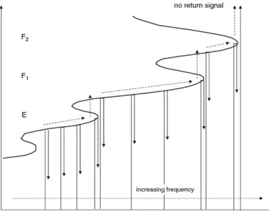
Each ionospheric layer has a different electron density maximum and thus its own critical frequency. Since the layer maxima increase progressively with altitude, a simple experiment can be designed to identify the critical frequencies and heights of each layer. If a pulse of electromagnetic energy is fired vertically into the ionosphere, initially a low (carrier) frequency, the pulse will be “reflected” off the lower portion of the E layer (the D region generally does not have enough ionization to cause refraction and so is ignored). As the frequency in increased, the pulse will be reflected from higher in the E layer until the E layer critical frequency is reached. Any further increase in frequency will cause the pulse to penetrate right through the E layer, and until reflected from the lower portion of the F1 layer, where the electron density is similar to the E layer maximum. Continuing to increase frequency will cause the pulse to penetrate further into the F1 layer before being reflected, until the critical frequency of the F1 layer is reached. Beyond this the pulse will completely penetrate the F1 layer and be reflected from the F2 layer at the level where the electron density is similar to the F1 maximum. A further increase in frequency will cause the pulse to be reflected from higher up in the F2 layer until, once again, its critical frequency is reached, after which the pulse passes through the F2 layer with no further possibility of being reflected back to Earth. Figure 10 represents this sequence schematically. This experiment is known as ionospheric sounding and the instrument used to carry it out is called an ionosonde. The graphic representation of the results is usually called an ionogram.

Figure 10. Schematic representation of a ionosonde experiment. From “Radio Wave Propagation. An Introduction for the Non-Specialist”, Richard

Figure 11 shows predicted results and a stylised set of what actual results might resemble. The latter diverge significantly from the predicted values near the critical frequencies, where the layer heights also tend towards infinity. Height measurements are indicated as virtual heights.

28

Figure 11. Expected vs actual results of an ionosonde experiment. From “Radio Wave Propagation. An Introduction for the Non-Specialist”, Richard

2.2.1 The virtual height of an ionospheric layer

In order to establish the speed of a wave travelling on the surface of the ocean or an electromagnetic wave, it is sufficient to lock on to a point of constant phase and observe how fast the point moves. A continuous sinusoidal waveform, represented by cos θ , is travelling if:

t z

θ ω β= − (2.9)

in which z is the spatial coordinate and β is the phase constant of the wave, given by

β ω με

=

By setting θ=constant, the velocity of the wave is:

1

z

t

ω

ν

β

με

∂

=

= =

∂

This is referred to as the phase velocity since this is the observed speed of movement of a point of constant phase. A continuous sinusoidal wave carries no information and has no time reference points or markers that could be used in an ionosonde experiment. The wave needs to be modulated before it is useful for a time delay experiment of this type. Measuring the time taken by a pulse from transmission to reception makes it possible to gauge the height of the reflecting layer. It should be noted that the modulated pulse does not necessarily travel at the phase velocity and first the velocity of the modulation envelope must be established. Processing pulse modulation is unnecessarily complicated and the required theory can be derived from one

29 of the simplest of all modulations, a double side band suppressed carrier (DSBSC). DSBSC signals exhibit just two side bands, one above and one below the carrier frequency. When travelling, this can be expressed as

(

)

(

)

cos

ω β

t

₋

z

₊

cos

ω

t

₋

β

z

That can be written as:

(

) (

)

2cos

_ω

t

₋

_β

z

cos

_{Δ − Δ}

_ω

t

_β

z

₂

,

₂

,

₂

,

₂

ω ω

β β

ω ω

β β

ω

=

+

β

=

+

Δ =

ω

−

Δ =

β

−

The second term in (2.13) (2.13) is the modulation carrying the information. If a point of constant phase in chosen on the modulation envelope then it can be seen that the speed at which the modulation travels is given by group

z

t

t

ω

ν

=

∂

=

∂

∂

∂

That is the group velocity.

These two velocity can be expressed in terms of the refractive index as:

,

c

nc

n

ν

=

ν

=

Although these results were derived for DSBSC, they can nevertheless by applied to any modulation. The results shown in Figure 11 can now be interpreted by noting that as frequency approaches the critical frequency of a layer, with the pulse penetrating ever further into the layer, the refractive index is seen to fall.; Equation (2.16) shows that this causes pulse modulation to drop below the speed of light, the empty space value. The critical frequency occurs at the electron density maximum and here the refractive index is zero, implying that the pulse velocity also falls to zero. Consequently, whenever the delay between transmission and reception of a pulse is used to try and establish the height of an ionospheric layer, the height will be overestimated if the assumption is made that the signal travels at the speed of light (as radio waves do in outer space), which is why this measurement is referred to as virtual height. The height appears to be infinite at the critical frequency because the group velocity approaches zero.

30

2.2.2 Vertical ionograms

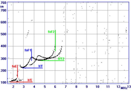
A typical ionogram recorded at a mid-latitude ionospheric station is shown in Figure 12. An ionogram records ionospheric conditions in terms of the relationship between a vertically emitted radio frequency and the virtual heights of echoes reflected from the ionosphere. The frequency range normally extends from about 1 to 20 MHz and the height range extends from 100 to 800 km. When the frequency range is near to the highest plasma frequency of the ionospheric layers, a split is observed in the radio echoes producing two traces, called the ordinary and extraordinary components and corresponding respectively to lower and higher frequency traces, separated by about half the electron gyro-frequency as a result of the influence of the geomagnetic field. At the critical frequencies of the ionospheric layers, the virtual height tends towards infinite, as already described above. For example, the ordinary wave critical frequency of the F2 layer, and the extraordinary wave critical frequency of the F1 layer are represented by foF2 and fxF1 respectively.

Ionogram height scales are marked on the assumption that radio waves propagate at the speed of light in the ionosphere,. while in reality they propagate more slowly in an ionized medium like the ionosphere. The recorded heights thus always tend to be higher than the real values and are referred to as virtual heights (h’), indicated as h’E, h’F etc. layer by layer.

Figure 12. Typical ionograms registered by AIS-INGV ionosonde installed in Rome.

An experienced operator can use ionograms to establish the most important ionospheric parameters, these being the critical frequency of the F2 layer (foF2), and the Maximum Usable Frequency at a distance of 3000

31 of ionograms In response to growing interest in real time mapping and short term forecasting. One example of a widely used and well tested automatic scaling program is the ARTIST system, developed at the University of Lowell, Center for Atmospheric Research.

2.2.3 Autoscala: software for automatic interpretation of the vertical ionograms

The INGV computer program AUTOSCALA implements an image recognition technique and does not require polarization information for operation, making it suitable for use with both single and crossed antenna systems. A maximum contrast technique is applied to a family of typical F2 layer shape functions and the nearest match is selected as representative of the current F2 layer trace. The vertical asymptote of the selected function represents the critical frequency foF2 and the MUF(3000)F2 is established numerically,

defining the tangential transmission curve to the selected function. The latest version of the INGV software introduces some important improvements.

1) Redesign of the main routine, reducing CPU footprint, and girofrequency parameterizing so that this version can scale ionograms recorded at any location.

2) It is not possible to scale the required ionospheric values (MUF(3000)F2 and foF 2) in a significant

proportion of ionograms for a variety of causes. These are well established and categorized in International Union of radio science (URSI) standards. The most frequent causes are:.

a) Blanketing by the E sporadic layer prevents observation of an F2 trace, when the URSI standard recommends using the descriptive letter A on bulletins to substitute the value of the ionospheric foF2

parameter.

b) The trace proximal to the critical frequency is not recorded clearly for various reasons, when the URSI standard recommends scaling the most probable foF2 value by extrapolation, extending the

traces hypothetically to the most likely critical frequency value. For extrapolated frequency ranges greater than 10%, the standard recommends reporting the highest recorded trace frequency followed by the qualifying letter D (greater than) and the appropriate descriptive letter explaining why the trace is unclearly defined (S interference, R absorption, C equipment). AUTOSCALA recognizes the trace and outputs both parameter values. In the latest version a method has been introduced and tested for identifying ionograms carrying insufficient information. This improvement means that ionograms assessed as lacking information are discarded by the program without generating any foF2 or MUF(3000)F2 data.

2.2.4 Adaptive Ionospheric Profiler (AIP)

The potential of the AUTOSCALA software was recently extended by the INGV team with the development of an algorithm for automatically estimating the electron density profile and adjusting the model parameters

32 according to ionogram readings. Other computer programs start from a scaled (manual or auto) ionogram trace, h′(f), and then derive a frequency profile for the plasma from the first frequency up to foF2. The new

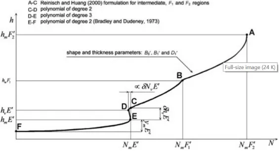
version of AUTOSCALA derives a limited number of parameters from an ionogram rather than a whole trace, and then surveys a range of possible versions to establish the profile that best matches the scaled parameters. The applied model is based on existing electron concentration models, which apply mathematical expressions to generate a profile based on ionospheric parameters scaled from ionograms. Figure 13 shows a diagram of the applied electron density profile model, which can be divided into two regions:

1. The bottom-side F2 profile, through the F1 layer to the top of the E valley (Figure 13, from A to C); 2. The E valley and the E bottom-side (Figure 13, from C to F)

Figure 13. The electron density model used in the INGV profiler(Scotto, 2009).

The models described above for the F2−F1 layer and E region can be used to construct an electron density profile with 12 free parameters (6 related to the E region and 6 to the F2− F1 layers). These 12 parameters are reported in Figure 13, and include:

1. NmF’2 maximum electron density of F2 layer

2. hmF’2 height of maximum electron density of F2layer

3. NmF’1 maximum electron density of F1 layer

4. B’0 thickness parameter

33 6. D’1 shape parameter

7. NmE’ maximum electron density of E layer

8. hmE’ height of maximum electron density of E layer

9. hvE’ height of E valley point

10. δ hvE’ E valley width

11. δ NvE’ E valley depth

12. ymE’ parabolic E layer semi-thickness

A flow chart of the algorithm is presented in Figure 14. An electron density profile is calculated from a model and this profile is then used to compute a simulated ionogram. The model parameters p are varied into appropriate Δp ranges centred in the vicinity of certain pbase values, referred to as “base values” and modelled

on the basis of the input data (external conditions parameters, geographic and geomagnetic coordinates of the station, foF2 and M(3000)F2). This provides a wide set of profiles, which in turn generate a corresponding

set of simulated ionograms, from among which the algorithm selects the ionogram that most resembles the recorded one. A range of variation must be selected for each p parameter also in consideration of the available computer resources. Generally speaking, the efficiency of the adjustment procedure is directly proportional to the variation range of the parameter, which in turn in directly proportional to computation time. The comparison between calculated and real ionograms represents the most critical phase for the algorithm and the choice of method has a marked effect on performance and computation time.

34

35

2.3

NeQuick model for ionospheric electron content

The NeQuick ionospheric electron density model was developed at the Aeronomy and Radiopropagation Laboratory of The Abdus Salam International Centre for Theoretical Physics (ICTP), in Trieste, Italy, and at the Institute for Geophysics, Astrophysics and Meteorology (IGAM) of the University of Graz, Austria. The evolution of NeQuick can be traced back to the DGR profiler proposed by Di Giovanni and Radicella in 1990 and modified by Radicella and Zhang in 1995. The European Space Agency (ESA) European Geostationary Navigation Overlay Service (EGNOS) project for assessment analysis implemented the original version of this model for single-frequency positioning applications within the framework of the European Galileo project. The International Telecommunication Union, Radiocommunication Sector (ITU-R) also adopted it as a suitable method for TEC modelling. The source code for NeQuick (FORTRAN 77) is available at

http://www.itu.int/ITU-R/. There has been significant work to improve the analytical formulation of NeQuick and to exploit the growing availability of data with continuous updating of the model. Specific modifications were made in response to the need to better represent the median ionosphere on a global scale. The bottomside and topside modelling descriptions have recently been subject to major changes. Specific revisions have also been introduced in the computer package associated with the NeQuick model to improve its computational efficiency. The main features of NeQuick2 are outlined below but first it is useful to recall the Epstein function expression that underlies the model formulation:

max max max max 2 max

4

(h,h , N ,B)

exp

1 exp

N

h h

N

B

h h

B

−





=



_



_





₋





+







_

_







2.3.1 Bottomside ionosphere modelling

Considering the well-known expressions relating maximum electron density and critical frequency (in 1011 m-3_{) for each ionospheric layer}

NmE

=

0.12 (

4

foE

)

NmF

1 0.12

=

4

(

foF

1

)

NmF

2 0.12

=

4

(

foF

2

)

and F2 layer thickness parameters (in km), respectively, it is possible to express the NeQuick 2 bottomside as a sum of semi-Epstein layers as follows:

1 2

(h)

(h)

(h)

(h)

N

=

N

+

N

+

N

4

*

(h)

exp

(h)

1 exp

(h)

N E

h h E

N

B

h h E

B

ξ

ξ



₋



=









₋









+















