2020-12-03T12:21:11Z
Acceptance in OA@INAF
The ALMA Spectroscopic Survey in the HUDF: Nature and Physical Properties of
Gas-mass Selected Galaxies Using MUSE Spectroscopy
Title
Boogaard, Leindert A.; DECARLI, ROBERTO; González-López, Jorge; van der
Werf, Paul; Walter, Fabian; et al.
Authors
10.3847/1538-4357/ab3102
DOI
http://hdl.handle.net/20.500.12386/28647
Handle
THE ASTROPHYSICAL JOURNAL
Journal
882
The ALMA Spectroscopic Survey in the HUDF: Nature and Physical Properties
of Gas-mass Selected Galaxies Using MUSE Spectroscopy
Leindert A. Boogaard1 , Roberto Decarli2 , Jorge González-López3,4 , Paul van der Werf1 , Fabian Walter5,6 , Rychard Bouwens1 , Manuel Aravena3 , Chris Carilli6,7 , Franz Erik Bauer4,8,9 , Jarle Brinchmann1,10 , Thierry Contini11 , Pierre Cox12, Elisabete da Cunha13 , Emanuele Daddi14 , Tanio Díaz-Santos3 , Jacqueline Hodge1 ,
Hanae Inami15,16, Rob Ivison17,18 , Michael Maseda1 , Jorryt Matthee19 , Pascal Oesch20 , Gergö Popping5 , Dominik Riechers5,21 , Joop Schaye1 , Sander Schouws1, Ian Smail22 , Axel Weiss23 , Lutz Wisotzki24, Roland Bacon15,
Paulo C. Cortes25,26 , Hans-Walter Rix5 , Rachel S. Somerville27,28, Mark Swinbank22, and Jeff Wagg29
1
Leiden Observatory, Leiden University, P.O. Box 9513, NL-2300 RA Leiden, The Netherlands;[email protected]
2
INAF–Osservatorio di Astrofisica e Scienza dello Spazio, via Gobetti 93/3, I-40129, Bologna, Italy
3
Núcleo de Astronomía de la Facultad de Ingeniería y Ciencias, Universidad Diego Portales, Av. Ejército Libertador 441, Santiago, Chile
4
Instituto de Astrofísica, Facultad de Física, Pontificia Universidad Católica de Chile Av. Vicuña Mackenna 4860, 782-0436 Macul, Santiago, Chile
5
Max Planck Institute für Astronomie, Königstuhl 17, D-69117 Heidelberg, Germany
6
National Radio Astronomy Observatory, Pete V. Domenici Array Science Center, P.O. Box O, Socorro, NM 87801, USA
7
Battcock Centre for Experimental Astrophysics, Cavendish Laboratory, Cambridge CB3 0HE, UK
8Millennium Institute of Astrophysics(MAS), Nuncio Monseñor Sótero Sanz 100, Providencia, Santiago, Chile 9
Space Science Institute, 4750 Walnut Street, Suite 205, Boulder, CO 80301, USA
10
Instituto de Astrofísica e Ciências do Espaço, Universidade do Porto, CAUP, Rua das Estrelas, PT4150-762 Porto, Portugal
11
Institut de Recherche en Astrophysique et Planétologie(IRAP), Université de Toulouse, CNRS, UPS, F-31400 Toulouse, France
12
Institut d’astrophysique de Paris, Sorbonne Université, CNRS, UMR 7095, 98 bis bd Arago, F-7014 Paris, France
13
Research School of Astronomy and Astrophysics, Australian National University, Canberra, ACT 2611, Australia
14
Laboratoire AIM, CEA/DSM-CNRS-Universite Paris Diderot, Irfu/Service d’Astrophysique, CEA Saclay, Orme des Merisiers, F-91191 Gif-sur-Yvette cedex, France
15
Univ. Lyon 1, ENS de Lyon, CNRS, Centre de Recherche Astrophysique de Lyon(CRAL) UMR5574, F-69230 Saint-Genis-Laval, France
16
Hiroshima Astrophysical Science Center, Hiroshima University, 1-3-1 Kagamiyama, Higashi-Hiroshima, Hiroshima, 739-8526, Japan
17
European Southern Observatory, Karl-Schwarzschild-Strasse 2, D-85748, Garching, Germany
18Institute for Astronomy, University of Edinburgh, Royal Observatory, Blackford Hill, Edinburgh EH9 3HJ, UK 19
Department of Physics, ETH Zurich, Wolfgang-Pauli-Strasse 27, 8093, Zurich, Switzerland
20
Department of Astronomy, University of Geneva, Ch. des Maillettes 51, 1290 Versoix, Switzerland
21
Cornell University, 220 Space Sciences Building, Ithaca, NY 14853, USA
22
Centre for Extragalactic Astronomy, Department of Physics, Durham University, South Road, Durham, DH1 3LE, UK
23
Max-Planck-Institut für Radioastronomie, Auf dem Hügel 69, D-53121 Bonn, Germany
24
Leibniz-Institut für Astrophysik Potsdam, An der Sternwarte 16, D-14482 Potsdam, Germany
25Joint ALMA Observatory—ESO, Av. Alonso de Córdova, 3104, Santiago, Chile 26
National Radio Astronomy Observatory, 520 Edgemont Road, Charlottesville, VA 22903, USA
27Department of Physics and Astronomy, Rutgers, The State University of New Jersey, 136 Frelinghuysen Road, Piscataway, NJ 08854, USA 28
Center for Computational Astrophysics, Flatiron Institute, 162 5th Avenue, New York, NY 10010, USA
29
SKA Organization, Lower Withington Macclesfield, Cheshire SK11 9DL, UK
Received 2018 December 21; revised 2019 March 18; accepted 2019 April 12; published 2019 September 11 Abstract
We discuss the nature and physical properties of gas-mass selected galaxies in the ALMA spectroscopic survey (ASPECS) of the Hubble Ultra Deep Field (HUDF). We capitalize on the deep optical integral-field spectroscopy from the Multi Unit Spectroscopic Explorer(MUSE) HUDF Survey and multiwavelength data to uniquely associate all 16 line emitters, detected in the ALMA data without preselection, with rotational transitions of carbon monoxide(CO). We identify 10 as CO(2–1) at 1<z<2, 5 as CO(3–2) at 2<z<3, and 1 as CO(4–3) at z=3.6. Using the MUSE data as a prior, we identify two additional CO(2–1) emitters, increasing the total sample size to 18. We infer metallicities consistent with(super-)solar for the CO-detected galaxies at z1.5, motivating our choice of a Galactic conversion factor between CO luminosity and molecular gas mass for these galaxies. Using deep Chandra imaging of the HUDF, we determine an X-ray AGN fraction of 20% and 60% among the CO emitters at z∼1.4 and z∼2.6, respectively. Being a CO-flux-limited survey, ASPECS-LP detects molecular gas in galaxies on, above, and below the main sequence (MS) at z∼1.4. For stellar masses 1010(1010.5) M, we detect about 40%(50%) of all galaxies in the HUDF at 1<z<2 (2<z<3). The combination of ALMA and MUSE integral-field spectroscopy thus enables an unprecedented view of MS galaxies during the peak of galaxy formation.
Key words: galaxies: high-redshift– galaxies: ISM – galaxies: star formation
1. Introduction
Star formation takes place in the cold interstellar medium (ISM) and studying the cold molecular gas content of galaxies is therefore fundamental for our understanding of the formation and evolution of galaxies. As there is little to no emission from the molecular hydrogen that constitutes the majority of the
molecular gas in mass, cold molecular gas is typically traced by molecules, such as the bright rotational transitions of12C16O (hereafter CO).
Recent years have seen a tremendous advance in the characterization of the molecular gas content of high-redshift galaxies (for a review, see Carilli & Walter 2013). Targeted
surveys with the Atacama Large Millimetre Array(ALMA) and the Plateau de Bure Interferometer (PdBI) have been instru-mental in our understanding of the increasing molecular gas reservoirs of star-forming galaxies at z>1 (Daddi et al. 2010, 2015; Genzel et al. 2010; Tacconi et al. 2010, 2013; Silverman et al. 2015, 2018). Combining data across cosmic time, these provide constraints on how the molecular gas content of galaxies evolves as a function of their physical properties, such as stellar mass (M*) and star formation rate (SFR; Tacconi et al. 2013, 2018; Scoville et al. 2014, 2017; Genzel et al. 2015; Saintonge et al. 2016). These surveys typically target galaxies with SFRs that are greater than or equal to the majority of the galaxy population at their respective redshifts and stellar masses (the “main sequence” of star-forming galaxies; Brinchmann et al.2004; Noeske et al. 2007; Whitaker et al. 2014; Schreiber et al. 2015; Boogaard et al. 2018; Eales et al. 2018), and therefore should be complemented by studies that do not rely on such a preselection.
Spectral line scans in the (sub)millimeter regime in deep fields provide a unique window into the molecular gas content of the universe. As the cosmic volume probed is well defined, these scans play a fundamental role in determining the evolution of the cosmic molecular gas density through cosmic time. Through their spectral scan strategy, these surveys are designed to detect molecular gas in galaxies without any preselection, providing aflux-limited view of the molecular gas emission at different redshifts(Decarli et al.2014,2016; Walter et al.2014,2016; Pavesi et al.2018; Riechers et al.2019). By conducting “spectroscopy-of-everything,” these can in princi-ple reveal the molecular gas content in galaxies that would not be selected in traditional studies(e.g., galaxies with a low SFR, well below the main sequence (MS), but with a substantial gas mass).
This paper is part of a series of papers presenting the first results from the ALMA Spectroscopic Survey Large Program (ASPECS-LP; Decarli et al. 2019). The ASPECS-LP is a spectral line scan targeting the Hubble Ultra Deep Field (HUDF). Here we use the results from the spectral scan of Band 3 (84–115 GHz; 3.6–2.6 mm) and investigate the nature and physical properties of galaxies detected in molecular emission lines by ALMA. In order to do so, it is important to know about the physical conditions of the galaxies detected in molecular gas, such as their ISM conditions, their (HST) morphology, and their stellar and ionized gas dynamics. The HUDF benefits from the deepest and most extensive multiwavelength data, and, recently, ultra-deep integral-field spectroscopy.
A critical step in identifying ALMA emission lines with actual galaxies relies on matching the galaxies in redshift. In this context, the Multi Unit Spectroscopic Explorer (MUSE; Bacon et al. 2010) HUDF survey, which provides a deep optical integral-field spectroscopic survey over the HUDF (Bacon et al.2017), is essential. The MUSE HUDF is a natural complement to the ASPECS-LP in the same area on the sky, providing optical spectroscopy for all galaxies within the field of view, also without any preselection. In addition, the integral-field spectrograph provides redshifts for over a thousand galaxies in the HUDF (increasing the number of previously known redshifts by a factor of ∼10×; Inami et al. 2017). Depending on the redshift, these data can provide key information on the ISM conditions (such as metallicity and
dynamics) of the galaxies harboring molecular gas. As we will see throughout this paper, the MUSE data are a significant step forward in our understanding of galaxy population selected with ALMA.
The paper is organized as follows: we first introduce the spectroscopic and multiwavelength data(Section2). We discuss the redshift identification of the CO-detected galaxies from the line search(Gonzalez-Lopez et al.2019), using the MUSE and multiwavelength data, in Section 3.1. Next, we leverage the large number of MUSE redshifts to separate real from spurious sources down to a significantly lower signal-to-noise ratio (S/N) than possible in the line search (Section 3.2). Together, these sources form the full ASPECS-LP Band 3 sample(Section3.3). We then move on to the central question(s) of this paper: by doing a survey of molecular gas, in what kinds of galaxies do we detect molecular gas emission at different redshifts, and what are the physical properties of these galaxies? We determine stellar masses, SFRs, and(where possible) metallicities for all sources in Section4and link these to the molecular gas content(Mmol) to derive the gas fraction(Mmol M*, the molecular-to-stellar mass ratio) and depletion time (tdepl=Mmol SFR). We first discuss the properties of the sample of CO-detected galaxies in the context of the overall population of the HUDF (Section 5.1) and investigate the X-ray AGN fraction among the detected sources(Section 5.2). Using the MUSE spectra, we determine the unobscured SFR (Section 5.3) and the metallicity of the 1<z<1.5 sources (Section 5.4). Finally, we discuss the CO-detected galaxies from theflux-limited survey in the context of the galaxy MS (Section 6), focusing on the molecular gas mass, gas fraction, and depletion time. We discuss what fraction of the galaxy population in the HUDF we detect with increasing redshift. A further discussion of the molecular gas properties of these sources will be presented in Aravena et al.(2019).
Throughout this paper, we adopt a Chabrier(2003) IMF and aflat ΛCDM cosmology, with H0=70 km s−1Mpc−1,Ωm=
0.3, andΩΛ=0.7. Magnitudes are in the AB system (Oke & Gunn1983).
2. Observations 2.1. ALMA Spectroscopic Survey
We focus on the ASPECS-LP Band 3 observations that have been completed in ALMA Cycle 4. The acquisition and reduction of the Band 3 data are described in detail in Decarli et al.(2019). Thefinal mosaic covers a 4.6arcmin2area in the HUDF(where the primary beam response is>50% of the peak sensitivity). The data are combined into a single spectral cube with a spatial resolution of ≈1 75×1 49 (synthesized beam with natural weighting at 99.5 GHz) and a spectral resolution of 7.813 MHz, corresponding to Δv≈23.5 km s−1 at 99.5 GHz. The average root-mean-square(rms) sensitivity is ≈0.2 mJy beam−1but varies across the frequency range, being deepest (≈0.13 mJy beam−1) around 100 GHz and higher above 110 GHz, due to the spectral setup of the observations (see Gonzalez-Lopez et al. 2019 for details). Throughout this paper, we consider the area that lies within>40% of the primary beam peak sensitivity, which is the shallowest part of the survey over which we still detect CO candidates without preselection(Section3.1). When comparing to the HST reference frame, we take into account an astrometric offset ofΔα=+0 076, Δδ=−0 279 (Rujopakarn et al.2016; Dunlop et al.2017).
We perform an extensive search of the cube for molecular emission lines, as is detailed in Gonzalez-Lopez et al. (2019) and Section3. With the Band 3 data alone, the ASPECS-LP is sensitive to different CO and[C I] transitions at specific redshift ranges, which are indicated in the top panel of Figure1.
2.2. MUSE HUDF Survey
The HUDF was observed with the MUSE as part of the MUSE Hubble Ultra Deep Field survey (Bacon et al. 2017). The location on the sky of the ASPECS-LP with respect to the MUSE HUDF is shown in Decarli et al.(2019), Figure1. The MUSE integral-field spectrograph has a 1′×1′ field of view, covering the optical regime (4750–9300 Å) at an average spectral resolution ofλ/Δλ≈3000. The HUDF was observed in a two-tier strategy, with the mosaic-region reaching a median depth of 10 hr in a 3′×3′ region and the udf10-pointing reaching 31 hr depth in a 1′×1′ region (3σ emission line depth for a point source of 3.1 and 1.5×10⁻¹⁹erg s−1cm−2 at 7000Å, respectively). The data acquisition and reduction as well as the automated source detection are described in detail in Bacon et al. (2017). The measured seeing in the reduced data cube is 0 65 full width at half maximum(FWHM) at 7000 Å. Redshifts were identified semiautomatically and the full spectroscopic catalog is presented in Inami et al. (2017). The spectra were extracted using a weighted extraction, where the weighting was based on the MUSE white light image, to obtain the maximal signal-to-noise. The spectra are modeled with a
modified version ofPLATEFIT(Brinchmann et al.2004,2008; Tremonti et al. 2004) to obtain line-flux measurements and equivalent widths for all sources. The typical uncertainty on the redshift measurement is σv=0.00012(1+z) or ≈40 km s−1
(Inami et al.2017), which we use to compute the uncertainties in the relative velocities.
In order to compare in detail the relative velocities measured between the UV/optical features in MUSE and CO in ALMA, we need to place both on the same reference frame. The MUSE redshifts are provided in the barycentric reference frame, while the ALMA cube is set to the kinematic local standard of rest (LSRK). When determining detailed velocity offsets we place both on the same reference frame by removing the velocity difference; BARY−LSRK=−16.7 km s−1 (accounting for the angle between the LSRK vector and the observation direction toward the HUDF).
The redshift distribution of the MUSE galaxies that fall within >40% of the primary beam peak sensitivity of the ASPECS-LP footprint in the HUDF is shown in Figure 1, where galaxies are color coded by the primary spectral feature(s) used to identify the redshift (see Inami et al. 2017 for details). The redshifts that correspond to the ASPECS band 3 coverage of the different molecular lines are indicated in the top panel. CO(1–0) [115.27 GHz] is observable at the lowest redshifts (z<0.3694), where MUSE still covers a major part of the rest-frame optical spectrum that contains a wealth of spectral features, including absorption and (strong) emission lines (e.g., Ha l6563,
l
O III 4959, 5007
[ ] , and[O II]l3726, 3729). The strong lines are the main spectral features used to identify star-forming galaxies all the way up to z<1.50, where[O II]l3726, 3729moves out of the spectral range of MUSE. CO(2–1)[230.54 GHz] is covered by ASPECS at 1.0059<z<1.7387, mostly overlapping with
O II
[ ] in MUSE. At z>1.5, the main features used to identify these galaxies are absorption lines such as Mg II l2796, 2803 and Fe IIl2586, 2600. Over the redshift range of CO(3–2) [345.80 GHz], 2.0088<z<3.1080, MUSE only has coverage of weaker UV emission lines(mainlyC III]l1907, 1909), making redshift identifications more challenging (the “redshift desert”). Here, UV absorption lines are commonly used to identify redshifts, for galaxies where the continuum is strong enough (mF775W
26 mag). Above z=2.9, MUSE flourishes again, with the coverage of Lyα λ1216 all the way out to z≈6.7. Here, ASPECS covers CO(4–3)[461.04 GHz] and transitions with Jup 4, and atomic carbon lines ([C I]1 0- 610μm and[C I]2 1 -370μm).
2.3. Multiwavelength Data(UV–Radio) and MAGPHYS
In order to construct spectral energy distributions(SEDs) for the ASPECS-LP sources, we utilize the wealth of available photometric data over the HUDF, summarized below.
We use the photometric compilation by Skelton et al.(2014, see references therein), which includes UV, optical, and near-IR photometry from the Hubble Space Telescope (HST) and ground-based facilities, as well as (deblended) Spitzer/IRAC 3.6, 4.5, 5.8, and 8.0μm. We also include the corresponding deblended Spitzer/MIPS 24 μm photometry from Whitaker et al. (2014). We take deblended far-infrared (FIR) data from Herschel/PACS 100 and 160 μmfrom Elbaz et al. (2011), which have a native resolution of 6 7 and 11 0, respectively. The PACS 100 and 160μm have a 3σ depth of 0.8 and 2.4 mJy and are limited by confusion. For theflux uncertainties we use the maximum of the local and simulated noise levels for each Figure 1.Molecular line redshift coverage of the galaxies in the MUSE and
ASPECS-LP Hubble Ultra Deep Field (HUDF). The histogram shows the galaxies with spectroscopic redshifts from MUSE (udf10 and mosaic; see Section 2.2) that lie within >40% of the primary beam sensitivity of the ASPECS-LP mosaic, distinguished by the primary spectral feature used to identify the redshift(Inami et al.2017;“Nearby galaxy” summarizes a range of rest-frame optical features). The decrease in the number of redshifts between 1.5<z<2.9 is due to the lack of strong emission line features in the MUSE spectrograph(“redshift desert”). The drop at the lowest redshifts is due to the nature and volume of the HUDF. The top panel shows the specific CO and C I[ ] transitions covered by the frequency setup of ASPECS Band 3 at different redshifts(Walter et al.2016; Decarli et al.2019). ASPECS covers CO(2–1) for
O II
[ ] emitters and absorption line galaxies at 1.0<z<1.74. Galaxies with CO(3–2) at 2.0<z<3.11 are identified mostly by UV absorption and weaker emission lines(e.g., C III]). For higher-order CO and C I[ ] transitions above z>2.90, MUSE has coverage ofLy .a
source, as recommended by the documentation.30 We further include the 1.2 mm continuum data from the combination of the available ASPECS-LP data with the ALMA observations by Dunlop et al.(2017), taken over the same region, as detailed in Aravena et al. (2019). We also include the ASPECS-LP 3.0 mm continuum data, as presented in Gonzalez-Lopez et al. (2019). For the ASPECS survey we have created a master photometry catalog for the galaxies in the HUDF, adopting the spectroscopic redshifts from MUSE(Section2.2) and literature sources, as detailed in Decarli et al.(2019).
We use the high-z extension of the SED-fitting code
MAGPHYS to infer physical parameters from the photometric information of the galaxies in our field (Da Cunha et al. 2008, 2015). The high-z extension of MAGPHYS includes a larger library of spectral emission models that extend to higher dust optical depths, higher SFRs and younger ages compared to what is typically found in the local universe. From the spectral emission models, the code can constrain the stellar mass, sSFR, and dust attenuation (AV) along the line of sight. An
energy-balance argument ensures that the amount of absorption at rest-frame UV/optical wavelengths is consistent with the light reradiated in the infrared. The code performs a Bayesian inference of the posterior likelihood distribution of the fitted parameter, to account for uncertainties such as degeneracies in the models, missing data, and nondetections.
We runMAGPHYS on all the galaxies in our catalog, using the available photometric information in all the bands(listed in Appendix B). We do not include the Spitzer/MIPS and Herschel/PACS photometry in the fits of the general sample because the angular resolution of these observations is relatively modest (>5″), thus a delicate deblending analysis would be required (the average sky density of galaxies in the HUDF is 1 galaxy per 3 arcsec2). For the CO-detected galaxies we repeat the MAGPHYS fits including these bands
(Section4.1). In order to take into account systematic errors in the zero-point fitting for these sources, we add the zero-point errors(Skelton et al.2014) in quadrature to the flux errors in all filters except HST, and include a 5% error-floor to further account for systematic errors in the physical models(following Leja et al. 2018). The filter selection of the general sample provides excellent photometric coverage of the stellar popula-tion. Paired with the wealth of spectroscopic redshifts (see Decarli et al. 2019 for a detailed description), this enables robust constraints on properties such as M*, SFR, and AV. We
do note that while the formal uncertainties on the inferred properties are generally small, systematic uncertainties can be of order ∼0.3dex (e.g., Conroy2013).
2.4. X-Ray Photometry
To identify AGN in thefield, we use the Chandra X-ray data available over the GOODS-S region from Luo et al. (2017), which reaches the full depth of 7 Ms over the HUDF area. In total, there are 36 X-ray sources within the ASPECS-LP region of the HUDF (i.e., within 40% of the primary beam). We spatially cross-match the X-ray catalog to the closest source within 1″in our MUSE and multiwavelength catalog over the ASPECS-LP area, visually inspecting all matches used in this paper to ensure they are accurately identified.
At the depth of the X-ray data, there are multiple physical mechanisms(e.g., AGN and star formation) that may produce the X-ray emission detected at 0.5–7 keV. Luo et al. (2017) adopt the following six criteria to distinguish X-ray AGN from other sources of X-ray emission, of which at least one needs to be satisfied to be classified as AGN (we refer the reader to Xue et al.2011; Luo et al.2017and references therein for details): (1) LX 3×1042 erg s−1, identifying luminous X-ray
sources; (2) an effective photon index Γeff1.0 indicating
hard X-ray sources, identifying obscured AGN;(3) X-ray-to-R-band flux ratio of log(fX fR)> -1; (4) spectroscopically classified as AGN via, e.g., broad emission lines and/or high excitation lines; (5) X-ray-to-radio flux ratio ofLX L1.4 GHz
´
2.4 1018, indicating an excess of X-ray emission over the level expected from pure star formation; and (6) X-ray-to-K-bandflux ratio oflog(fX fKs)> -1.2. Note that even with these criteria it is possible that some X-ray sources host low-luminosity or heavily obscured AGN and are currently misclassified.
Overall, there are six X-ray AGN in the ASPECS-LP volume at 1.0<z<1.7, all of which have a MUSE redshift (one being a broad-line AGN). In the ASPECS-LP volume at 2.0<z<3.1, there are seven X-ray AGN, three of which have spectroscopic redshifts from MUSE(including one broad-line AGN), and four with a photometric redshift (we discard one source in the catalog with a photometric redshift in this regime for which we cannot securely identify a counterpart in HST). There is one X-ray AGN at a higher redshift, which is also identified by MUSE as a broad-line AGN at z=3.188.
3. The ASPECS-LP Sample 3.1. Identification of the Line Search Sample
An extensive description of the line search is provided in Gonzalez-Lopez et al. (2019). In summary, three independent methods were combined to search for CO lines in the ASPECS-LP band 3 data without any preselection: LINESEEKER
(González-López et al. 2017), FINDCLUMP (Decarli et al.
2014; Walter et al.2016), andMF3D(Pavesi et al.2018). The fidelity31of these line candidates was estimated from the ratio of the number of lines with a negative and positive flux detected at a given S/N. Lastly, the completeness of the sample was estimated by ingesting simulated emission lines into the real data cube.
In total, there are 16 emission line candidates for which the fidelity is 0.9. Statistical analysis shows that this sample is free from false positives(the sum of their fidelities, based on the ALMA data alone, is 15.9; Gonzalez-Lopez et al. 2019). These 16 sources form the primary, line search sample and are shown in Figure2. All these candidates have an S/N 6.4.
For all sources in the primary sample, one or multiple potential counterpart galaxies are visible in the deep HST imaging shown in Figure2. In order to confidently identify a single CO emission line, an independent redshift measurement of the potential counterpart measurement is needed. Given the wealth of multiwavelength photometry in the HUDF, photo-metric redshifts can often already provide sufficient constraints to discern between different rotation transitions of CO in the case of isolated galaxies at redshifts z 3. However, complex systems of several galaxies, or projected superpositions of
30
https://hedam.lam.fr/GOODS-Herschel/data/files/documentation/ GOODS-Herschel_release.pdf
31
Thefidelity is defined as F=1−P, where P is the probability of a line being produced by noise(Gonzalez-Lopez et al.2019).
independent galaxies at distinct redshifts, can make redshift assignments more complicated. Fortunately, the integral-field spectroscopy from MUSE is ideally suited to disentangle spectral features belonging to different galaxies, allowing us to confidently assign redshifts to the CO emission lines. The
frequency of a CO line can correspond to different rotational transitions, each with a unique associated redshift. With the potential redshift solutions in hand, we systematically identify the CO line candidates from the line search. We provide a summary of the redshift identifications here. A detailed Figure 2. HSTRGB cutouts(F160W, F125W, and F105W) of the 16 CO line detections from the line search, all revealing an optical/NIR counterpart. Each panel is 8″×8″ centered around the CO emission (corrected astrometry; Section2.1). The white contours indicate the CO signal from ±[3, .., 11]σ in steps of 2σ. The ALMA beam is indicated in the bottom left corner. Galaxies with a spectroscopic redshift from MUSE(Inami et al.2017) matching the CO signal are labeled in green (and red if not matching); spectroscopic redshifts in blue are newly determined in this paper. Of the 16 galaxies, 12 match closely to a redshift from MUSE (including ASPECS-LP.3mm.08, discussed in AppendixAand Decarli et al.2016). ASPECS-LP.3mm.03, 3mm.07, and 3mm.09 have mF775W>27, which is too faint for a direct absorption line redshift from MUSE(but are independently confirmed). For ASPECS-LP.3mm.09 we do find UV absorption features matching the CO(3–2) in the galaxy slightly to the north. A new absorption line redshift is found for ASPECS-LP.3mm.12(see Figure18). The photometric redshift and absence of lower-z spectral features indicate ASPECS-LP.3mm.13 being at z=3.601.
description of the individual sources and their redshift identifications can be found in Appendix A, where we also show the MUSE spectra for all sources (Figures13–16).
First, we correlate the spatial position and potential redshifts of the CO lines with known spectroscopic redshifts from MUSE(Inami et al.2017). From the MUSE redshifts alone, we immediately identify most (11/16) of the CO lines with the highest fidelity. The brightest (ASPECS-LP.3mm.01) is a CO(3–2) emitter at z=2.54, showing a wealth of UV absorption features. The other 10 galaxies are a diverse sample of CO(2–1) emitters spanning the redshift range over which we are sensitive: 1.01<z<1.74. They show a variety of spectra at different levels of S/N, covering a range of UV and optical absorption and emission features. Notably,[O II]l3726, 3729 is detected in all galaxies where it is covered by MUSE, while
l Ne III 3869
[ ] is detected in some of the higher S/N spectra. Next, we extract MUSE spectra for the remainingfive (5/16) sources without a cataloged redshift and investigate their spectra for a redshift solution matching the observed CO line. We discover two new spectroscopic redshifts at z= 2.54 (ASPECS-LP.3mm.12) and z=2.69 (associated with ASPECS-LP.3mm.09) confirming detections of CO(3–2), which were both not included in the catalog of Inami et al. (2017) as their spectra are blended with foreground sources. The former in particular demonstrates the key use of MUSE in disentangling a spatially overlapping system comprised of a foreground O II[ ] emitter and a faint background galaxy, which is detected at S/N>4 both via cross-correlation with a z≈2.5 spectral template and by stacking absorption features (see Figure 18). For LP.3mm.03 and ASPECS-LP.3mm.07 we leverage the absence of spectral features (e.g., O II[ ], Lya), consistent with their faint magnitudes (mF775W>27 mag) and a redshift in the MUSE redshift desert,
in combination with photometric redshifts in the z=2–3 regime from the deep multiwavelength data, to confirm detections of CO(3–2). Lastly, we find ASPECS-LP.3mm.13 being CO(4–3) at z=3.601, based on the photometric redshifts suggesting z≈3.5 and the absence of a lower redshift solution from the spectrum. Lyα λ1216 is not detected for this source, but we caution that at this redshift Lya falls very close to the[O I]l5577skyline. Furthermore, given that the source potentially contains significant amounts of dust, no
a
Ly emission may be expected at all.
In summary, we determine a redshift solution for all(16/16) candidates from the line search. Twelve are directly confirmed by MUSE spectroscopy, while the remaining four are supported by their photometric redshifts and indirect spectro-scopic evidence. We highlight that some of these counterparts are very faint, even in the reddest HST bands, and their identifications would not have been possible without the exquisite depth of both the HST and MUSE data over the HUDF. Similar objects would typically not have robust photometric counterparts in areas of the sky with inferior coverage (let alone have independent spectroscopic confirmation).
The identifications of the CO transitions, along with their MUSE counterparts, are presented in Table 1. We show the spatial extent of the CO emission on top of the HST images in Figure 2. The MUSE spectra for the individual sources are shown in Figures13–16and discussed in AppendixA.
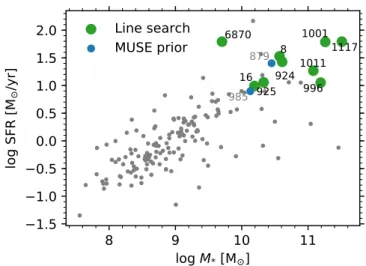
3.2. Additional Sources with MUSE Redshift Priors at z<2.9 The CO-line detections from Gonzalez-Lopez et al. (2019) are selected to have the highest fidelity and are therefore the highest S/N ( 6.4) candidates over the ASPECS-LP area. In Figure3, we plot the stellar mass–SFR relation for all MUSE sources at 1.01<z<1.74, where we indicate all the galaxies that have been detected in CO(2–1) in the line search.32There are several galaxies in the field with properties similar to the ASPECS-LP galaxies that are not detected in the line search. This raises the following question: why are these galaxies not detected? Given their physical properties, we may expect some of these galaxies to harbor molecular gas and therefore to have CO signal in the ASPECS-LP cube. The reason that we did not detect these sources in the line search may, therefore, simply be due to the fact that they are present at lower S/N, which puts them in the regime where the decreasing fidelity makes it challenging to identify them among the spurious sources.
However, the physical properties of the galaxies themselves provide an extra piece of information that can guide us in detecting CO for these sources. In particular, we can use the spectroscopic redshifts from MUSE to obtain a measurement of the CO flux for each source, either identifying them at lower S/N, or putting an upper limit on their molecular gas mass. We aim at the CO transitions covered at z<2.9, where the features in the MUSE spectrum typically provide a systemic redshift. At higher redshift the main spectral feature used to identify redshifts is oftenLy , which can be offset from the systemica redshift by a few hundred km s−1 (e.g., Shapley et al. 2003; Rakic et al.2011; Verhamme et al.2018).
We extract a single-pixel spectrum from the 3″ tapered cube at the position of each MUSE source in the redshift range, after correcting for the astrometric offset (Section2.1). We then fit
Figure 3.Stellar mass vs. SFR(from MAGPHYS) of all galaxies with a MUSE redshift at 1.01< <z 1.74 in the ASPECS-LP footprint. Leveraging the MUSE redshift as prior, wefind a CO(2–1) signal in two additional galaxies (blue). The numbers indicate the MUSE IDs of the sources. The detections from the line search(green; Section3.1) are also recovered in the prior-based search. By using the MUSE redshifts to search for CO at lower luminosities, we reveal molecular gas in most of the massive, star-forming galaxies at these redshifts.
32
Note that we do not show the MUSE source associated with ASPECS-LP.3mm.08 and the two MUSE sources that are severely blended with ASPECS-LP.3mm.12 and the galaxy north of ASPECS-LP.3mm.09 on the plot.
the lines with a Gaussian curve, using a custom-made Bayesian Markov chain Monte Carlo routine with the following priors:
1. line peak velocity: a Gaussian distribution centered at Δv=0 (based on the MUSE redshift) and σ= 100 km s−1(the MUSE spectral resolution).
2. line width: a Maxwellian distribution with a width of 100 km s−1.
3. line flux: a Gaussian distribution centered at zero, with σ=0.5 Jy km s−1, allowing both positive and negative
line fluxes to be fitted.
We choose a strong prior on the velocity difference, as we only search for lines at the exact MUSE redshift. The Gaussian prior on the line flux is important to estimate the fidelity of our measurements, allowing an unbiased comparison of positive versus negative linefluxes (see Gonzalez-Lopez et al.2019for details). The Maxwellian prior is chosen because it is bound to produce positive values of the line width, depends on a single scale parameter, and has a non-null tail at very large line widths. The uncertainties are computed from the 16th and 84th percentiles of the posterior distributions of each parameter.
As narrow lines are more easily caused by noise in the cube (Gonzalez-Lopez et al. 2019), we rerun the fit with a broader prior on the line width of 200 km s−1. We also independentlyfit the spectrum with a uniform prior over ±1GHz around the MUSE redshift. We select only the sources in which the same feature was recovered with S/N>3 in all three fits. In order to select a sample that is as pure as possible, we select only the objects that have a velocity offset of<80 km s−1from the MUSE systemic redshift (≈×2 the typical uncertainty on the MUSE redshift). In addition, we only keep objects with a line width of>100 km s−1, to avoid including spurious narrow lines. We note that, while these cuts potentially remove other sources that are detected at lower S/N, we do not attempt to be
complete. Rather, we aim to have the prior-based sample as clean as possible.
The prior-based search reveals two additional sources detected in CO(2–1) with an S/N>3 (see Table 2). Both sources lie within the area in which the sensitivity is>40% of the primary beam peak sensitivity. We show the HST cutouts with the CO spectra of these sources in Figure 4, ordered by S/N. ASPECS-LP-MP.3mm.02 is the foreground spiral galaxy of ASPECS-LP.3mm.08. This source was already found in the ASPECS-Pilot(Decarli et al.2016, see AppendixA).
Because the molecular gas mass is tofirst order correlated with the SFR, we expect to detect CO in the galaxies with the highest SFRs at a given redshift. Sorting all the galaxies by their SFR indeed reveals a clear correlation between the SFR and the S/N in CO, suggesting there are additional sources in the ASPECS-LP data cube at lower S/N. This can also be clearly seen from Figure3, where our stringent sample of prior-based sources all lie at log SFR[Myr−1]>0.5. Qualitatively, it becomes clear that the ASPECS-LP is sensitive enough to detect molecular gas in most massive MS galaxies at 1.01<z<1.74 (a quantitative discussion of the detection fraction for the full sample is provided in Section6). For many galaxies, the reason these are not unveiled in the line search may simply be because their lower CO luminosity and/or smaller line width puts them below the conservative S/N threshold we adopt in the line search. Using the MUSE redshifts as prior information, it is possible to unveil their molecular gas reservoirs at lower S/N.
3.3. Full Sample Redshift Distribution
The full ASPECS-LP CO line sample consists of 18 galaxies with a CO detection in the HUDF; 16 detections without preselection and 2 MUSE redshift prior-based detections. Table 1
ASPECS-LP CO-detected Sources from the Line Search, with MUSE Spectroscopic Counterparts
ID R.A. Decl. νCO CO trans. zCO MUSE ID zMUSE Δv
(J2000) (J2000) (GHz) (JupJlow) (km s−1) (1) (2) (3) (4) (5) (6) (7) (8) (9) 3mm.01 03:32:38.54 −27:46:34.6 97.584±0.003 3→2 2.5436 35 2.5432 −15.5±41.0 3mm.02 03:32:42.38 −27:47:07.9 99.510±0.005 2→1 1.3167 996 1.3172a 73.5±42.7 3mm.03 03:32:41.02 −27:46:31.5 100.131±0.005 3→2 2.4534 L L L 3mm.04 03:32:34.44 −27:46:59.8 95.501±0.006 2→1 1.4140 1117 1.4147 102.9±44.2 3mm.05 03:32:39.76 −27:46:11.5 90.393±0.006 2→1 1.5504 1001 1.5509 71.7±44.7 3mm.06 03:32:39.90 −27:47:15.1 110.038±0.005 2→1 1.0951 8 1.0955 79.2±42.3 3mm.07 03:32:43.53 −27:46:39.4 93.558±0.008 3→2 2.6961 L L L 3mm.08 03:32:35.58 −27:46:26.1 96.778±0.002 2→1 1.3821 6415 1.3820 −0.1±40.5 3mm.09 03:32:44.03 −27:46:36.0 93.517±0.003 3→2 2.6977b L L L 3mm.10 03:32:42.98 −27:46:50.4 113.192±0.009 2→1 1.0367 1011 1.0362a −53.7±46.6 3mm.11 03:32:39.80 −27:46:53.7 109.966±0.003 2→1 1.0964 16 1.0965 19.8±40.8 3mm.12 03:32:36.21 −27:46:27.7 96.757±0.004 3→2 2.5739 1124c 2.5739a 16.8±41.9 3mm.13 03:32:35.56 −27:47:04.3 100.209±0.006 4→3 3.6008 L L L 3mm.14 03:32:34.84 −27:46:40.7 109.877±0.009 2→1 1.0981 924 1.0981 15.0±46.9 3mm.15 03:32:36.48 −27:46:31.9 109.971±0.005 2→1 1.0964 6870 1.0979 240.4±42.3 3mm.16 03:32:39.92 −27:46:07.4 100.503±0.004 2→1 1.2938 925 1.2942 66.3±41.7
Notes.The CO frequencies are taken from Gonzalez-Lopez et al.(2019). (1) ASPECS-LP 3mm ID. (2)–(3) Coordinates. (4) CO line frequency. (5) Identified CO transition(Section3.1). (6) CO redshift. (7) MUSE ID. (8) MUSE redshift. (9) Velocity offset between MUSE and ALMA (D =v (zMUSE-zCO) (1+zCO) after; converting both to the same reference frame).
a
Updated from Inami et al.(2017), see AppendixA.
b
Additionally supported by matching absorption found in MUSE#6941, at z=2.695, 0 7 to the north.
c
These galaxies span a range of redshifts between 1<z<4. The lowest redshift galaxy is detected in CO(2–1) at z=1.04, while the highest redshift galaxy is detected(without prior) in CO(4–3) at z=3.60. We show a histogram of the redshifts of the line-search and prior-based detections in Figure 5.
Twelve sources are detected in CO(2–1) at 1.01<z<1.74, where the combination of molecular line sensitivity and survey volume are optimal. Most prominently, we detectfive galaxies at the same redshift of z≈1.1. These galaxies are all part of an overdensity of galaxies in the HUDF at z=1.096, visible in Figure1.
Five sources are detected in CO(3–2) at 2.01<z<3.11, including the brightest CO emitter in the field at z=2.54 (ASPECS-LP.3mm.01; see also Decarli et al.2016) and a pair of galaxies (ASPECS-LP.3mm.07 and #9) at z≈2.697 (see Section 3.1). All five CO(3–2) sources are detected in 1 mm dust continuum(Aravena et al.2016; Dunlop et al.2017) with flux densities below 1mJy. However, only one of these sources (ASPECS-LP.3mm.01) previously had a spectroscopic redshift (Walter et al.2016; Inami et al. 2017).
4. Physical Properties 4.1. SFRs from MAGPHYSand [OII]
For all the CO-detected sources, we derive the SFR(and M* and AV) from the UV-FIR data (including 24–160 μm
and ASPECS-LP 1.2 and 3.0 mm) using MAGPHYS (see
Section2.3), which are provided in Table3. The full SEDfits are shown in Figure19.
For the 1<z<1.5 subsample, we have access to the O II[ ] l3726, 3729-doublet. We derive SFRs from[O II]l3726, 3729 following Kewley et al.(2004), adopting a Chabrier (2003) IMF. The observed [O II] luminosity gives a measurement of the unobscured SFR, which can be compared to the total SFR (including the FIR) to derive the fraction of obscured star formation. For that reason, we do not apply a dust correction when calculating the SFR( O II[ ]).
The derived SFR([O II]l3726, 3729) is dependent on the oxygen abundance. We have access to the oxygen abundance directly for some of the sources and can also make an estimate through the mass–metallicity relation (e.g., Zahid et al. 2014). However, because of the additional uncertainties in the calibrations for the oxygen abundance, we instead adopt an average[O II]l3726, 3729/ aH ratio of unity, given that all our sources are massive and hence expected to have high oxygen abundance 12+log O H∼8.8, where [O II] Ha =1.0 Table 2
ASPECS-LP CO(2–1) Detected Sources Based On a Spectroscopic Redshift Prior from MUSE
ID R.A. Decl. νCO CO trans. zCO MUSE ID zMUSE Δv
(J2000) (J2000) (GHz) (JupJlow) (km s−1)
(1) (2) (3) (4) (5) (6) (7) (8) (9)
MP.3mm.01 03:32:37.30 −27:45:57.8 109.978±0.011 2→1 1.0962 985 1.0959 −28.2±50.6
MP.3mm.02 03:32:35.48 −27:46:26.5 110.456±0.007 2→1 1.0872 879 1.0874 55.8±44.3
Note.(1) ASPECS-LP MUSE prior (MP) ID. (2)–(3) Coordinates. (4) CO line frequency. (5) CO transition. (6) CO redshift. (7) MUSE ID. (8) MUSE redshift. (9) Velocity offset between MUSE and ALMA (D =v (zMUSE-zCO) (1+zCO) after converting both to the same reference frame).;
Figure 4. HSTcutouts(F160W, F125W, and F105W) and CO(2–1) spectra for two additional CO line candidates, found through a MUSE redshift prior. The CO contours are shown in white starting at±2σ in steps of 1σ. All other labeling in the cutouts is the same as that in Figure3. In the spectra the velocity is given relative to the MUSE redshift. The spectrum and best-fit Gaussian are shown in black and red, respectively. The local rms noise level is shown in green.
Figure 5.Redshift distribution of the ASPECS-LP CO-detected sources, which all have an HST counterpart. We show both the detections from the line search (Section3) as well as the MUSE prior-based galaxies (Section3.2). The gray shading indicates the redshift ranges over which we can detect different CO transitions.
(e.g., Kewley et al. 2004). For all galaxies with S/N ([O II]l3726, 3729)>3, excluding the X-ray AGN, the
l +l
O II 3726 3729
[ ] line flux measurements and SFRs are
presented in Table4.
4.2. Metallicities
It is well known that the gas-phase metallicity of galaxies is correlated with their stellar mass, with more massive galaxies having higher metallicities on average (e.g., Tremonti et al. 2004; Maiolino et al.2008; Mannucci et al.2010; Zahid et al. 2014). For the 1.0<z<1.42 subsample, we have access to
l Ne III 3869
[ ] , which allows us to derive a metallicity from l
Ne III 3869
[ ] /[O II]l3726, 3729. We follow the relation as presented by Maiolino et al. (2008), who calibrated the
Ne III
[ ]/ O II[ ] line ratio against metallicities inferred from the direct Te method (at low metallicity; 12+log O H<8.35)
and theoretical models from Kewley & Dopita(2002; at high metallicity, mainly relevant for this paper;12+log O H> 8.35). Since the wavelengths of [Ne III]l3869 and [O II] l3726, 3729 are close, this ratio is practically insensitive to dust attenuation. The physical underpinning lies in the fact that the ratio of the low-ionization[O II] and high-ionization
Ne III
[ ] lines is a solid tracer of the shape of the ionizationfield, given that neon closely tracks the oxygen abundance(e.g., Ali et al.1991; Levesque & Richardson2014; Feltre et al.2018). As the ionization parameter decreases with increasing stellar metallicity(Dopita et al.2006a,2006b) and the metallicity of the young ionizing stars and their birth clouds is correlated, the ratio of[Ne III]l3869/[O II]l3726, 3729is a reasonable gas-phase metallicity diagnostic, albeit indirect, with significant scatter(Nagao et al.2006; Maiolino et al.2008) and sensitive to model assumptions(e.g., Levesque & Richardson2014). If
Table 3
Physical Properties of the ASPECS-LP Sources from the Line Search and the MUSE Prior-based Search, with Formal Uncertainties
ID z logM*,SED SFRSED AV ,SED X-ray XID
(M) (Myr−1) (mag) (1) (2) (3) (4) (5) (6) (7) ASPECS-LP.3mm.01 2.5436 10.4-+0.00.0 233-+00 2.7-+0.00.0 AGN 718 ASPECS-LP.3mm.02 1.3167 11.2-+0.00.0 11+-02 1.7-+0.00.1 ASPECS-LP.3mm.03 2.4534 10.7-+0.10.1 68-+2019 3.1-+0.30.1 ASPECS-LP.3mm.04 1.4140 11.3-+0.00.0 61+-123 2.9-+0.00.1 ASPECS-LP.3mm.05 1.5504 11.5-+0.00.0 62+-195 2.3-+0.30.1 AGN 748 ASPECS-LP.3mm.06 1.0951 10.6-+0.00.0 34+-00 0.8-+0.00.0 X 749 ASPECS-LP.3mm.07 2.6961 11.1-+0.10.1 187+-1635 3.2-+0.10.1 ASPECS-LP.3mm.08 1.3821 10.7-+0.00.0 35+-58 0.9-+0.10.1 ASPECS-LP.3mm.09 2.6977 11.1-+0.00.1 318-+3535 3.6-+0.10.1 AGN 805 ASPECS-LP.3mm.10 1.0367 11.1-+0.10.0 18-+11 3.0-+0.10.0 ASPECS-LP.3mm.11 1.0964 10.2-+0.00.0 10+-10 0.8-+0.10.0 ASPECS-LP.3mm.12 2.5739 10.6-+0.10.0 31+-318 0.8-+0.10.2 AGN 680 ASPECS-LP.3mm.13 3.6008 9.8-+0.10.1 41-+915 1.4-+0.20.3 ASPECS-LP.3mm.14 1.0981 10.6-+0.10.1 27+-41 1.6-+0.20.0 ASPECS-LP.3mm.15 1.0964 9.7-+0.00.3 62+-40 2.9-+0.00.0 AGN 689 ASPECS-LP.3mm.16 1.2938 10.3-+0.00.1 11+-31 0.5-+0.20.1 ASPECS-LP-MP.3mm.01 1.0959 10.1-+0.00.1 8+-23 1.3-+0.20.2 ASPECS-LP-MP.3mm.02 1.0874 10.4-+0.00.0 25+-00 1.0-+0.00.0 X 661
Note.(1) ASPECS-LP ID number. (2) Source redshift. (3) Stellar mass (M*). (4) Star formation rate (SFR). (5) Visual attenuation (AV). (6)–(7) X-ray classification as active galactic nucleus(AGN) or other X-ray source (X) from Luo et al. (2017) and corresponding X-ray ID (XID).
Table 4
Emission Line Flux, Unobscured[O II] SFRs, and Metallicities for the ASPECS-LP Line-search and Prior-based Sources at <z 1.5 withS N O II([ ])>3 ID MUSE ID zMUSE F[OII]λ3726+λ3729 F[NeIII]λ3869 SFR[no dustO II] Z[Ne III] [O II ,M08]
(´10-20erg s-1cm-2) (´10-20erg s-1cm-2) (Myr−1) (12 + log(O/H))
(1) (2) (3) (4) (5) (6) (7) 3mm.06 8 1.0955 111.4±1.4 1.9±0.4 3.59±0.05 9.05±0.08 3mm.11 16 1.0965 24.4±0.3 0.9±0.1 0.79±0.01 8.78±0.06 3mm.14 924 1.0981 53.6±1.6 2.4±0.4 1.74±0.05 8.70±0.07 3mm.15 6870 1.0979 13.8±0.4 <0.2±0.1 L L 3mm.16 925 1.2942 67.0±4.0 <1.9±0.8 3.26±0.20 >8.79±0.17 MP.3mm.01 985 1.0959 17.8±1.5 <0.6±0.5 0.57±0.05 >8.56±0.29 MP.3mm.02 879 1.0874 245.9±1.1 11.5±0.6 7.78±0.03 8.73±0.02
Notes.(1) ASPECS-LP.3mm ID number. (2) MUSE ID (3) MUSE redshift. (4)[O II]l3726+l3729flux (S N>3). (5)[Ne III]l3869flux (upper limits are reported if S/N<3). (6) SFR([O II]l3726, 3729) without correction for dust attenuation. (7) Metallicity from Ne III[ ]/ O II[ ] based on Maiolino et al.(2008). We do not compute an SFR( O II[ ]) or metallicity for the X-ray detected AGN (3mm.15).
an AGN contributes significantly to the ionizing spectrum, the emission lines may no longer only trace the properties associated with massive star formation. For this reason, we exclude the sources with an X-ray AGN from the analysis of the metallicity.
We report the[Ne III] flux measurements and Ne III[ ]/ O II[ ] metallicities in Table4. The solar metallicity is12+log O H=
8.76 0.07(Caffau et al.2011).
4.3. Molecular Gas Properties
The derivation of the molecular gas properties of our sources is detailed in Aravena et al.(2019). For reference, we provide a brief summary here.
We convert the observed CO( -J J 1) flux to a molecular gas mass (Mmol) using the relations from Carilli & Walter (2013). To convert the higher-order CO transitions to CO(1–0), we need to know the excitation dependent intensity ratio between the CO lines, rJ1. We use the excitation ladder as
estimated by Daddi et al.(2015) for galaxies on the MS, where r21=0.76±0.09, r31=0.42±0.07, and r41=0.31±0.06
(see also Decarli et al. 2016). To subsequently convert the CO(1–0) luminosity to Mmol, we use an aCO = 3.6 M (K km s−1pc2)−1, appropriate for star-forming galaxies(Daddi
et al.2010; see Bolatto et al.2013for a review). This choice of aCO is supported by ourfinding that the ASPECS-LP sources are mostly on the MS and have (near-)solar metallicity (see Section 5.4).
With these conversions in mind, the molecular gas mass and derived quantities we report here can easily be rescaled to different assumptions following: Mmol M =(aCO rJ1)LCO¢ (J -J 1) (K km s−1pc2). The CO line and derived molecular gas properties
are all presented in Table5.
5. Results: Global Sample Properties
In this section we discuss the physical properties of all the ASPECS-LP sources that were found in the line search (without preselection) and based on a MUSE redshift prior. Since the sensitivity of ASPECS-LP varies with redshift, we discuss the galaxies detected in different CO transitions separately. In terms of the demographics of the ASPECS-LP detections, we focus on CO(2–1) and CO(3–2), where we have the most detections.
5.1. Stellar Mass and SFR Distributions
The majority of the detections consist of CO(2–1) and CO(3–2), at 1<z<2 and 2<z<3, respectively. A key question is in what part of the galaxy population we detect the largest gas-reservoirs at these redshifts.
We show histograms of the stellar masses and SFRs for the sources detected in CO(2–1) and CO(3–2) in Figure 6. We compare these to the distribution of all galaxies in thefield that have a spectroscopic redshift from MUSE and our extended (photometric) catalog of all other galaxies. In the top part of each panel we show the percentage of galaxies we detect in ASPECS, compared to the number of galaxies in reference catalogs.
We focus first on the SFRs, shown in the right panels of Figure6. The galaxies in which we detect molecular gas are the galaxies with the highest SFRs and the detection fraction increases with SFR. This is expected as molecular gas is a prerequisite for star formation and the most highly star-forming galaxies are thought to host the most massive gas reservoirs. The detections from the line search at 1.0<z<1.7 alone account for≈40% of the galaxy population at10 <SFR[M yr-1]<
30, increasing to >75% atSFR >30M yr-1
. Including the prior-based detections, we find 60% of the population at Table 5
Molecular Gas Properties of the ASPECS-LP Line-search and Prior-based Sources, with Formal Uncertainties
ID zCO Jup FWHM Fline Lline¢ LCO 1 0¢ ( – ) Mmol Mmol M* tdepl
(km s−1) (Jy km s−1) (×109K km s−1pc2) (×1010M) (Gyr) (1) (2) (3) (4) (5) (6) (7) (8) (9) (10) 3mm.01 2.5436 3 517±21 1.02±0.04 33.9±1.3 80.8±13.8 29.1±5.0 12.1±2.1 1.2±0.2 3mm.02 1.3167 2 277±26 0.47±0.04 10.7±0.9 14.1±2.1 5.1±0.7 0.3±0.1 4.5±0.8 3mm.03 2.4534 3 368±37 0.41±0.04 12.8±1.3 30.5±5.9 11.0±2.1 2.2±0.6 1.6±0.6 3mm.04 1.4140 2 498±47 0.89±0.07 23.2±1.8 30.5±4.3 11.0±1.6 0.6±0.1 1.8±0.3 3mm.05 1.5504 2 617±58 0.66±0.06 20.4±1.9 26.9±4.0 9.7±1.4 0.3±0.1 1.6±0.4 3mm.06 1.0951 2 307±33 0.48±0.06 7.7±1.0 10.1±1.7 3.6±0.6 1.0±0.2 1.1±0.2 3mm.07 2.6961 3 609±73 0.76±0.09 27.9±3.3 66.5±13.6 23.9±4.9 2.0±0.5 1.3±0.3 3mm.08 1.3821 2 50±8 0.16±0.03 4.0±0.7 5.3±1.2 1.9±0.4 0.4±0.1 0.5±0.2 3mm.09 2.6977 3 174±17 0.40±0.04 14.7±1.5 35.0±6.8 12.6±2.5 1.0±0.2 0.4±0.1 3mm.10 1.0367 2 460±49 0.59±0.07 8.5±1.0 11.1±1.9 4.0±0.7 0.3±0.1 2.2±0.4 3mm.11 1.0964 2 40±12 0.16±0.03 2.6±0.5 3.4±0.7 1.2±0.3 0.8±0.2 1.2±0.3 3mm.12 2.5739 3 251±40 0.14±0.02 4.8±0.7 11.3±2.5 4.1±0.9 0.9±0.2 1.3±0.5 3mm.13 3.6008 4 360±49 0.13±0.02 4.3±0.7 13.9±3.4 5.0±1.2 8.8±2.8 1.2±0.5 3mm.14 1.0981 2 355±52 0.35±0.05 5.6±0.8 7.4±1.4 2.7±0.5 0.7±0.1 1.0±0.2 3mm.15 1.0964 2 260±39 0.21±0.03 3.4±0.5 4.4±0.8 1.6±0.3 3.2±1.1 0.3±0.1 3mm.16 1.2938 2 125±28 0.08±0.01 1.8±0.2 2.3±0.4 0.8±0.1 0.4±0.1 0.7±0.2 MP.3mm.01 1.0962 2 169±21 0.13±0.03 2.1±0.5 2.8±0.7 1.0±0.2 0.7±0.2 1.3±0.5 MP.3mm.02 1.0872 2 107±30 0.10±0.03 1.6±0.4 2.0±0.6 0.7±0.2 0.3±0.1 0.3±0.1 Note.The CO full width at half maximum(FWHM) and line fluxes are taken from Gonzalez-Lopez et al. (2019). (1) ASPECS-LP ID number. (2) CO redshift. (3) Upper level of CO transition. (4) CO line FWHM. (5) Integrated line flux. (6) Line luminosity. (7) CO(1–0) line luminosity assuming Daddi et al. (2015) excitation (Section4.3). (8) Molecular gas mass assuming aCO= 3.6K(km s−1pc2)−1.(9) Molecular-to-stellar mass ratio, Mmol M*. (10) Depletion time,tdepl=Mmol SFR.
SFR≈20 Myr−1. Similarly, at 2.0<z<3.1, the detection fraction is highest in the most highly star-forming bin. Notably, however, with ASPECS-LP we probe molecular gas in galaxies down to much lower SFRs as well. The sources span over two orders of magnitude in SFR, from≈5 to >500 Myr−1.
The stellar masses of the ASPECS-LP detections in CO(2–1) and CO(3–2) are shown in the left panels of Figure 6. We detect molecular gas in galaxies spanning over two orders of magnitude in stellar mass, down to logM M*[ ]~9.5. The completeness increases with stellar mass, which is presumably a consequence of the fact that more massive star-forming galaxies also have a larger gas fraction and higher SFR. At M*>1010M, we are ≈40% complete at 1.0<z<1.7, while we are ≈50% complete at M*>1010.5M at
2<z<3.1. The full distribution includes both star-forming and passive galaxies, which would explain why we do not pick-up all galaxies at the highest stellar masses.
5.2. AGN Fraction
From the deepest X-ray data over thefield we identify five AGN in the ASPECS-LP line search sample (see Table 3). Two of these are detected in CO(2–1); namely, ASPECS-LP.3mm.05 and ASPECS-LP.3mm.15. The remaining three X-ray AGN are ASPECS-LP.3mm.01, 3mm.09, and 3mm.12, detected in CO(3–2). The AGN fraction among the ASPECS-LP sources is thus 2/10=20% at 1.0<z<1.7 and 3/5= 60% at 2.0<z<3.1 (note that including the MUSE-prior sources decreases the AGN fraction). If we consider the total Figure 6.Histograms of the stellar mass(M*, left) and star formation rate (SFR, right) of the ASPECS-LP detected galaxies, in comparison to all galaxies with MUSE redshifts and our extended photometric redshift catalog, in the indicated redshift range. We only show the range relevant to the ASPECS-LP detections: M*>109M and SFR>0.3 Myr−1. Top: CO(2–1) detected sources at 1.01<z<1.74. Bottom: CO(3–2) detected sources at 2.01<z<3.11. In each of the four panels, the detected fraction in both reference catalogs is shown on top(no line is drawn if the catalog does not contain any objects in that bin). With the ASPECS-LP, we detect approximately 40% of(50%) of all galaxies at M*>1010M(>1010.5M) at 1.0<z<1.7 (2.0<z<3.1), respectively. In the same redshift bins, we detect
number of X-ray AGN over thefield, we detect 2/6=30% of the X-ray AGN at 1.0<z<1.7 and 3/6=50% at 2.0< z<3.1, without preselection.
The comoving number density of AGN increases out to z≈2–3 (Hopkins et al.2007). Using a volume limited sample out to z∼0.7 based on the Sloan Digital Sky Survey and Chandra, Haggard et al. (2010) showed that the AGN fraction increases with both stellar mass and redshift, from a few percent at M*∼1010.7M, up to 20% in their most massive bin (M*∼1011.8M). Closer in redshift to the ASPECS-LP sample,
Wang et al.(2017) investigated the fraction of X-ray AGN in the GOODS fields and found that among massive galaxies, M*> 1010.6M, 5%–15% and 15%–50% host an X-ray AGN at 0.5<z<1.5 and 1.5<z<2.5, respectively. The AGN frac-tions found in ASPECS-LP are broadly consistent with these ranges given the limited numbers and considerable Poisson error. Given the AGN fraction among the ASPECS-LP sources (20% at z∼1.4 and 60% at z∼2.6), the question arises of whether we detect the galaxies in CO because they are AGN (i.e., AGN-powered), or, whether we detect a population of galaxies that hosts a larger fraction of AGN(e.g., because the higher gas content fuels both the AGN and star formation)? The CO ladders in, e.g., quasar host galaxies can be significantly excited, leading to an increased luminosity in the high-J CO transitions compared to star-forming galaxies at lower excitation (see, e.g., Carilli & Walter 2013; Rosenberg et al.2015). With the band 3 data we are sensitive to the lower-J transitions, decreasing the magnitude of such a bias toward AGN. At the same time, the ASPECS-LP is sensitive to the galaxies with the largest molecular gas reservoirs, which are typically the galaxies with the highest stellar masses and/or SFRs. As AGN are more common in massive galaxies, it is natural to find a moderate fraction of AGN in the sample, increasing with redshift. Once the ASPECS-LP is complete with the observations of the band 6 (1 mm) data, we can investigate the higher J CO transitions for these sources and possibly test whether the CO is powered by AGN activity.
5.3. Obscured and Unobscured SFRs
We investigate the fraction of dust-obscured star formation by comparing the SFR derived from the [O II]l3726, 3729 emission line, without dust correction, with the (independent) total SFR from modeling the UV-FIR SED withMAGPHYS. We show the ratio between the SFR( O II[ ]) and the total SFR(SED) as a function of the total SFR in Figure7. We use the observed (unobscured) O II[ ] luminosity, yielding a measurement of the fraction of unobscured SFR. Immediately evident is the fact that more highly star-forming galaxies(which are on average more massive) are more strongly obscured. The median ratio (boot-strapped errors) of obscured/unobscured SFR is10.8-+5.1
3.0for the ASPECS-LP sources from the line search, which have a median mass of 1010.6 M(see
-+ 2.2 0.1
0.2 for the complete sample of MUSE galaxies, with a median mass of 109 M). Including the objects from the prior-based search does not significantly affect this fraction(10.8-+5.12.3, at a median mass ofM*~1010.6 M).
5.4. Metallicities at 1.0<z<1.42
The molecular gas conversion factor is dependent on the metallicity, which is therefore an important quantity to constrain. Specifically, aCO can be higher in galaxies with significantly subsolar metallicities, where a large fraction of the
molecular gas may be CO faint, or lower in (luminous) starburst galaxies, where CO emission originates in a more highly excited molecular medium(e.g., Bolatto et al.2013).
Given that the majority of the ASPECS-LP sources are reasonably massive, M* 1010M, their metallicities are likely to be (super-)solar, based on the mass–metallicity relation(e.g., Zahid et al.2014).
For the ASPECS-LP sources at 1.0<z<1.42, the MUSE coverage includes [Ne III]l3869, which can be used as a metallicity indicator (Section 4.2). We infer a metallicity for LP.3mm.06, 3mm.11, and 3mm.14 and ASPECS-LP-MP.3mm.02. In addition, we can provide a lower limit on the metallicity for ASPECS-LP.3mm.16 and ASPECS-LP-MP.3mm.01, based on the upper limit on theflux of Ne III[ ].
In Figure8, we show the ASPECS-LP sources on the stellar mass—gas-phase metallicity plane. For reference, we show the mass–metallicity relation from Maiolino et al. (2008; that matches the[Ne III]/ O II[ ] calibration) and Zahid et al. (2014), both converted to the same IMF and metallicity scale(Kewley & Ellison 2008). The AGN-free ASPECS-LP sources span about half a dex in metallicity. They are all metal-rich and consistent with a solar or super-solar metallicity, in line with the expectations from the mass–metallicity relation.
The (near-)solar metallicity of our targets supports our choice of aCO=3.6 M(K km s−1pc2)−1, which was derived for z≈1.5 star-forming galaxies (Daddi et al. 2010) and is similar to the Galactic aCO (see Bolatto et al.2013).
6. Discussion
6.1. Sensitivity Limit to Molecular Gas Reservoirs Being aflux-limited survey, the limiting molecular gas mass of the ASPECS-LP, Mmol( ), increases with redshift. Based onz the measuredflux limit of the survey, we can gain insight into what masses of gas we are sensitive to at different redshifts. The sensitivity of the ASPECS-LP Band 3 data itself is presented and discussed in Gonzalez-Lopez et al.(2019): it is relatively constant across the frequency range, being deepest in the center where the different spectral tunings overlap. Figure 7. Total SFR from the SED fitting vs. the ratio between SFR ([O II]l3726, 3729) and SFR(SED) for the ASPECS-LP detected sources (red) and the MUSE 1.0<z<1.5 reference sample (black). This shows the ratio between the unobscured SFR( O II[ ]) and total SFR. The black and red dotted lines show the median ratio between SFR( O II[ ]) and SFR(SED) for all galaxies and the ASPECS-LP sources only. The median fraction of obscured/ unobscured SFR is10.8-+5.12.3for all the ASPECS-LP sources.
Assuming a CO line full width at half maximum (FWHM) and an aCO and excitation ladder as in Section 4.3, we can convert the root-mean-square noise level of ASPECS-LP in each channel to a sensitivity limit on Mmol( ). The result of thisz is shown in Figure 9. With increasing luminosity distance, ASPECS-LP is sensitive to more massive reservoirs. This is partially compensated by the fact that thefirst few higher-order transitions are generally more luminous at the typical excitation conditions in star-forming galaxies. The Mmol( ) function has az strong dependence on the FWHM, as broader lines at the same total flux are harder to detect (see also Gonzalez-Lopez et al. 2019). As the FWHM is related to the dynamical mass of the system, and we are sensitive to more massive systems at higher redshifts, these effects will conspire in further pushing up the gas-mass limit to more massive reservoirs.
At 1.0<z<1.7, the lowest gas mass we can detect at 5σ (using the above assumptions and an FWHM for CO(2–1) of 100 km s−1) is Mmol~109.5M, with a median limiting gas mass over the entire redshift range of Mmol109.7M (Mmol 109.9Mat FWHM=300 km s−1). At 2.0<z<3.1 the median sensitivity increases toMmol1010.3M, assuming an FWHM of 300 km s−1 for CO(3–2). In reality the assumptions made above can vary significantly for individual galaxies, depending on the physical conditions of their ISM.
As cold molecular gas precedes star formation, the Mmol( )z selection function of ASPECS-LP can, tofirst order, be viewed as an SFR(z) selection function. Since more massive star-forming galaxies have higher SFRs (albeit with significant scatter), a weaker correlation with stellar mass may also be expected. These rough, limiting relations will provide useful context to understand what galaxies we detect with ASPECS.
6.2. Molecular Gas across the Galaxy MS
We show the ASPECS-LP sources in the stellar mass–SFR plane at 1.01<z<1.74 and 2.01<z<3.11 in Figure 10. On average, star-forming galaxies with a higher stellar mass have a higher SFR, with the overall SFR increasing with redshift for a given mass, a relation usually denoted as the galaxy MS. We show the MS relations from Whitaker et al. (2014,W14) and Schreiber et al. (2015, S15) at the average redshift of the sample. The typical intrinsic scatter in the MS at the more massive end is around 0.3 dex or a factor of 2 (Speagle et al. 2014), which we can use to discern whether galaxies are on, above, or below the MS at a given mass.
6.2.1. Systematic Offsets in the MS
It is interesting to note that the average SFRs we derive with MAGPHYS are lower than what is predicted by the MS relationships fromW14andS15(Figure10). This offset is seen irrespective of including the FIR photometry to the SEDfitting of the ASPECS-LP sources. This illustrates the fact that different methods of deriving SFRs from (almost) the same data can lead to somewhat different results (see, e.g., Davies et al.2016for a recent comparison). BothW14andS15derive their SFRs by summing the estimated UV and IR flux (UV +IR):W14obtains the UVflux from integrating the UV part of their best-fit FAST SED (Kriek et al. 2009) and scales the Spitzer/MIPS 24 μm flux tot a total IR luminosity using a single template based on the Dale & Helou(2002) models.S15 instead uses(stacked) Herschel/PACS and SPIRE data for the IR luminosity, modeling these with Chary & Elbaz (2001) templates.
Recently, Leja et al. (2018) remodeled the UV–24 μm photometry for all galaxies from the 3D-HST survey (which were used in deriving the W14 result) using the Bayesian SED fitting code PROSPECTOR-α (Leja et al. 2017). While PROSPECTOR-α also models the broadband SED in a Bayesian framework and shares several similarities with MAGPHYS, such as the energy-balance assumption, it is a completely indepen-dent code with its own unique features(e.g., the inclusion of emission lines, different stellar models, and nonparametric star formation histories). Interestingly, the SFRs derived by Leja et al.(2018) are ∼0.1–1 dex lower than those derived from UV +IR, because of the contribution of old stars to the overall energy output that is neglected in SFR(UV+IR).
Figure 8. Stellar mass (M*)–metallicity ( +12 log O H) relation for the 1<z<1.5 subsample. We use the ratio of [Ne III]l3869 and the
l
O II 3726, 3729
[ ] -doublet, available at z<1.42, to derive the metallicity (Maiolino et al.2008). The solid lines show the mass–metallicity relations from Zahid et al.(2014) and Maiolino et al. (2008; converted to the same IMF and metallicity scale, Kewley & Ellison2008), where the latter was interpolated to the average redshift of the sample(and extrapolated to lower masses; see the dashed line for reference). Overall, the ASPECS-LP galaxies are consistent with a(super-)solar metallicity.
Figure 9. The 5σ molecular gas mass detection limit of ASPECS-LP as a function of redshift and CO line full width at half maximum (FWHM), assumingαCO=3.6 and Daddi et al. (2015) excitation (see Section4.3). The sensitivity varies with redshift and increases with the square root of the decreasing line width atfixed luminosity, indicated by the color. The points indicate the ASPECS-LP blind and prior-based sources, which are detected both in the deeper and shallower parts of the sensitivity curve.


![Figure 7. Total SFR from the SED fitting vs. the ratio between SFR ( [ O II ] l 3726, 3729 ) and SFR(SED) for the ASPECS-LP detected sources (red) and the MUSE 1.0<z<1.5 reference sample (black)](https://thumb-eu.123doks.com/thumbv2/123dokorg/8101562.124933/13.918.482.846.75.335/figure-total-fitting-aspecs-detected-sources-reference-sample.webp)


