Bio-inspired kinematical control of redundant robotic manipulators

Bio-inspired kinematical control of redundant robotic manipulators

Ali Leylavi Shoushtari Stefano Mazzoleni Paolo Dario

Article information:

To cite this document:

Ali Leylavi Shoushtari Stefano Mazzoleni Paolo Dario , (2016),"Bio-inspired kinematical control of redundant robotic

manipulators", Assembly Automation, Vol. 36 Iss 2 pp. 200 - 215

Permanent link to this document:

http://dx.doi.org/10.1108/AA-11-2015-116

Downloaded on: 17 June 2016, At: 04:43 (PT)

References: this document contains references to 31 other documents.

To copy this document: permissions@emeraldinsight.com

The fulltext of this document has been downloaded 216 times since 2016*

Users who downloaded this article also downloaded:

(2016),"Guest editorial", Assembly Automation, Vol. 36 Iss 2 pp. 109-110 http://dx.doi.org/10.1108/AA-02-2016-014

(2016),"Path planning for intelligent robot based on switching local evolutionary PSO algorithm", Assembly Automation, Vol. 36

Iss 2 pp. 120-126 http://dx.doi.org/10.1108/AA-10-2015-079

(2016),"A novel path planning method for biomimetic robot based on deep learning", Assembly Automation, Vol. 36 Iss 2 pp.

186-191 http://dx.doi.org/10.1108/AA-11-2015-108

Access to this document was granted through an Emerald subscription provided by emerald-srm:226101 []

For Authors

If you would like to write for this, or any other Emerald publication, then please use our Emerald for Authors service

information about how to choose which publication to write for and submission guidelines are available for all. Please visit

www.emeraldinsight.com/authors for more information.

About Emerald www.emeraldinsight.com

Emerald is a global publisher linking research and practice to the benefit of society. The company manages a portfolio of

more than 290 journals and over 2,350 books and book series volumes, as well as providing an extensive range of online

products and additional customer resources and services.

Emerald is both COUNTER 4 and TRANSFER compliant. The organization is a partner of the Committee on Publication Ethics

(COPE) and also works with Portico and the LOCKSS initiative for digital archive preservation.

*Related content and download information correct at time of download.

robotic manipulators

Ali Leylavi Shoushtari and Stefano Mazzoleni

Institute of BioRobotics, Scuola Superiore Sant’Anna, Pontedara, Italy, and

Laboratory of Rehabilitation Bioengineering, Auxilium Vitae Rehabilitation Centre, Volterra, Italy, and

Paolo Dario

Institute of BioRobotics, Scuola Superiore Sant’Anna, Pontedara, Italy

Purpose – This paper aims to propose an innovative kinematic control algorithm for redundant robotic manipulators. The algorithm takes advantage of a bio-inspired approach.

Design/methodology/approach – A simplified two-degree-of-freedom model is presented to handle kinematic redundancy in the x-y plane; an extension to three-dimensional tracking tasks is presented as well. A set of sample trajectories was used to evaluate the performances of the proposed algorithm.

Findings – The results from the simulations confirm the continuity and accuracy of generated joint profiles for given end-effector trajectories as well as algorithm robustness, singularity and self-collision avoidance.

Originality/value – This paper shows how to control a redundant robotic arm by applying human upper arm-inspired concept of inter-joint dependency.

Keywords Robotics, Redundancy, Motion control, Geometric algorithm, Joint angles synergy, Motion planning Paper type Research paper

1. Introduction

Numerous instances of redundancy can be found in biological and artificial systems. One of the most significant is represented by the musculoskeletal structure of human body which can be modeled as a kinematic chain (Khatib et al., 2009). Maneuverability is a consequential feature which allows redundant systems to have dexterous behavior, e.g. manipulation. Mechanisms with redundant degrees of freedom (DOFs) are potentially able to perform dexterous tasks. Although redundancy provides maneuverability in terms of efficiency, on the other hand, it also raises problems in the motion planning.

Over the past decades, a growing attention has been paid to redundant robotic manipulators because of the several advantages linked to the exploitation of redundancy, such as safety and maneuverability. Despite them, redundancy is often considered as a problem from the control point of view. Several resolutions have been presented to deal with that in position (Seraji, 1989; Chang, 1987), velocity (Whitney, 1969; Yoshikawa, 1985) and acceleration (Hollerbach and Suh, 1987) levels. These solutions fall in three main categories: linear algebra-based (LAB), soft computing-based (SCB) and bio-inspired approaches (BIO).

The pseudo-inverse is a fundamental method in the LAB categorySiciliano (1990)which proposes to decouple the joint velocities into two terms associated with the operational space and the null space (Whitney, 1969, 1972). The second component usually is subjected for optimizing a arbitrary criterion. The main advantage of this method is to provide a possibility to incorporate a biological-based defined criterion as second term, e.g. collision avoidance(Maciejewski and Klein, 1985), minimum joint torques (Chen et al., 1994) and task priority (Chiaverini, 1997;Nakamura et al., 1987).

The SCB approaches including artificial neural networks (pseudo-inverse networkWang, 1997and linear programming neural networks Xia, 1966), fuzzy logic (Ramos and Koivo, 2002) and genetic algorithms generally rely on linear algebraic equations presented in the previous category; consequently, the invertibility of the Jacobian matrix which occurs in singular/near singular points represents an issue to be considered.

The BIO methods are third category of redundancy resolutions where the specific strategies that human central nervous system (CNS) uses to control body movements are considered as source of inspiration. The majority of human imitation-based motions planning techniques are based on directly mimicking the human arm postureKim et al. (2005)

The current issue and full text archive of this journal is available on Emerald Insight at: www.emeraldinsight.com/0144-5154.htm

Assembly Automation 36/2 (2016) 200 –215

© Emerald Group Publishing Limited [ISSN 0144-5154] [DOI10.1108/AA-11-2015-116]

This work was partly funded by Centro di Riabilitazione Motoria INAIL, Volterra, Italy (Research project “Design, development, validation and clinical experimentation of a robotic device for verticalisation and mobility of persons affected by severe motor disabilities”, 2013-2015).

Received 30 November 2015 Revised 29 December 2015 Accepted 1 January 2016

and hand posePollard et al. (2002)(position and orientation). In fact, these methods, known as bio-mimetic approaches, try to imitate the human arm movementPotkonjak et al. (1998),

Caggiano et al. (2006)for robotic motion planning purposes. The task-specification represents the main feature of these approaches, restricting their motion planning capability on the tasks where the data sets were recorded from. In other words, in addition to the ability to generate human-like motion, the generalization should also be considered as a mandatory property of a kinematic control for anthropomorphic manipulators.

Contrary to imitation-based approaches, the other BIO methods put emphasis on human movement primitives (Abedi and Leylavi Shoushtari, 2012). These methods try to solve kinematic redundancy in human-like fashion by means of satisfying biological-based defined constraints/cost functions (Abedi and Leylavi Shoushtari, 2012). In particular, human motion principles, e.g. metabolic energy consumptionCruse et al. (1990)and postural stabilityLeylavi Shoushtari (2013), are designed as cost functions which are subjected to be minimized by an optimal motion planning algorithm. Complexity and difficulty-to-generalization represent their main deficiencies.

Visuo-motor coordination neural models of humansAsuni et al. (2003)and specific learning ability are another motion principles where Guglielmelli et al. (2006) represented a neurocontroller to control a redundant manipulator. With respect to the nature of the learning which occurs within an action–perception cycle, the previously mentioned controller was developed to a model-free learning-based framework to control the pose of the end effector of a redundant robotic arm (Asuni et al., 2006). The same work with capability of fast response and learning ability through experiments was proposed byQiao et al. (2015).

The concept of synergy was implemented in analysis complex motor behavior of human and animals (Santello et al., 1998; Torres-Oviedo et al., 2006). Nowadays, joint synergy-based approach is being considered as another BIO redundancy solution aimed to identify a motion planning algorithm that does not only relies on limited set of captured data but also can be generalized to unknown motion. In particular, the motor synergies have been proposed to deal with redundancy in modeling human graspingSantello et al. (1998) and human-liked motion planning for robotic

hands(Palli et al., 2014). Suarez et al. (2015) proposed a synergy-based approach for dual-arm manipulation which is capable to extract the human motion principles and incorporate them in motion generation of a robotic system. To approach human-like motion planning, generalization is a key feature; accordingly,Artemiadis et al. (2010)tried to encode the anthropomorphic characteristics of human upper arm motion in a mathematical function and then incorporated the model in an inverse kinematic resolution. In fact, they used a Bayesian network to extract the inter-joint dependencies and then they formulated the dependencies as an objective function to be implemented in a closed-form inverse kinematic algorithm. The algorithm was successful in generating bio-mimetic motion, and it could also develop new anthropomorphic motions, not previously seen in captured-motions set. The main limitation of this method is its reliability on the Jacobian-based inverse kinematic resolution which would not work in singular/near singular points.

The concept of postural synergies previously was used to explain how the human CNS controls the complex/redundant

Figure 1 (a) Schematic configuration of the mechanism with n DOFs and (b) simplified model of the redundant mechanism with 2 DOFs. q1, q2are the generalized coordination of prismatic and

revolute joints, respectively

Figure 2 The unified computational framework for motion planning of a 4 DOFs robot manipulator. The_␭ris real value of the

rotational variable calculated for the robot end-effector and⌬␭ is the compensation term for the first joint

Figure 3 The morphology of the robot is considered as a second order polynomial curve controlled by two main parameters k and R

Figure 4 The geometric algorithm as a control loop to calculate the Cartesian position of the robot’s joints

kinematical structure of the human hand during grasping task (Santello et al., 1998). In this study, we take advantage of this biologically inspired concept to present a motion planning approach for redundant manipulators. The proposed approach takes advantage of a 2-DOF simplified model and a novel servo mechanism (to be presented in Section 2, Subsection 2.1

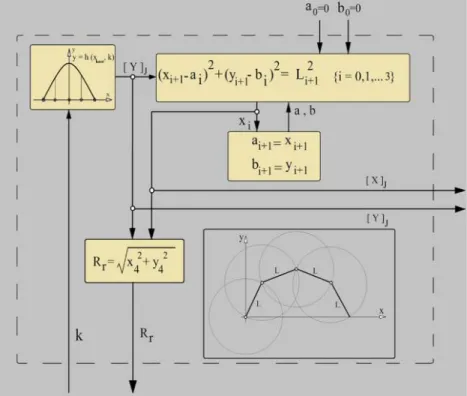
Figure 5 The computational geometric algorithm designed to calculate the Cartesian position of the joints and the real radial distance Rr

based on input k together with the knot vector Xknot. Xknotis vector of five points evenly distributed between the two roots of the parabola

(it is illustrated in the top-left box of this figure)

Figure 6 The control algorithm designed to regulate the k value to reach eⴝ Ea

Table I RMSE, computation time and minimum acceptable error as

result of simulation with optimal step size and optimal MAE

Trajectory Optimal␧ Optimal MAE (m) RMSE (m) CTSP (ms) Polynomial 3.75⫻ 10⫺4 _{4.50⫻ 10}⫺4 _{0.0133 5.06⫾ 0.12} Circular 4.69⫻ 10⫺4 _{1.00⫻ 10}⫺4 _{0.0012 18.02⫾ 0.68} P-shape 5.4_{⫻ 10}⫺4 _{4.00⫻ 10}⫺4 _{0.0019 4.93⫾ 0.41} Elliptic 4.06_{⫻ 10}⫺4 _{3.20⫻ 10}⫺4 _{0.0019 15.97⫾ 0.52} Oval spring 7.5⫻ 10⫺4 1.47⫻ 10⫺4 0.00006 19.53⫾ 0.13

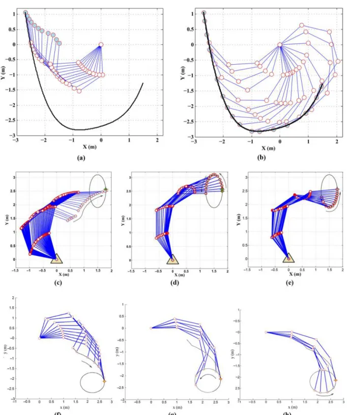
Figure 7 The predicted postures of the redundant robot. Black line represents the path of the end-effector, red square corresponds to the position which is selected based on random values of k and␭.

Geometric algorithm) to generate motion for redundant robotic manipulators. The main advantage of this algorithm is to be Jacobian-free: singular/near singular points will not represent a problem anymore. First, the redundant mechanism is modeled as a system with two DOFs considering a prismatic and revolute

joint regardless of the numbers of DOFs. The geometry of the robot’s workspace is formulated in polar coordination using linear and rotational displacement. A joint synergy is designed in a way that forms the configuration of robot as a parabola. So that, the linear distance could be regulated by adjusting the curvature. Figure 8 The predicted postures for three paths

In the second section, the unified framework used for the motion planning is introduced. Third section describes a geometric algorithm which consists of two separate subparts: “control algorithm” and “geometry of system”. As results, four sample end-effector trajectories are designed, and their relevant joint profiles are generated using the proposed geometric algorithm. Then the three-dimensional extension of this approach will be presented.

2. Unified motion planning framework

The simplified 2-DOF mechanism is presented as the model of a planar redundant robot (q1 and q2are the DOFs shown in

Figure 1(b)). The algorithm presented inFigure 2uses xTand yT

as time-dependent variables of Cartesian position of end effector and then it transforms these variables to polar coordination Rd

and␭d. These parameters are equivalents of q1and q2represented inFigure 2. Actually, Rd and␭d are distance and angle of the

target point respect to the base of robot, respectively. Then, the

geometrical algorithm calculates the Cartesian positions of joints.

Joint positions are a set of the postures of robot to reach the target point. The关X兴jand 关Y兴j are vectors of joint positions defined

according to equation (1). The xi and yi are horizontal and

vertical position of ith_{joint, respectively.}

The kinematical transformation translates the joint variable from workspace into joints space. Finally,␭ is added to the angle of the first joint to locate the end effector at the target point position. The joint angles are regulated to adjust radial distance Rdand after that the first joint angle is also adjusted

by adding␭:

关X兴j ⫽ 关x1x2x3. . .xn兴;关Y兴j ⫽ 关y1y2y3. . .yn兴 (1)

2.1 Geometric algorithm

The central part of this paper deals with the geometric-based computational algorithm which calculates the Cartesian positions of joints. The main idea of the proposed algorithm is to control the robot posture to reach the target point.

Let us assume that a planar redundant robot is configured in a parabolic posture. Given k as the coefficient of the formulation of this curve and R as the distance between its roots, an inverse relation between k and R can be found with respect to the Figure 3. In fact, this figure shows that increasing coefficient k causes the reduction of R. The main idea is to regulate the coefficient k to reach to desired radial distance R. The error signal e is computed as difference between the real and the desired distances, Rr and Rd,

respectively.

The control algorithm uses the e to regulate the control variable k to set the end effector on the target point. Then this value is used by a computational algorithm to calculate the vertical and horizontal position of joints. The closed loop system is designed to regulate the posture of robot to reach to desire distance Rd(Figure 4).

2.2 Geometry of system

A second-order polynomial function h共xknot, k兲 is implemented to calculate the vertical position of the joints. In fact, the k value would determine the curvature of the parabola, while the knot vector of xknotprovides preliminary horizontal position. Later on, the resulted vertical position of joints 关Y兴J is integrated in geometric model of a redundant planar robot (illustrated in bottom right box of Figure 5) to calculate horizontal position of joints 关X兴J. This geometry takes Figure 9 The simulation results of P-shape trajectory tracking (4 DOFs). The predicted postures are shown in (a)–(e)

advantage of the equation of a circle to describe the locus of the tip of the each link. To understand it better, let us consider the joint as located at the center of a circle, so the position of tip of the link could be described by the equation of circle with diameter as long as length of the link.

In equation (2), xi⫹1and yi⫹1are the horizontal and vertical position of the end of the共i ⫹ 1兲th_{link, respectively, a}

iand bi are the horizontal and vertical position of joint of共i ⫹ 1兲th_link, respectively. The Li⫹1 is the length of the共i ⫹ 1兲th link. By using this equation and considering a0⫽ 0, b0⫽ 0 (as the position of the first joint) and using y1which is calculated from “control algorithm” section, x1 is calculated. Based on a recursive method shown in Figure 5, the x2, x3, x4 are obtained.Figure 5also illustrates this recursive algorithm to calculate the vertical and horizontal position of joints based on a given k value: (xi⫹ 1 ⫺ ai) 2 _{⫹ (y} i⫹ 1 ⫺ bi) 2 _{⫽ L} i⫹ 12 (2) 2.3 Control algorithm

Figure 6 depicts how the control algorithm computes the k value for a given error e. For a negative error, the k initiates with a value greater than 1, and for the positive error, k initiates with the value between 0 and 1.␧ denotes step size used to increase or decrease the k value and the i is counter variable of the loop. Eais the acceptable error: it has a positive

value defined inTable I.

3. Simulation of planar task

The foregoing algorithm is used for point-to-point motion planning, in fact, any given trajectory must be divided into control points: the approach aims to predict the motion between every two control points. A 4-DOF planar robot manipulator is considered for point-to-point motion planning task. Each of the four links is 1-m length. Three different sample trajectories are used for validation purposes. For each

Figure 10 End-effector tracking error during polynomial, circular,P-shape and elliptic trajectory tracking (top to bottom)

trajectory, the motion initiates from a random position indicated by random values of k and␭, and it continues till reaching the starting point. The end effector starts motion from initial point and locates at final position in times t⫽ 0 and t⫽ T, respectively.

Figure 7 shows the predicted path and postures from a random initial position to the starting point and from the starting point to the final position indicated by red squares and red stars, respectively. The random initial points are generated using the angle␭ and the desired radial distance Rdobtained

from parameter k (Figure 3).

The algorithm generates the end-effector path and joints position of the robot to move the end effector between the given initial and final points. Three continuous trajectories have been simulated and tested to show the algorithm performance for open or closed paths.

The first sample trajectory is represented by a fourth-order polynomial curve for interval x␧关 ⫺ 2.4, 1.5兴 defined by (3). The considered path of the end effector is digitized to control points and then the algorithm is integrated to predict the path and postures between every two points. Figure 7 shows predicted postures of the 4-DOF redundant robot manipulator. Four sample trajectories were selected to validate the control algorithm: polynomial, elliptic, circular and “P”-shape trajectory. Trajectory (1) (top row plots in

Figure 8) was computed as follows:

y⫽ ⫺2.7 ⫹ 0.27x ⫹ 1.5x2⫹ 0.07x3⫹ 0.09x4 ₍₃₎ The initial position is chosen randomly based on random k and␭ values as mentioned before. Top row plots inFigure 8

illustrate the predicted motion of the robot following polynomial trajectory. The elliptic trajectory (middle row plots in Figure 8) was computed according to equation (4). It represents a circle with 0.5-m radius whose center is located at (2.2 m,⫺2.2 m):

(x⫺ 1.5)2

0.09 ⫹

(y⫺ 2.5)2

0.36 ⫽ 1 (4)

The circular trajectory (bottom row plots in Figure 8) corresponds to a circular path computed according to equation (5) whose radius is 0.5 m and center located at (2.2 m,⫺2.2 m):

(x⫺ 2.2)2_{⫹ (y ⫹ 2.2)}2_{⫽ 0.25 (5)} The trajectory presented inFigure 9corresponds to the shape of the letter “P”. The trajectory consists of straight lines (B and E), curves (C and D) and Section A positioning on start point.

Figure 10shows the tracking error for the mentioned paths. The error is calculated as horizontal and vertical deviation of the predicted position (xp, yp) from the desired trajectory (xd, yd) according to equation (6):

Error⫽

兹

d⫺ yp)

2 ₍₆₎

Here we introduce the “Optimal Point Analysis” method which is used to find optimal value for the critical parameters of the algorithm. These parameters are “Step Size” and

“Acceptable Error” which represent the performance indicators for algorithm’s speed and accuracy, respectively. As these factors have opposite trends, the maximum efficiency is usually achieved just by finding a trade-off between speed and accuracy. Accordingly, we define the algorithm’s optimal point as an amount of step size and acceptable error which leads to achieve highest computational speed and accuracy at the same time. To reach this goal, we applied the algorithm to analyze the optimal point illustrated byFigure 11.

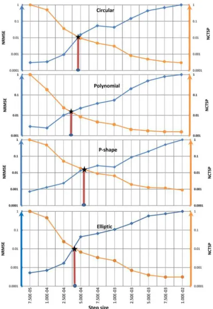
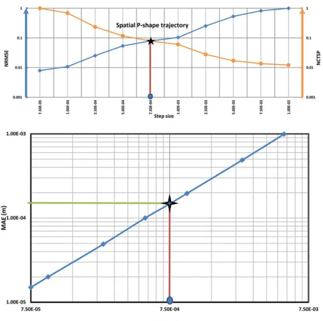
The calculated normalized root mean square error (NRMSE) and normalized computational time for single point (NCTSP) are plotted against step size ␧ (for the ten values) and four trajectories (Figure 12). As expected, decreasing the resolution of the algorithm (by increasing step size) leads to the decreasing accuracy and increasing computation speed. Hence, the optimal algorithm resolution␧ is obtained through making a trade-off between NRMSE and NCTSP. Accordingly, the intersection of these two graphs gives optimal␧ which, by using the minimum acceptable error (MAE) and ␧ diagram (Figure 13), will also give⫺the optimal MAE. The optimal values of MAE and␧ used to generate the motion for the four trajectories are shown inTable I.

4. Spatial motion planning algorithm

In this section, we discuss how to use the proposed algorithm to control a 7-DOF anthropomorphic robotic manipulator during a three-dimensional task. The presented motion planning approach creates a single 2D arm flexion which has effect on the planar motion of the end effector. To create a

Figure 11 Optimal point analysis flowchart

Figure 12 Normalized RMSE (NRMSE) and normalized computational time for single point (NCTSP) on primary and secondary vertical axes respectively, step size on the horizontal axis. The intersection points shown by stars indicate the optimal step size

Figure 13 MAE plotted versus algorithm step size

spatial positioning (for end effector), we need more than one planar motion so that we propose two separate joint synergies in which each one creates a single planar motion. Consequently, by the combination of two planar motions, we would have a spatial motion of the end effector. Each synergy is controlled by the planar motion planning algorithm presented in the previous section.

The anatomy of human arm movements is described by three pairs of terms: supination/pronation, felction/extension and abduction/adduction. In this part, we present a pair of synergies which allows the anthropomorphic robotic manipulator to mimic the first two movements of the human arm. In particular, the first synergy is in charge of controlling the arm bending in the u-w plane (Figure 14 (b)) by means of control over even joints which resemble human arm flexion/ extension. The second synergy is used to create an axial torsion among whole arm in u-v plane (Figure 14 (c)) via controlling the odd joints. This motion look likes human arm supination/pronation (Figure 14 (c)). Consequently, the combination of these two synergies will lead to achieve a generic spatial positioning of the end effector (Figure 14 (d)). A three-dimensional motion is achieved by combining two 2D motions: the following section describes the control of the three-dimensional motion.

4.2 Modeling and motion control

To control the end-effector position, a cylindrical coordination is considered (Figure 15 (b)). The height of the cylinder is

controlled by a second joint, while the alpha angle would be adjusted by the first joint.

The length r is regulated by the combination of two synergies. The r value is regulated by changing the k value of synergies and then the height of the target point is compared with the height of the end effector. After this, the error angle for the second joint is calculated (to compensate the distance between the height of end effector and the height of the target point) and then the error angle of the first joint is defined as the difference between the alpha angle of the target point and the end effector. In each iteration, by adding these two

Figure 14 The top row shows an anthropomorphic 7DOFs robotic manipulator controlled by joint synergies and lower row illustrates the equivalent of the whole arm motion

Figure 15 The 3DOFs cylindrical model. XEis the position of the

end-effector described by_{␣, h and r. The control variables ␣ and h} are regulated respectively by the angles of first and second joint (␪1

and_␪2) while the third control variable (r) is adjusted by rest of the

joints (␪3-␪7)

compensation terms to the predicted joint angle, the end effector may be aligned across the target point.

The entire control model consists of a controller and a feedback/compensatory compartments (Figure 16). The controller section includes a planar motion planning algorithm which is cascaded with two set of synergies. The planar motion planning block presented in Figure 16 is the same as the geometric algorithm shown in Figure 4 where the inner feedback is replaced by an external feedback loop. It generates joint angles for a planar 3-DOF model then the synergies feed the angles to odd and even joints (Figure 17). Considering red dots on the top corner of bar in Figure 14 (b and c), intuitively, we can see that the bending has a greater contribution in red dot displacement than torsion. We can apply the same observation to the robotic arm and conclude that the joints which create bending have a higher contribution in the end-effector motion. Hence, the even joints receive a greater coefficient than odd joints.

The feedback/compensatory section is designed to correct the first and second joint angle to regulate control variables␣ and h (presented inFigure 15) and also provides a feedback for the controller section. The feedback block also provides the R⬙r value which represents the real position of the end effector when it is aligned with target point. This value is implemented to calculate the position error of the end effector which is the input of planar motion planning block. The compensatory part receives the predicted joint angles from the output of synergies and calculates the required angles for the first and second joint to locate end effector at the height hd and angle␣d(Figure 18, top).

To achieve this goal, we first assume that the joints are fixed except of the second joint. In this situation, the trajectory of the end effector is represented by a circle in the xz plane (blue circle inFigure 18 (b)). Hence, by regulating the␪2, the height of the end effector would vary in xz plane. Considering the block diagram in Figure 18, it first solves

the forward kinematic to obtain the current position of the end effector Xrand then it exploits equations (7)-(11) for calculating the angles ␤d and ␤r. Finally, by adding the differential value⌬␤ to the current angle of the second joint, the end effector is located at the desired height hd. The next step is aimed to regulating the angle␪1to relocate the end effector from␣’rto␣dwhere it would align with the target point. The new position of the end effector X’ris obtained by solving the forward kinematics for the current joint angles (considering the updated value for second joint␪2). Assuming that all joints except for the first are fixed, the trajectory of the end effector is represented by the circle (violet line inFigure16 (c)). To be aligned with the target point Xd, it just required to reach the green point which is achieved by rotating the first joint as⌬␣. The new position of the end effector X⬙ris closer to the target point. The next step is to achieve the target point by increasing/decreasing the length of AX¡ vector which is carried out by ther controller: AXr ¡ ⫽ OX¡ ⫺ OAr ¡ (7) AXd ¡ ⫽ OX¡ ⫺ OAd ¡ (8) hr⫽ zAX¡_r (9) hd⫽ zAX d ¡ ₍₁₀₎ Rxz⫽

兹

4.3 Spatial motion simulation results

We designed an oval spring-form trajectory defined by (12) for end effector and then analyzed the optimal point of the algorithm for this trajectory (Figure 19).Figure 20illustrates Figure 16 Block-diagram representation of the spatial motion planning algorithm. It consisted of controller (on top) and a feedback/

compensatory part on bottom

Figure 17 Scheme of planar motion planning algorithm presented in figure 16. The parameters q1, q2and q3are the predicted angles and e

is the error signal of vector R (e_{ⴝ R}dⴚ Rrⴖ)

the predicted joint profiles for the given trajectory. In this figure, four polynomial functions (of order 10) are fitted to the predicted joint angles to provide an analytical formulation for joint profiles. Equation (13) represents the analytical formula of whole joint profiles:

再

兺

To explore the effect of the synergy coefficient on positioning the end effector, we ran the program for a range of values for second synergy coefficient Kh僆 关0.1, 0.9兴.

Meanwhile, the coefficient of first synergy is kept equal to 1

to assure that this synergy has a higher coefficient value (because it feeds the even joints). The top graph inFigure 21shows the RMSE values of each run plotted for various

Kh values; bottom graph shows the Kh value with highest

accuracy (lowest RMSE). The top graph in Figure 21

depicts the facts that by increasing the contribution of second synergy, the accuracy of algorithm predictions will decrease. Accordingly and also by considering Figure 14 (c), the torsion would endangered the positioning accuracy of end effector. The lower graph shows the synergy coefficients which results in minimum RMSE.

A 3D R letter-shape trajectory is designed to show that the algorithm can work even in near singular positions. For this purpose, we plotted the manipulability measure (14) – which stands for Jacobian determinant of redundant robotic arms – for this trajectory (Figure 22). The graph shows that the algorithm works well in near singular points, and the image c on top proves this fact by illustrating a fully stretched posture. Figure 18 The top part shows the block⬙Compensation terms for first and second joints⬙ presented inFigure 16. The algorithm receives joint angles_{⌰ and target position X}das inputs and calculates the angles of first and second joints

In Figure 22, the position error of the end effector is also plotted together with manipulability index to present the behavior of end effector among trajectory and specifically in near singular point:

w ⫽ 兹det(J共⌰兲J(⌰)T_{) (14)}

5. Discussion and conclusion

The biomimetic motion planning approach is presented in two episodes: the first was a planar motion planning approach and, second, integration in a 3D motion generation algorithm. The prior takes advantage of a 2-DOF simplified non-redundant model of manipulator which is implemented in a feedback control loop (Figure 4) to control the position of end effector in a plane. In fact, the kinematic redundancy provides a potential capability to create various robot structure

morphology, so the core idea is to exploit the meaningful morphology which locates robot end effector in a given position.

In the later episode, we took inspiration from the biological concept of postural synergies to introduce two joint groups/ synergies that each one creates, i.e. an independent 2D morphology. The human arm movements are considered to design and combine the postural synergies in a way that each synergy follows a anatomical motion. Consequently, the superposition of these two postural synergies would create a curvature which leads to a 3D positioning of end effector. Since each synergy is controlled by an independent parabola, so, just two variables (the curvature values of parabolas) are required for controlling all of the 7 DOFs. In other words, applying the joint synergy concept causes a simplification in controlling the redundant manipulator.

Figure 19 Optimal point analysis for 3D oval-shape trajectory. The optimal step size and optimal MAE would be 7.5⫻ 10– 4_{and 1.47⫻ 10}– 4 respectively

The spatial motion planning algorithm was used to predict the joint angles for a 7-DOF anthropomorphic robotic manipulator following a 3D oval spring. The resulted joint angles presented in Figure 20 illustrate the continuity and

smoothness of joint profiles. Because of these two main features, we were able to fit a set of polynomial equation of order 10 over the predicted joint angles which result in an analytical formulation for joint profiles (Table II). Figure 20 Joint analytical angle profiles plotted for 3D oval-shaped trajectory

Figure 21 Top graph: RMSE plotted for tracking 3D oval-shape trajectory with different values of synergy coefficient Kh. Lower graph: zoom-in

for area Kh僆 [0.1, 0.4] which depicts Khvalue with minimum RMSE value (Kh⫽ 0.2)

Furthermore, by designing time function T共t兲 in equation (14), we can manage the velocity of predicted motion. It is worth mentioning that the considered mechanism in planar motion planning, given inFigure 17, has three DOFs with equal length of linkages and it follows a parabolic curve, so, inevitably, the predicted angles for second and third joints may have been the same. Accordingly, the profiles of third and fourth joints have the same trend of fifth, sixth and seventh joints because those are commanded by q2and q3(Figure 17). We designed a more complex trajectory for end effector to analyze the algorithm in terms of singularity and tracking

behavior. The path is designed as “R” letter shaped to embed both direct lines (vertical and diagonal) and curves and it is positioned as far as possible from robot (in a way that a part of trace would be on the boundary of robot’s workspace). The manipulability measure in Figure 22 decreases as end effector’s distance (from the origin) increases and in the point c has its minimum value. The c is a point close to singularity, as the value of manipulability measure is almost zero which intuitively can be seen in snapshot c (whole joints are aligned). The singularity at the point c also causes a change in sign of end effector’s position error.

Figure 22 Upper graph: robot configurations during tracking an “R” letter-shaped trajectory: middle graph: position error of the end-effector; lower graph: equivalent manipulability measure during the trajectory tracking

Table II. Values of polynomial coefficients for joint angle profiles

Joint no. P0 P1 P2 P3 P4 P5 P6 P7 P8 P9

1 4.93E-21 _⫺6.49E-18 3.55E-15 _⫺1.04E-12 1.79E-10 _⫺1.79E-08 1.07E-06 _⫺6.00E-05 0.003425872 0.308168582

2 _⫺9.87E-21 1.31E-17 _⫺7.20E-15 2.14E-12 _⫺3.74E-10 3.99E-08 _⫺2.51E-06 6.86E-05 0.000495263 0.144486011

3, 5, 7 1.11E-23 2.79E-20 _⫺4.11E-17 2.05E-14 _⫺5.21E-12 7.67E-10 _⫺7.89E-08 9.15E-06 _{⫺0.000967951 ⫺0.016354665}

4, 6 5.53E-23 1.40E-19 ⫺2.05E-16 1.03E-13 ⫺2.60E-11 3.83E-09 ⫺3.94E-07 4.58E-05 ⫺0.004839756 ⫺0.081773326

The simulation results (Figures 8and9for planar robot and

Figure 20for spatial manipulator) illustrate that the posture of robot varies continuously with no self-collision, while the end effector strictly follows the predefined planar trajectory. Comparison of the resulting error magnitude (i.e. millimeter) with the robot size (4 meters) convincingly demonstrates that the position error is rather negligible (Figure 10) for planar motion planning. The values of RMSE show the algorithm’s stability (Table I). The low computational time for single point (CTSP) values also show that the algorithm can be used for a real-time motion planning (Table I).

The algorithm will not be endangered by kinematic singularities, as it is not using the Jacobian-based solutions for motion planning. The analytical angle–time equations of joints are scalable which allowed us to design a desired velocity for joints to achieve desired dynamic at end-effector level. As the robot’s configuration follows a parabolic curve, the self-collision will not happen ever. In summary, singularity free, low computational burden, self-collision avoidance, joint profiles scalability and algorithm stability are the main advantages of the presented approach.

References

Abedi, P. and Leylavi Shoushtari, A. (2012), “Modelling and simulation of human-like movements for humanoid robots”, Proceedings of 9th International Conference on

Informatics in Control, Automation and Robotics (ICINCO) CITEPRESS, Rome, Italy, pp. 342-346.

Artemiadis, P.K., Katsiaris, P.T. and Kyriakopoulos, K.J. (2010), “A biomimetic approach to inverse kinematics for a redundant robot arm”, Autonomous Robots, Vol. 29 Nos 3/4, pp. 293-308.

Asuni, G., Leoni, F., Guglielmelli, E., Starita, A. and Dario, P. (2003), “A neuro-controller for robotic manipulators based on biologically inspired visuo-motor co-ordination neural models”, Proceedings of First International IEEE EMBS Conference on Neural Engineering, Capri Island, Italy, pp. 450-453.

Asuni, G., Teti, G., Laschi, C., Guglielmelli, E. and Dario, P. (2006), “Extension to end-effector position and orientation control of a learning-based neurocontroller for a humanoid arm”, Proceedings of the 2006 IEEE/RSJ International

Conference on Intelligent Robots and Systems, Beijing, China,

pp. 4151-4156.

Caggiano, V., De Santis, A., Siciliano, B. and Chianese, A. (2006), “A biomimetic approach to mobility distribution for a human-like redundant arm”, Proceedings of the IEEE/

RAS-EMBS International Conference on Biomedical Robotics and Biomechatronics, Pisa, Italy, pp. 393-398.

Chang, P.H. (1987), “A closed-form solution for inverse kinematics of robot manipulators with redundancy”, IEEE

Transactions on Robotics and Automation, Vol. 3 No. 5,

pp. 393-403.

Chen, T.H., Cheng, F.T., Sun, Y.Y. and Hung, M.H. (1994), “Torque optimization schemes for kinematically redundant manipulators”, Journal of Robotic Systems, Vol. 11 No. 4, pp. 257-269.

Chiaverini, S. (1997), “Singularity-robust task-priority redundancy resolution for real-time kinematic control of

robot manipulators”, IEEE Transactions on Robotics and

Automation, Vol. 13 No. 3, pp. 398-410.

Cruse, H., Wischmeyer, E., Bruser, M., Brockfeld, P. and Dress, A. (1990), “On the cost functions for the control of the human arm movement”, Biological Cybernetics, Vol. 62 No. 6, pp. 519-528.

Guglielmelli, E., Asuni, G., Leoni, F., Starita, A. and Dario, P. (2006), “Neurocontroller for Robot arms based on biologically inspired visuomotor coordination neural models”, in Akay, M. (Ed.), Handbook of Neural Engineering, John Wiley & Sons, Hoboken, NJ, pp. 433-448.

Hollerbach, J.M. and Suh, K. (1987), “Redundancy resolution of manipulators through torque optimization”,

IEEE Journal on Robotics and Automation, Vol. 3 No. 4,

pp. 308-316.

Khatib, O., Demircan, E., De sapio, V., Sentis, L., Besier, T. and Delp, S. (2009), “Robotics-based synthesis of human motion”, Journal of Physiology-Paris, Vol. 103 Nos 3/5, pp. 211-219.

Kim, C., Kim, D. and Oh, Y. (2005), “Solving an inverse kinematics problem for a humanoid robot’s imitation of human motions using optimization”, in Proceedings of the

Second International Conference on Informatics in Control, Automation and Robotics, ISBN 972-8865-30-9, pp. 85-92.

DOI: 10.5220/0001180100850092.

Leylavi Shoushtari, A. (2013), “What strategy central nervous

system uses to perform movement balanced?

Biomechatronical simulation of human lifting”, Applied

Bionics and Biomechanics, Vol. 10 Nos 2/3, pp. 113-124.

Maciejewski, A.A. and Klein, C.A. (1985), “Obstacle avoidance for kinematically redundant manipulators in dynamically varying environments”, International Journal of

Robotic Research, Vol. 4 No. 3, pp. 109-117.

Nakamura, Y., Hanafusa, H. and Yoshikawa, T. (1987), “Task-priority based redundancy control of robot manipulators”, International Journal of Robotic Research, Vol. 6 No. 2, pp. 3-15.

Palli, G., Melchiorri, C., Vassura, G., Scarcia, U., Moriello, L., Berselli, G. and Siciliano, B. (2014), “The DEXMART hand: mechatronic design and experimental evaluation of synergy-based control for human-like grasping”, The International Journal of Robotics Research, Vol. 33 No. 5, pp. 799-824.

Pollard, N.S., Hodgins, J.K., Riley, M.J. and Atkeson, C.G. (2002), “Adapting human motion for the control of a humanoid robot”, Proceedings of IEEE International Conference on Robotics and Automation, Vol. 2, pp. 1390-1397.

Potkonjak, V., Popovic, M., Lazarevic, M. and Sinanovic, J. (1998), “Redundancy problem in writing: from human to anthropomorphic robot arm”, IEEE Transaction on Systems,

Man and Cybernetics, Part B, Vol. 28 No. 6, pp. 790-805.

Qiao, H., Li, C., Yin, P., Wu, W. and Liu, Z.Y. (2015), “Human-inspired motion model of upper-limb with fast response and learning ability: a promising direction for robot system and control”, Assembly Automation, Vol. 36 No. 1.

Ramos, M.C. and Koivo, A.J. (2002), “Fuzzy logic based optimization for redundant manipulators”, IEEE Transactions on Fuzzy Systems, Vol. 10 No. 4, pp. 498-509.

Santello, M., Flanders, M. and Soechting, J.F. (1998), “Postural hand synergies for tool use”, The Journal of

Neuroscience, Vol. 18 No. 23, pp. 10105-10115.

Seraji, H. (1989), “Configuration control of redundant manipulators: theory and implementation”, IEEE Transactions on Robotics and Automation, Autom., Vol. 5

No. 4, pp. 472-490.

Siciliano, B. (1990), “Kinematic control of redundant robot manipulators: a tutorial”, Journal of Intelligent and Robotic

Systems, Vol. 3 No. 3, pp. 201-212.

Suarez, R., Rosell, J. and Garcia, N. (2015), “Using synergies in dual-arm manipulation tasks”, Proceedings of IEEE

International Conference on Robotics and Automation (ICRA), Seattle, WA, pp. 5655-5661.

Torres-Oviedo, G., Macpherson, J.M. and Ting, L.H. (2006), “Muscle synergy organization is robust across a variety of postural perturbations”, Journal of Neurophysiology, Vol. 96 No. 3, pp. 1530-1546.

Wang, J. (1997), “Recurrent neural networks for computing pseudo-inverses of rank-deficient matrices”,

Siam Journal on Scientific Computing, Vol. 18 No. 5,

pp. 1479-1493.

Whitney, D.E. (1969), “Resolved motion rate control of manipulators and human prostheses”, IEEE Transactions on

Man-Machine Systems, Vol. 10 No. 2, pp. 47-53.

Whitney, D.E. (1972), “The mathematics of coordinated control of prosthetic arms and manipulators”, Journal of

Dynamic Systems Measurement and Control, Vol. 94 No. 4,

pp. 303-309.

Xia, Y. (1966), “A new neural network for solving linear programming problems and its application”, IEEE Transactions on Neural Networks, Vol. 7 No. 2, pp. 525-529.

Yoshikawa, T. (1985), “Manipulability of robotic mechanisms”, International Journal of Robotics Research, Vol. 4 No. 2, pp. 3-9.

Corresponding author

Ali Leylavi Shoushtari can be contacted at:

a.leylavishoushtari@sssup.it

For instructions on how to order reprints of this article, please visit our website:

www.emeraldgrouppublishing.com/licensing/reprints.htm

Or contact us for further details:permissions@emeraldinsight.com