Analysis of the penumbra formation in sunspots

UNIVERSIT `A DEGLI STUDI DI CATANIA Dipartimento di Fisica e Astronomia

Dottorato di Ricerca in Fisica XXX Ciclo

Mariarita Murabito

ANALYSIS OF THE PENUMBRA FORMATION IN SUNSPOTS

Tesi di Dottorato

Coordinatore: Prof. V. Bellini

Tutor: Chiar.ma Prof.ssa F. Zuccarello Cotutors: Dott. P. Romano

Contents

Abstract 4

1 Introduction 7

1.1 Solar Active Region morphology and evolution . . 7

1.1.1 Mount Wilson classification . . . 8

1.1.2 Evolution of ARs . . . 10

2 Sunspots: observations and models 15 2.1 Sunspot physical parameters . . . 16

2.1.1 Fine structure of sunspots . . . 17

2.2 Evershed flow . . . 26

2.3 Penumbra formation . . . 30

2.4 Simulations of penumbra formation . . . 39

3 High resolution observations 42 3.1 Ground-based observations: Interferometric BIdimensional Spectropolarimeter/DST . . . 43

3.2 Space-based observations:

SDO . . . 46 3.3 Spectro-polarimetry and data inversion technique 51 3.3.1 The SIR code . . . 54 3.3.2 Azimuth ambiguity . . . 55 4 Penumbra formation in a region without flux

emer-gence 57

4.1 Observations . . . 58 4.2 Analysis . . . 59 4.3 Results . . . 62 5 Penumbra formation in a region of flux emergence 76 5.1 Observations and Analysis . . . 76 5.2 Results . . . 78 6 Penumbra formation in a sample of active regions 87 6.1 Observations and Analysis . . . 87 6.2 Location of the first penumbra sectors . . . 89 6.3 Evolution in the upper atmopheric layers . . . 101 6.4 Transition from inverse to classical Evershed flow 102

7 Discussion 108

7.1 A possible scenario for the penumbra formation . 108 7.2 Penumbra formation in the region between two

7.3 Settlement of the first penumbral filaments and their velocity field evolution . . . 111

Abstract

The formation of the penumbra in sunspots is a physical process which involve the coupling between the plasma and the magnetic field in different layers of the solar atmosphere. Its study requires long time series of observations carried out with high temporal, spatial, and spectral resolution. Moreover, due to few available datasets of this phase of the sunspot evolution, the physical pro-cesses at the base of the penumbra formation are still unclear. For this reason in this thesis I performed some observational analysis of the penumbra formation using high resolution data acquired during an observing campaign at the Richard B. Dunn Solar Telescope (NSO) and data taken by HMI onboard of SDO. Two main aspects have been investigated: the location of the stable settlement of the first penumbra filaments and the transition from inverse to classical Evershed flow.

Using the high resolution images I observed the first set-tlement of the penumbra filaments in the two polarities of AR NOOA 11490. Before the penumbra formation the pore of the preceding polarity exhibits an annular zone characterized by a

magnetic field greater than 1000 G, having an (upside down) ballerina skirt structure of the magnetic field. In this case, the penumbra starts to form in the side away from the opposite po-larity, in agreement with the observations of Schlichenmaier et al. (2010). On the other hand, using the same dataset, I showed that in the following polarity of the AR NOAA 11490 a stable penumbra forms in the area facing the opposite polarity, located below an AFS, i.e. in a flux emergence region.

Moreover, considering a sample of other six ARs observed by HMI, I found that there is no preferred location for the penumbra formation.

I interpreted the formation of the penumbra as due to the field lines of the magnetic canopy, already existing at a higher level of the solar atmosphere and overlying the pore, which sink down into the photosphere and below the solar surface. In fact, in this case there is a non-zero probability of finding near-horizontal field also in the region between the two main sunspots, as shown by the recent simulations of MacTaggart et al. (2016).

Concerning the transition from inverse to classical Evershed flow, in the preceding polarity of AR NOAA 11490 I found changes in the direction of the LOS velocity field during the formation of the first penumbral sector. In about 1-3 hours the LOS velocity became coherent with the Evershed flow pattern while the penumbra was completely formed. I also found obser-vational evidences of this transition in most of the pores of my

sample observed by HMI. Therefore, I proposed a new model to explain this transition in the velocity field, based on the presence of small U-loops, which are able to drive a siphon flow toward the pore, i.e., corresponding to the inverse Evershed flow, before the penumbra formation.

The thesis is organized as follows: in Chapter 1 I provide a brief introduction on the characteristics of the solar active re-gions. Chapter 2 describes the main features observed in solar sunspots with particular attention to the penumbra and its for-mation, taking into account both the observational and theoret-ical point of view. The used instruments, the data and their method of analysis have been described in Chapter 3. Chapters 4 and 5 report the analysis of the data concerning the preceding and following polarities of AR NOAA 11490, respectively. The study carried out using a sample of 6 ARs observed by HMI is reported in Chapter 6. A discussion containing a possible sce-nario for the penumbra formation and the transition from the inverse to the classical Evershed flow is reported in Chapter 7. The conclusions drawn from the results obtained in this thesis are reported in Chapter 8.

Chapter 1

Introduction

1.1

Solar Active Region morphology

and evolution

Active regions (ARs) are defined by the totality of observable phenomena from the photosphere to the corona as a result of the magnetic flux emerged from the convection zone, revealed by emissions over a wide range of wavelengths from radio to X-rays (van Driel-Gesztelyi & Green, 2015). The simplest ARs have a bipolar magnetic field configuration, but usually ARs may be built-up due to several bipoles emerging in close succession. Bipolar ARs are usually aligned in the east-west direction and for the Hale’s law they have opposite leading magnetic polarities on opposite hemisphere.

is manifested by the appearance of dark sunspots or pores1 _and

bright faculae representing concentrated and diffused magnetic fields, respectively. In the chromophere ARs are charcterized by the presence of arch filament systems (AFSs), filaments and bright regions called plages. The AFS are bundles of dark arches crossing the polarity inversion line (PILs) (Bruzek, 1968). The dark filamentary structures observed on the solar disk, called filaments, are due to dense and cold plasma suspended in the extremely hot corona. They are found above the PILs (Wang et al., 2017).

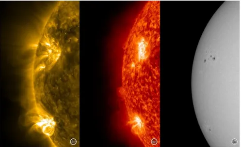
In the upper layers, i.e. transition region and corona, we observe that the magnetic opposite polarities are connected by bright, dense and hot loops. In figure 1.1 we show an example of ARs in photosphere, chromosphere and corona.

1.1.1

Mount Wilson classification

There are many classifications useful to describe the AR mor-phology. Here I report the Mount Wilson magnetic classification that describes the magnetic complexity of sunspot groups in pho-tosphere:

α - Unipolar sunspot group.

Figure 1.1: Active regions on the solar disk. From left to right: corona, chromophere and photosphere, respectively. SDO

β - A sunspot group with distinct and well separated positive and negative magnetic polarities.

β-γ - A bipolar sunspot group where the spots of opposite po-larity are not well separated.

γ - A sunspot group where the distribution of positive and neg-ative magnetic polarity is irregular.

δ - A sunspot group with complex magnetic configuration, con-sisting of opposite polarity umbrae within the same penum-bra.

1.1.2

Evolution of ARs

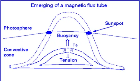
The magnetic flux tubes of the toroidal magnetic field gener-ated by the dynamo in the tachocline, are called Ω loops. During their rise from the convection zone into the upper layers of the solar atmosphere they are influenced by the Coriolis force, mag-netic tension, drag, plasma vortices and large-scale convective motions. Figure 1.2 shows a sketch of a flux tube that is rising from the convective zone.

When the magnetic flux tubes reach the photosphere, we ob-serve a nearly horizontal, upward-moving (≈ 1 kms−1) magnetic field with strength of 200-600 G. The individual flux elements at photospheric level move rapidly away from the emergence

Figure 1.2: Sketch of a magnetic flux tube rising from the con-vective zone. Bi indicates the magnetic field strength of the

magnetic flux tube, Pi and Pe are the gas pressures inside and outside the flux tube at the same height, respectively.

strength reaches values of kG. During this phase the granulation pattern is anomalous, i.e. the granules between the opposite po-larities become larger and elongated (Guglielmino et al., 2010). When the top of magnetic flux tubes emerges through the pho-tosphere, between the two opposite polarity flux concentrations (pores and spots) dark inter-granular lanes appear, being char-acterized by a lifetime of 10-30 minutes (van Driel-Gesztelyi & Green, 2015).

The bipolar magnetic field expands and bright plages appear. The configuration of the magnetic field starts to change, becom-ing a mixture of weak horizontal and more vertical field. On small scale, the magnetic field appears like serpentine, i.e. un-dulatory flux formed by an alternative series of small Ω and U-loops that cross the photosphere (Watanabe et al., 2008). Then an AFS appears in Hα images. Individual arches are short-lived (20-30 minutes), but the AFS exists as long as flux is emerg-ing (van Driel-Gesztelyi & Green, 2015). Right above the AFS we observe hot and brigth EUV and X-rays loops (Kawai et al., 1992; Malherbe et al., 1998). In this phase, usually, the pho-tospheric magnetic field reaches values of 2000-2500 G due to the convective collapse (Parker, 1978), where plasma drain out of the rising loops, increasing the strength of the magnetic field (Zwaan et al., 1985; Lites et al., 1998).

The same-polarity concentrations form pores that move to-wards each other and coalesce forming sunspots. The formation

of the penumbra around a pore is part of the flux emergence pro-cess. The emerging flux starts reconnecting with the surround-ing pre-existsurround-ing fields formsurround-ing new coronal magnetic connections. During the flux emergence process, we observe a high flare rate, but the flare number peaks when the sunspot area of the AR reaches its maximum.

When no new magnetic flux emerges anymore through the photosphere, the AR starts decaying. We observe, in this stage, small magnetic flux concentrations (MMFs) that move away from the sunspots. The first decaying signature in the sunspot evolution is the appearance of light bridges (LBs). Figure 3.1 shows the evolution of a sunspot and the formation of the LB. Usually, the flare activity decreases after a solar rotation, but the number of coronal mass ejections (CMEs) coming form the AR does not seem to decrease. In this phase, although the emission of chromospheric plages is still high, the magnetic field density decreases. Faint emission is revealed in the corona except for X-ray bright points related to the emergence and cancellation of smaller-scale flux (Sheeley, 1981; Schrijver & Zwaan, 2000; Har-vey & Zwaan, 1993). Finally, the enhanced network disappears and the AR loses its identity.

Figure 1.3: HMI/SDO images in the continuum of the preceding sunspot of NOAA AR 11263. The sequence shows the evolution of the sunspot umbra and the formation of a light bridge (Falco et al., 2016).

Chapter 2

Sunspots: observations

and models

Sunspots are the most prominent manifestation of magnetic flux emergence in the photosphere. The sunspot properties have been studied since their first observation (1610, Galileo and Steiner, Solanki (2003)) and their discover as locations of strong magnetic field (Hale, 1908). Our understanding of sunspots increases with the new facilities developed both for high resolution observations and MHD simulations.

2.1

Sunspot physical parameters

Sunspots are dark structures in the solar photophere. They are composed of an inner dark area, the umbra, and an outer less dark region with a filamentary structure: the penumbra. The magnetic field inhibites the convective flows, i.e. it supppresses the heat transport by convection, and for this reason sunspots are cooler than the surrounding solar photophere where the av-erage heat flux of 6.31×107 W/m2. Consequently the heat flux is reduced by 25% and 77% in the penumbra and the umbra, re-spectively (Rempel & Schlichenmaier, 2011). The effective tem-perature that corresponds to these heat fluxes are ∼ 5777 K, ∼ 5275 K and ∼ 4000 K for quiet Sun, umbra and penumbra, respectively.

Sunspots exhibit a broad size distribution, even if smaller sunspots are more common than larger ones. The size varies between 3500 km and 60000 km, from the smallest to the biggest ones (Solanki, 2003). Sunspots can have lifetimes of months or only hours. In general the sunspots lifetime depends on the sunspot size. The following rule was formulated for the first time by Waldmeier in 1955: A0 = W T , where A0is the mazimum size

of the spot, T the lifetime and W is a constant recently found to be equal to 1089±0.18 MSH day−1(MSH, Millionths of the Solar Hemiphere) according to Petrovay & van Driel-Gesztelyi (1997). The magnetic field is almost vertical in the central part of the

umbra, where it varies from 1800 G to 3700 G, while it decreases from the inner part to the outer edge of the penumbra, reaching values between 700-1000 G. In the penumbra the magnetic field is more inclined.

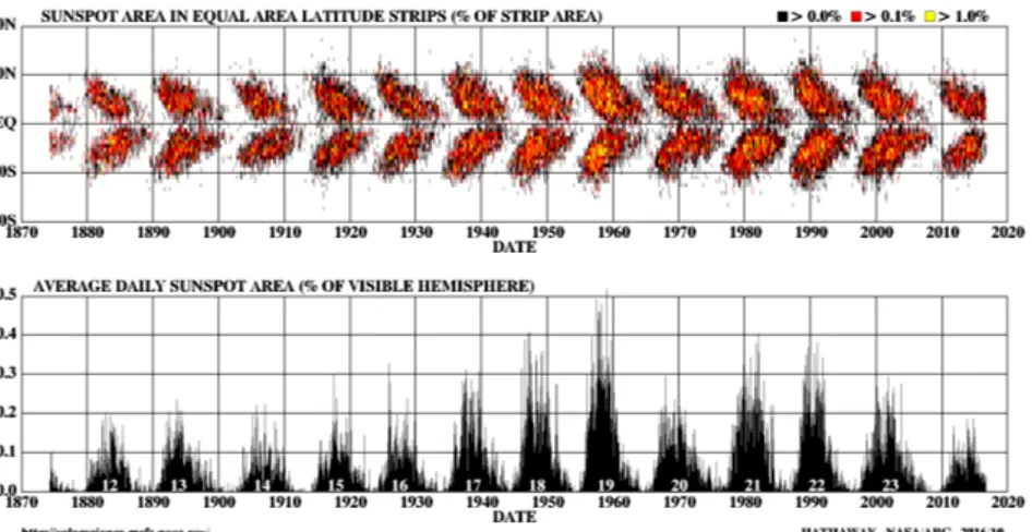
The number and the location of sunspots varies over the solar cycle. During the minimum it is possible that no sunspots are visible on the solar surface, while during the maximum it is usual to see 10 or more groups of sunspots. Usually they appear in a belt between +30◦ and −30◦ from the solar equator. Carrington in 1863 noticed that the sunspots location is not casual, but when the solar cycle starts, sunspots appear at high latitudes, sometimes up to 40◦ from the solar equator. During the cycle, sunspots appear at lower latitudes and at the end of the cycle they are very close to the equator. This behavior is well described by the so called ‘butterfly diagram’, shown in Figure 2.1.

2.1.1

Fine structure of sunspots

In the last 50 years space and ground-based observations have highlighed the dynamic and fine structure of the sunspots. De-spite the fact that sunspots are globally stable, a variety of small-scale features such as umbral dots (UDs), light bridges (LBs), bright and dark penumbral filaments, appear in the sunspots and evolve on a dynamic time scale.

Figure 2.1: Butterfly diagram for the years 1874-2016, NASA Umbral dots (UDs)

Umbral dots were observed for the first time in 1964 by Danielson (1964) as bright dot-like spots inside the umbra, with typical size less than 0.′′5 (see left panel of Figure 2.2). Although the UDs seem to be present in all sunspots, there is not a typical intensity value in photophere (Rempel & Schlichenmaier, 2011). From the observations it has been possible to estimate a temperature difference between them and the umbral background that ranges between 500 K and 1500 K at τ = 2/31 _{(Borrero & Ichimoto,}

2011). It is possible to distinguish two types of UDs: central umbral dots (CUDs), which appear close to the darkest region 1_{τ corresponds to the optical depth defined as dτ =κds, where κ is the}

Figure 2.2: Left panel: NOAA 10634 with LBs and UDs (Sobotka & Puschmann, 2009). Right panel: Complex sunspot crossed by several LBs (Solanki, 2003)

of the umbra and peripheral umbral dots (PUDs), which appear at the umbral and penumbral boundary (Borrero & Ichimoto, 2011).

Despite the study of the magnetic field in UDs has been really controversial, it seems that it is weaker than in the surroundings: it is 10% − 20% lower in CUDs and 5% − 10% lower in PUDs (Schmidt & Balthasar, 1994). The lower magnetic field inside UDs is a direct consequence of the convective motions. In fact, the magnetic field lines in the umbra are pushed by the convec-tive motions towards the edge of the convecconvec-tive cell, creating a region where the vertical component of the magnetic field vector is strongly reduced (Borrero & Ichimoto, 2011).

Light bridges (LBs)

Light bridges are bright and elongated features that cross the umbra. The right panel of Figure 2.2 shows an image of a com-plex sunspot with four LBs crossing the umbra.

LBs have a significantly lower magnetic field strength with respect to the umbra, with a reduction ranging from 200 to 1500 G (Leka, 1997). In addition to that, the magnetic field is more inclined, between 5◦ and 30◦ larger than in the umbra (Solanki, 2003).

Penumbral filaments

The penumbra is composed by dark and bright filaments and penumbral grains (see Figure 2.2). High spatial resolution ob-servations have shown small features in the penumbral filaments, which appear uniform at resolution worse than 1′′2. At high spa-tial resolution it can be seen that intensity, velocity field and magnetic field values indicate a filamentary structure (Rempel & Schlichenmaier, 2011). The filaments have a tipical width, ac-cording to Scharmer et al. (2002), of 0.′′2 - 0.′′25 in the continuum images. The dark and the bright filaments are characterized by a continuum intensity of ∼ 0.3 − 0.7 Icand ∼ 0.7 − 1.0 Ic,

respec-tively (Muller, 1973).

The magnetic field consists of two components: spines and intraspines. The magnetic field is stronger and more vertical

Figure 2.3: Sketch showing the interlocking-comb structure of the magnetic field in the filamentary penumbra of a sunspot (Thomas et al., 2002).

with respect to the solar surface in the spines, while the in-traspines are characterized by a magnetic field weaker and more horizontal (Borrero & Ichimoto, 2011). This magnetic field con-figuration is referred as ‘interlocking comb’ structure (Thomas & Weiss, 1992) or ‘uncombed penumbra’ (Solanki & Montavon, 1993) (Figure 2.3).

The magnetic field lines of the spines are connected with regions far from the sunspots, to form coronal loops over the active region, while the magnetic field lines of the intraspines turn back into the photosphere at the edge of the sunspot to form a canopy (Borrero & Ichimoto, 2011).

A possibile scenario that explains how the magnetic field lines return back into the solar surface at the edge of the penumbra

(intraspines) was formulated by Thomas et al. (2002). The key idea is that the outer part of the flux tubes are submerged by the downward pumping of the granular convection outside the sunspot, forming the low-laying horizontal flux tubes (Borrero & Ichimoto, 2011).

There are two models that try to explain the penumbra struc-ture:

• Embedded flux tube model: this empirical model, shown in Figure 2.4, was proposed by Solanki & Montavon (1993). In this case horizontal magnetic flux tubes (intraspines) are embedded in more vertical magnetic fields (spines). • Field free gap model: the penumbral bright filaments

repre-sent a protusion of non-magnetized, hot gas into the back-ground oblique magnetic fields of the penumbra. In Figure 2.5 a sketch of this model is shown. The left panel cor-responds to the model for an umbral dot, where the cusp is located below τ = 1. The surface around the gap is bright because of the radiative heat flux. The observed field strength is reduced due to the displacement of field lines by the gap. In the middle panel we see the configu-ration for a light bridge, where a wide gap would be seen as a field-free canal. Finally, the right panel illustrates the situation for the penumbral filament. The sketch is similar to that shown for the light bridge, but with an additional

Figure 2.4: Embedded flux tube model (Borrero & Ichimoto, 2011). The solid lines indicate the vertical magnetic field (spines) while the cylindrical structures the horizontal ones (intraspines). Dashed arrows indicate the direction of the flow.

horizontal field component (indicated by shading) along the filament.

The penumbra brightness is equal to 70% - 80% of the quiet Sun granulation. An important question is how the energy trans-port takes place to allow this brightness. The more efficient mechanism is surely the convection, but how does the convective motions in the presence of a strong (B≈ 1500 G) and horizon-tal (γ ≈40-80◦) magnetic field occur? The heat transport in the aforementioned feld-free gap model is very efficient because the convective motions are localized over the entire length of the bright filaments, with upflows at the center of the filaments and downflows at the filaments’ edges. This model predicts only

Figure 2.5: Sketch of the field-free gap model where gaps in a magnetic field near the solar surface (vertical cross-sections) are shown. Dashed lines indicate the continuum τ = 1 level. The two neighboring flux bundles spread out horizontally above the surface, forming a cusp at some height above τ = 1 (Spruit & Scharmer, 2006).

alternating upflows/downflows in the perpendicular direction to the filaments, azimuthally around the penumbra. For this reason this type of convection is referred to as azimuthal convection or overturning convection (see lower panel of Figure 2.6). A less effi-cient mechanism is represented by the hot rising flux-tube model, where the inner footpoints of the flux tube are characterized by upflows and the outer footpoints by downflows (Schlichenmaier, 2002). This type of convection is called radial convection, be-cause the convective flows occur along the penumbral filaments (see the upper panel in Figure 2.6)

Figure 2.6: Different patterns of convection in penumbral fila-ments. Upper panel: radial convection predicted by the hot ris-ing flux-tube model and the embedded flux-tube model. Bottom panel: azimuthal convection or overturning convection predicted by the field-free gap model (Borrero & Ichimoto, 2011).

2.2

Evershed flow

The Evershed flow is observed as a wavelength shift (red or blue) in the spectra of absorption lines in the penumbra (limb-side or disk-center). It was discovered by Evershed (1909) and can be explained by a nearly horizontal outflow in the penum-bra. It seems a stationary flow, observed at insufficient spatial resolution, with a typical velocity of ∼ 1-2 km s−1.

Since 1960s it was accepted that this flow is not spatially uni-form, but it is concentrated in narrow channels in the penumbra. Until 1990, two models were proposed to explain the fila-mentary structure of the penumbra and the Evershed flow. Both models assumed a nearly horizontal magnetic field in the penum-bra, but today this is not anymore supported by the observa-tional evidence that a significant fraction of sunspot’s vertical magnetic field is found in the penumbra (Borrero & Ichimoto, 2011). The discovery of the interlocking comb structure of the penumbra magnetic field solved the enigma on the Evershed flow. It seems in fact that the Evershed flow (middle panel of Figure 2.7) is correlated with regions where the magnetic field is hori-zontal (intraspines with γ ≈90◦, bottom panel of Figure 2.7) and weaker (upper panel of Figure 2.7).

The embedded flux-tube model (Solanki & Montavon, 1993) tries to explain the Evershed flow, assuming that it is confined in the horizontal magnetic flux tubes embedded in a more vertical

Figure 2.7: From top to bottom: Variation of the magnetic field strength B, line-of-sight velocity Vlos and inclination angle of

the magnetic fiel γ at τ = 1 (continuum) along an azimuthal cut around the limb-side penumbra. Dotted curves in each panel indicate the scattered light fraction obtained from the inversion algorithm (Borrero & Solanki, 2008).

background. Within this model, the siphon flow mechanism was proposed as the driver of the Evershed flow. The difference of gas pressure between the two footpoints of the flux tube is caused by a difference in the magnetic field strength. This difference of gas pressure drives the flow towards the footpoints with a higher field strength (Meyer & Schmidt, 1968; Thomas, 1988; Thomas & Montesinos, 1993).

pos-sesses a vertical component was found. In particular, the relatio-ship between the magnetic field vector and the vertical flow in the penumbra were clearly demonstrated by spectropolarimet-ric data. Figure 2.8 highlights this relationship for a spot near the disk center. The V maps, (see Chapter 5.1) at ±300 m˚A show two different patterns: in the -300 m˚A V map, small and elongated structures with the same polarity of the sunspot are visible in the inner penumbra, while in the +300 m˚A V map, patches of opposite polarity of the sunspot are seen in the mid and outer penumbra. These features are associated with upward (1 km s−1) and downward motions (∼4-7 km s−1), respectively (bottom panels in Figure 2.8) (Borrero & Ichimoto, 2011).

Taking into account the results concerning the velocity field and the magnetic field vector, it is possible to draw a picture of the penumbra as shown in Figure 2.9.

Even if the relationship between the Everhed flow and the intensity of the penumbra has been controversial, recent obser-vations demonstrate that the Evershed flow takes place in the bright filaments in the inner penumbra and in the dark filaments in the outer penumbra (Schlichenmaier et al., 2005; Bellot Rubio et al., 2006; Ichimoto et al., 2007).

One aspect however needs to be further investigated: the re-lationship between the penumbra formation and the estabilish-ment of the Evershed flow. Schlichenmaier et al. (2012) revealed, before the penumbra formation, a line of sight (LOS) velocity of

Figure 2.8: Upper and middle panels: Stokes V maps of a sunspot. Bottom panel: Doppler velocity (Borrero & Ichimoto, 2011).

Figure 2.9: Cartoon of the penumbral and Evershed flow struc-ture (Borrero & Ichimoto, 2011).

opposite direction with respect to that displayed by the typical Evershed flow at some azimuths. Figure 2.10 shows the contin-uum intensity and the LOS velocity evolution in the AR NOAA 11024 studied by Schlichenmaier et al. (2012), where the opposite Evershed flow is visible.

2.3

Penumbra formation

The presence of the penumbra distinguishes a mature sunspot from a pore. However, how and why the penumbra forms are still unknown, because their study requires long time series observa-tions (several hours) carried out with high temporal, spatial, and

Figure 2.10: Continuum intensity and LOS velocity maps of AR NOAA 11024 (Schlichenmaier et al., 2012)

spectral resolution (Thomas & Weiss, 2004).

Some recent studies have indeed provided some advancements in our knowledge of the formation of the penumbra. For in-stance, some authors assessed the presence of a critical value of some physical parameters above which penumbra formation takes place. Leka & Skumanich (1998) found that the magnetic field strength in a pore intensifies before penumbra starts to form. They estimated that the initial magnetic flux in a pore is around 2 × 1019 _{Mx, founding a threshold of 1-1.5 × 10}20_{Mx, above}

which the pore can develop a penumbra. From the analysis of spectropolarimetric data taken at the German Vacuum Tower Telescope (VTT), Rezaei et al. (2012) studied the formation of a sunspot penumbra in AR NOAA 11024. They found a magnetic field of the order of kilo-Gauss, inclined of 45◦ - 60◦ and extend-ing beyond the edges of the pore (as determined from intensity values). When the penumbra develops, the magnetic boundaries of the spot coincide well with the intensity contours of the pore. They found a critical magnetic field strength Bcrit ≤ 1.6 kG

and a critical inclination angle of the magnetic field γ ≥ 60◦ with respect to the normal to the photosphere, above which the penumbra begins to form.

In this context, Jurcak (2011) investigated nine stable sunspots using Hinode data and concluded that the umbra-penumbra (UP) boundary, traditionally defined by an intensity threshold, is also characterized by a critical value of the vertical component of the

magnetic field, Bstable

ver = 1860 (±190) G. Jurcak et al. (2015)

confirmed this result and found that, during the penumbra for-mation, the UP boundary migrates toward the umbra and Bver

increases. To explain this critical value of Bver, they propose

that there are two modes of magneto-convection. The penum-bral mode takes over in regions with Bver < Bstablever , while the

umbral mode prevails in regions with Bver > Bstablever .

In 2010 Schlichenmaier et al. acquired at the German VTT a 4.40 hr time series of continuum images of the Active Region NOAA 11024. They found that the penumbra formation occurs in sectors in the area away from the opposite polarity, and an individual penumbral sector forms on a time scale of about 30 minutes. In those areas, they found that filaments increase their radial extension, from 1′′ to 5′′ , becoming larger and more nu-merous. The filaments on the side facing the opposite polarity appeared to be not stable. This region was characterized by elongated granules that appeared and disappeared continuously. These elongated structures were associated with flux emergence and were also found in numerical simulations of Cheung et al. (2008) and Tortosa-Andreu & Moreno-Insertis (2009). These authors concluded that a stable penumbra cannot form in the region of flux emergence, because the strong dynamics owed to ongoing flux emergence prevent the settlement of the penumbral field.

were formed in a region on the side toward the opposite polar-ity of an AR. In this region a series of elongated granules were detected in association with an emerging flux region. However, they detected also cases where the flux emergence, even if ac-companied by a series of elongated granules, did not form the penumbra. They explained this double behavior with the pres-ence or abspres-ence of strong overlying canopy fields, concluding that both the amount of emerging flux and the existence of strong canopy field are important in the penumbra formation.

There are two main explanations for penumbra formation. Leka & Skumanich (1998) suggested that emerging, horizontal field lines could be trapped and form a penumbra rather than continuing to rise to higher layers, due to the presence of the overlying magnetic canopy in the emerging region.

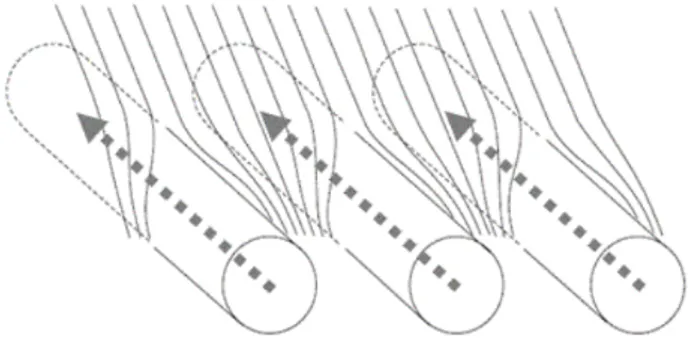
In contrast, Shimizu et al. (2012) and Romano et al. (2013, 2014) suggested that the field lines of the magnetic canopy, al-ready existing at a higher level of the solar atmosphere and overlying the pore, may be responsible for the formation of the penumbra if they sink down into the photosphere and below the solar surface (see sketches in Figures 2.11 and 2.12). In fact, they revealed some signatures of penumbra formation around pores in the chromosphere, that appeared earlier than in the photosphere. Shimizu et al. (2012), using images in the Ca II H 396.8 nm line acquired with the Hinode Solar Optical Telescope, showed that in AR NOAA 11039 a 3′′- 5′′ wide annular zone surrounding a

pore appeared soon after the pore formation and was seen for about 10 hrs until the penumbra formation.

Using spectro-polarimetric data, Romano et al. (2013, 2014) detected the presence of several patches at the edge of the annu-lar zone around a pore of the AR NOAA 11490 in photophere, with a typical size of about 1′′. Those patches were characterized by a rather vertical magnetic field with polarity opposite to that of the pore. Those patches showed radially outward displace-ments with horizontal velocities of about 2 km s−1, that have been interpreted as due to portions of the pore’s magnetic field returning beneath the photosphere, being progressively stretched and pushed down by the overlying magnetic fields (see the sketch in Figure 2.12).

A last aspect that needs to be considered in this context was reported by Kitai et al. (2014). Their study concerns the different observed ways to form the penumbra. They observationally and morphologically studied and classified the penumbra formation in NOAA 10978 using G-band images acquired by SOT/Hinode. In particular, they found three paths to penumbral formation: • active accumulation of magnetic flux: the magnetic flux concentrations move to form a denser magnetic con-centration.

• rapid emergence of magnetic fields: new magnetic flux of the same polarity of the protospot emerges.

Figure 2.11: Sketch of magnetic field configuration before the penumbral formation. The nearly horizontal dashed line in-dicates the photospheric (τ =1) level. The dotted lines with the arrow head are large-scale gas flows in the subsurface layer (Shimizu et al., 2012).

Figure 2.12: Sketch of magnetic field configuration before (up-per panel) and after (bottom panel) the penumbra formation. The colored arrows indicate the prevalent motions observed at photospheric and chromospheric levels, while the dashed arrow indicates the radially outward displacement of the patches (blue oval). (Romano et al., 2014).

• appearance of twisted or rotating magnetic flux tubes: the penumbra filaments are seen rotating with re-spect to the radial direction from the umbra centre. In their work, they also classified the AR 11024 studied by Schlichenmaier et al. (2010) and the AR 11490 studied by Ro-mano et al. (2013, 2014) and Murabito et al. (2016, 2017) as cases of active accumulation of magnetic flux.

Their findings need to be better investigated with spectro-polarimetric observations.

2.4

Simulations of penumbra

forma-tion

Noticeable progress in sunspot modeling using realistic MHD simulations has been reached in the last 10 years. We recall how-ever that developing radiative MHD simulations of sunspots with sufficient resolution to obtain good information on the magneto-convection energy transport requires large computational do-main and computing power.

Recent simulations of umbra/penumbra transition have been developed including regions of granulation and increasing the computational domain with respect to previous MHD simula-tions of a sunspot umbra performed by Sch¨ussler & V¨ogler (2006). To minimize the computational expenses, it is useful to model the sunspots in ’slab’ geometry, i.e. considering a small rectan-gular section of a sunspot. The first realistic MHD simulation following this scheme was performed by Heinemann et al. (2007). The main result of this simulation is the formation of a filamen-tary structure in the outer part of the sunspot. However the penumbra filaments of this simulation were shorter than those observed. With the same configuration, but changing the ex-tension of the domain, Rempel et al. (2009a) found penumbra filaments that reach 3 Mm. Recently, Rempel et al. (2009b) per-formed a simulation of a pair of opposite polarity big sunspots

(35 Mm) in order to cover a variety of combinations of field strength and inclination angle in a single simulation run (Rem-pel & Schlichenmaier, 2011). The sunspots evolved for 3.6 hours during the simulation, sufficient to study the penumbral struc-ture and the dynamics. Both spots have an identical magnetic flux (1.6 × 1022 Mx), while they have a different central field strength of about 3 kG and 4 kG, respectively. As a consequence, the weaker spot shows more umbral dots and a most extended penumbra is found in the x-direction. For the first time, they found an extended outer penumbra with a strong radial outflow (up to 5 km s−1). The onset of this strong outflow is related to the magnetic field inclination. The outflow velocity increases and the field becomes more inclined at great distance from the umbra. In the inner part of the simulated penumbra the mag-netic field inclination varies from 40◦ to 90◦, while in the outer part the highly inclined fields dominate. Although their simula-tion is realistic, it does not accurately reproduce all aspects of the observed penumbral filaments (Rempel et al., 2009b).

Taking into account that it is not easy to investigate the pro-cess of sunspot formation and decay within a single simulation, usually the processes in lower and upper convective zone are modelled separately.

Recently, Chen et al. (2017) presented a numerical model of sunspot and active region formation through the emergence of flux bundles generated in a solar convective dynamo. Their

simulations are based on the method shown in Cheung et al. (2010) and Rempel & Cheung (2014). Concerning the penumbra formation, the main results presented by Chen et al. (2017) are: 1. In previous MHD simulations the penumbra filaments were obtained forcing the strong horizontal magnetic field around the umbra using a special configuration as in Rempel et al. (2009b) or using the top boundary as in Rempel (2012). In this simulation, penumbral structures form spontaneously, without any artificially enforced field inclination, and with a length similar to the observed ones.

2. The long penumbral filaments are more likely to appear in regions with ongoing flux emergence. On the side away from the opposite polarity the filaments are less and shorter. 3. Even if part of the penumbra shows an outflow consistent

with the Evershed effect, the penumbra filaments are dom-inated by radial inflows. These filaments tend to appear at the inner side of active regions, where the flux emergence is more active. This inflow coud be related to the emerging magnetic flux.

Chapter 3

High resolution

observations

The physical processes occurring during the AR evolution pro-duce an abundant variety of structures on different spatial and temporal scales and many aspects need to be investigated with high spatial, spectral and temporal resolution. As previously de-scribed, these processes are due to the interaction between the plasma and the magnetic field, from the convective zone to the upper atmopheric layers. The main questions are how the mag-netic field rises into different atmopheric layers and how behaves due to the interaction with the plasma. For this reason, it is necessary to use the spectropolarimetric data that allow us to infer all the magnetic field vector components and therefore to follow the AR magnetic evolution.

Interferometric BIdimensional Spectropolarimeter (Cavallini, 2006) mounted at Dunn Solar telescope. I also analyzed data acquired by the Solar Dynamic Observatory(SDO)/Helioseismic Magnetic Imager(HMI) instrument.

3.1

Ground-based observations:

Interferometric BIdimensional

Spectropolarimeter/DST

One of the solar telescopes characterized by the higher reso-lution is the Dunn Solar Telescope (DST), located in Sacramento Peak, New Mexico. Its tower is high 41.5 m and deep 67 m. Since June 2003 at the exit of the high-order Adaptive Optic (OA) is mounted the interfometer IBIS, built by the INAF-Arcetri As-trophysical Observatory, with the support of the Department of Physics and Astronomy of the University of Florence, and the Department of Physics of the University of Rome - Tor Vergata. IBIS is composed by two Fabry-Perot interferometers (FPI) used in axial-mode and in classic mount. The IBIS layot is shown in Figure 3.1, where the principal optical path is represented with solid line, while the secondary ones are shown by dashed lines.

At the exit of the AO, a pupil image is formed near the first mirror M1, at the focus of the transfer lens L0. This lens and two other mirrors (M2, M3) form the solar image on the field

Figure 3.1: IBIS schematic drawing. The meaning of the labels is as follows. BS: beamsplitter; BST: beam steering; CCD: CCD camera; ES: electronic shutter; FPI: Fabry-Perot interferometer; FS: field stop; FWH: filter wheel; HL: halogen lamp; L: lens; LW: lens wheel; M, m: mirror; PMT: photomultiplier; RL: relay lenses; TV: TV camera; W: window. (Cavallini, 2006)

stop (FS) of the instrument. The image is 21.3 mm in diameter, corresponding to 80′′on the Sun. Three lenses (L1, L2, L3) and a folding mirror (M1) successively collimate the solar and the pupil image. After L3, there are two FPIs and between them, a filter wheel (FWH) carrying a hole, a dark slide and five interference filters. In the optical path there is a fourth lens (L4) and two further folding mirrors (M2, M3) that form a solar image of 6.85 mm in diameter, on a CCD camera (CCD1). The solar image is inscribed in a square area measuring 1007×1007 pixels on a CCD with 1024×1024 pixels. This implies an image scale of 0.08′′pixel−1 (Cavallini, 2006).

The main characteristics of IBIS are reported in Table 1.1

Table 3.1: IBIS characteristics (Cavallini, 2006)

Spectral Range 580-860 nm

Spectral resolving power 200000-270000 Field of view (circular) 80′′

Image scale 0.08′′pix−1

Exposure time 32-50 ms

3.2

Space-based observations:

SDO

Figure 3.2: SDO and its instruments

In order to investigate the ARs evolution it is useful to com-bine high spatial, spectral and temporal resolution data taken by ground-based observatories with data taken by space-based tele-scopes, which guarantee a wide and continous temporal range of observations. For this reason, in this work I also used data taken by the HMI and AIA instruments on board of SDO.

a Star’. The goal is to study the solar variability and its impact on the Earth. The satellite was launched on February 11, 2010 (SDO, Pesnell et al., 2012). It contains three instruments: the Atmospheric Imaging Assembly (AIA), the Extreme Ultraviolet Variability Experiment (EVE) and the Helioseismic and Mag-netic Imager (HMI). In particular, the latter instrument allows measurements of the solar magnetic field using the Fe I 617.3 nm absorption line. Figure 3.2 shows a SDO picture and its components.

The HMI instrument is a new version of the Michelson Doppler Imager (MDI) instrument, which was part of the Solar and He-liospheric Observatory (SOHO, Scherrer et al., 1995). Whit re-spect to MDI, HMI has higher spatial resolution (0.′′5) and tem-poral resolution (45 seconds) (Pesnell et al., 2012). It is the first space-based instrument to map the full-disk photospheric vector magnetic field with high cadence and continuity.

HMI consists of a refracting telescope, a polarization selector (3 rotating waveplates), an image stabilization system (ISS), 5 element Lyot filter and 2 tunable Michelson interferometers. The combined Lyot-Michelson filter system in HMI produces a trans-mission profile with a FWHM of 76 m˚A. In addition, there are two 4096×4096 pixel CCD cameras. The twin cameras of HMI operate independently. One is referred to as the ‘Doppler cam-era’, where the objective is to measure the line-of-sight (LOS) component of the magnetic field. The second camera is referred

Figure 3.3: HMI optical path diagram

to as ‘Magnetic camera’ and the objective is to measure the vec-tor magnetic field with a specific polarization sequence.

Figure 3.3 shows the HMI optical scheme: sunlight travels through the instrument from the Front window filter to the two CCD cameras. The front window is a filter with a 50˚A band-pass that reflects most of the incident sunlight. A refracting tele-scope, consisting of primary lens and a secondary biconcave lens, with a 14 cm diameter follows the front window. Between the telescope and the polarizing beamsplitter the focus/calibration mechanism, two polarization selection mechanism and the im-ages stabilization system (ISS) tip-tilt mirror are positionated. The filter section contains:

• a telecentric lens

• an 8˚A bandpass dielectric blocking filter • a Lyot filter

• two polarizing Michelson interferometers • reimaging optics

Following the Lyot filter there is a beam splitter, which feeds two identical shutters and CCD camera assemblies. The telecen-tric lens at the entrance of the Lyot filter produces a collimated beam for the subsequent filter. This ensures that the angular distribution of light passing through the filters is identical for each image point. At the exit of the Lyot filter, a pair of lenses reimages the primary focus onto the detectors. Finally, a beam-splitter divides the light between the two CCD cameras.

The Space weather HMI AR Patches (SHARPs, Bobra et al., 2014) data are among the data produced by HMI/SDO and give maps in patches, where magnetic field concentrations are tracked automatically. SHARPs data follow each significant patch of so-lar magnetic field from before its appearance until it disappears. The quantities included in these data are the photopheric mag-netic field vector and its uncertainty, the Doppler velocity, the continuum intensity and the LOS magnetic field.

The AIA instrument (Lemen et al., 2012) is designed to study the transition region and the solar corona, taking simultaneous

full disc images in multiple wavelengths (up to half a solar radius above the solar limb), with a resolution of 1.5′′ and 12 second temporal cadence or better.

The AIA consists of four Cassegrain telescopes to provide narrow-band imaging of seven extreme ultraviolet (EUV) band passes centered on specific lines (see Table 3.2). One of the telescopes observes the C IV line (near 1600 ˚A) and the nearby continuum (1700 ˚A) and has a filter that observes in the visible to enable coalignment with images from other telescopes.

Table 3.2: The primary ions observed by AIA (Lemen et al., 2012).

Channel Primary ion(s) Region of atmosphere 4500 ˚A continuum photosphere

1700 ˚A continuum temperature minimum, photosphere

304 ˚A He II chromosphere, transition region 1600 ˚A C IV + cont. transition region,

upper photosphere 171 ˚A Fe IX quiet corona,

upper transition region 193 ˚A Fe XII, XXIV corona and hot flare plasma 211 ˚A Fe XIV active-region corona

335 ˚A Fe XVI active-region corona 94 ˚A Fe XVIII flaring corona 131 ˚A Fe VIII, XXI transition region,

3.3

Spectro-polarimetry and data

in-version technique

The determination of the magnetic field is one of the most useful methods to investigate the processes occurring in ARs. During the last century the spectroscopy was the most important tool to study the magnetic field. The Zeeman effect was used to study the spectral line broadening in presence of the magnetic field. Despite the importance of spectroscopy, it could not be used to detect the full magnetic field vector B.

However, with the introduction of polarimetry, the study of the polarization state of the radiation, it has been possible to infer the magnetic field vector. The polarized radiation is de-scribed by 4 parameters, called Stokes parameters and indicated by I, Q, U and V.

Considering the radiation as the overlay of plane electromag-netic waves, we can describe an electromagelectromag-netic wave using only one between electric and magnetic field vector. Then, the electric field components are described as (Landi Degl’Innocenti, 2008):

E1(t) = ε1(t)e−iωt = A1(t)e−i[ωt−ϕ1(t)] (3.1)

E2(t) = ε2(t)e−iωt = A2(t)e−i[ωt−ϕ2(t)] (3.2)

are two complex constant that can be expressed by four real constants A1, A2, ϕ1, ϕ2:

ε1 = A1eiϕ1(t) (3.3)

ε2 = A2eiϕ2(t) (3.4)

The Stokes parameters are defined through the following equa-tions: I = kPI = k( ⟨ ε∗₁ε1 ⟩ +⟨ε∗₂ε2 ⟩ ) (3.5) Q = kPQ = k( ⟨ ε∗₁ε1 ⟩ −⟨ε∗₂ε2 ⟩ ) (3.6) U = kPU = k( ⟨ ε∗₁ε2 ⟩ +⟨ε∗₂ε1 ⟩ ) (3.7) V = kPV = k( ⟨ ε∗₁ε2 ⟩ −⟨ε∗₂ε1 ⟩ ) (3.8)

Where PI, PQ, PU, PV are parameters of the polarization

ellipse and ε∗₁ε1 are the components of the polarization tensor.

When we consider the interaction between radiation and mat-ter in stellar and solar atmosphere we need to recall the radiative transfer equation :

where µ = cosθ indicates the heliocentric angle, Iλ is the

specific intensity of radiation field at a given wavelength λ, τc

is the optical depth, ελ and κλ are the emission and absorption

coefficients, respectively, and Sλ is the source function.

Unno (1956) was the first to derive the radiative transfer equation in the presence of a magnetic field (RTE) by means of classical electrodynamics. Later, Landi Degl’Innocenti (1983) managed to deduce RTE on the basis of more general quantum mechanical principles.

Using Stokes calculus, the RTE in presence of the magnetic field can be written as (Borrero & Ichimoto, 2011):

dIλ(X[τc])

dτc

= ˆκλ(X[τc])[Iλ(X[τc]) − Sλ(X[τc])] (3.10)

where Iλ(X[τc]) = (I, Q, U, V )† is the transpose of the Stokes

vector at given wavelength λ, ˆκλ(X[τc]) is the propagation matrix

at a wavelength λ and X represents the physical parameters that describe the solar atmophere:

X(τc) = [B(τc), T (τc), Pg(τc), Pe(τc), ρ(τc), Vlos(τc)] (3.11)

where B(τc) is the magnetic field vector, T (τc) is the

tem-perature stratification, Pg(τc) and Pe(τc) are the gas and

elec-tron pressure stratification, ρ(τc) is the density stratification

LOS velocity. Finally, on the right-hand side of the RTE we have the propagation matrix ˆκλ(X[τc]) and the souce function

Sλ(X[τc]). The latter is always non-polarized and, therefore,

only contributes to Stokes I.

According to Landi Degl’Innocenti & Landi Degl’Innocenti (1985), the formal solution of RTE can be written as (Borrero & Ichimoto, 2011): Iλ(X[τc]) = ∫ ∞ 0 ˆ Oλ(X[τc])ˆκcλ(X[τc])Sλ(X[τc])dτc (3.12)

where ˆOλ(0, τc) is the evolution operator. If ˆOλ is known,

it is straightforward to evaluate the RTE. This is the so- called synthesis of Stokes profiles by radiative transfer calculation in an atmosphere of known characteristics. The opposite approach, i.e. inferring ˆOλ from a measurement of Iλ = Sλ, is called inversion.

The RTE can be solved analytically and in particular, the SIR (Stokes Inversion based on Response functions) code (Ruiz Cobo & del Toro Iniesta, 1992) solves it.

3.3.1

The SIR code

The SIR code is among the inversion techniques that work in syntesis and inversion mode. In the synthesis mode the code solves the RTE for a given atmosphere under some assumptions (defined by X(τc)) to obtain the Stokes profiles formed in that

In the inversion mode, SIR fits any combination of observed Stokes parameters for any arbitrary number of spectral lines. A merit function (χ2_{) uses the Levenberg - Marquardt method}

to minimize the difference between the observed and synthetic Stokes profiles. The expression of the χ2 is given by:

χ2 = 1 4M − L 4 ∑ i=1 M ∑ k=1 [ Iobs i (λk) − Iisyn(λk, X[τc]) σik ]2 (3.13) Here Iobs

i (λk) and Iisyn(λk) represent the observed and

syn-thetic Stokes vector, respectively. The letter L represents the total number of free parameters in X and, thus, the term 4M-L represents the total number of degrees of freedom of the problem (number of data points minus the number of free parameters). The indexes i and k run for the four components of the Stokes vector and for all wavelengths, respectively. Finally, σik

repre-sents the error in the observations (I_iobs(λk)).

3.3.2

Azimuth ambiguity

The inversion technique fails when we want to know exactly the direction of the magnetic field. This is called 180◦-ambiguity problem in the determination of the azimuth angle of the mag-netic field. The expression of the propagation matrix (ˆκλ)

in-cludes 4 terms (ηQ, ηU, ρQ, ρU) that depend on 2ϕ, where ϕ is

the azimuthal angle of the magnetic field vector in the plane per-pendicular to the observer’s LOS (del Toro Iniesta, 2003). These

matrix elements are the same if we take ϕ + π or ϕ, therefore, the RTE cannot distinguish the two possibile solutions for the azimuth angle.

There are a lot of techniques developed to solve this problem. Among them, I used the Non Potential Field technique (NPFC) (Georgoulis , 2005). This code assumes that an isolated, current-carrying, solar magnetic structure B is measured on a plane S by means of a longitudinal field Bl, a transverse field Btr, and

an azimuth angle ϕ of the transverse field on the LOS reference system. The two ambiguity solutions in this coordinate frame ([Bl,Btr,ϕ] and [Bl,Btr,π + ϕ]) are trasformed to the local,

helio-graphic, reference system to obtain the two solutions. The idea of NPFC code is that the magnetic field vector B can be decom-posed into a current-free, vacuum, magnetic field component Bp

and a nonpotential, current-currying, magnetic field component Bc. This latter is responsible for any electric current J flowing

into the magnetic structure via Ampere’s law. The code focuses on the vertical electric current density Jz calculated as

(Geor-goulis , 2005):

Jz =

c

Chapter 4

Penumbra formation in a

region without flux

emergence

In this chapter I describe the properties of the plasma, mag-netic field and velocity field, during the penumbra formation in a sunspot with no magnetic flux emergence. The data used for this analysis were acquired during an observing campaign at DST, on 28 and 29 May 2012.

4.1

Observations

The AR 11490 was observed by IBIS on 28 and 29 May 2012, when it was characterized by a cosine of the heliocentric angle µ=0.95 and µ=0.97, respectively.

Figure 4.1: Continuum filtergram taken by HMI/SDO at 617.3 nm. The boxes A and B indicate the FOVs observed by IBIS in NOAA AR 11490.

The FOV of IBIS camera, indicated by the boxes A and B in Figure 4.1, is 500 × 1000 pixels, with a pixel scale of 0.′′09. The dataset acquired on May 28 consists of 45 scans, 30 concerning the FOV A and 15 the FOV B, through the Fe I 630.25 nm, Fe I 617.30 nm and Ca II 854.2 nm lines. The dataset acquired on May 29 includes 30 scans of the FOV A along the same spectral

lines. Table 4.1 lists the data used for this work.

Instrument λ (nm) Time (UT) Field of view IBIS/DST 630.25 2012-05-28 13:39-14:12 FOV A IBIS/DST 630.25 2012-05-29 13:49-14:32 FOV A SDO/HMI 617.30 2012-05-28 14:58 to FOV A

2012-05-29 14:58

Table 4.1: Details of the data

The Fe I 630.25 nm line was sampled in 30 spectral points with a FWHM of 2 pm, an average wavelength step of 2 pm and an integration time of 60 ms. It was sampled in spectropolari-metric mode. The signal-to-noise ratio of these measurements is about 3 × 10−3 in unit of continuum intensity per Stokes pa-rameter.

4.2

Analysis

After the standard preliminary reduction, the images were restored using the Multi-Frame Blind Deconvolution (MFBD; L¨ofdahl, 2002) technique. Then I performed a single-component inversion of the Stokes profiles for all the available scans of the Fe I 630.25 nm line using the SIR code (Ruiz Cobo & del Toro Iniesta, 1992) to determine the magnetic field strength, inclina-tion and azimuth angles. I normalized the spectra to the quiet Sun continuum, Ic, and divided the FOV A into three regions,

identified by a different threshold of Ic to take into account

dif-ferent physical conditions of the quiet Sun (Ic >0.9), penumbra

(0.7< Ic <0.9) and umbra (Ic <0.7). For the quiet Sun model

I used as an initial guess the temperature stratification of the Harvard-Smithsonian Reference Atmophere (HSRA, Gingerich et al., 1971) and a value of 0.1 kms−1for the LOS velocity. In the penumbral model, I changed the initial guess of the temperature (T) and the electron pressure (pe−) according to the penumbral

stratification provided by Del Toro Iniesta et al. (1994), and I used an initial value for the magnetic field strength of 1000 G and 1 km s−1 for the LOS velocity. Finally, for the umbral model I changed the initial T and pe− using the values provided by

Col-lados et al. (1994) (an umbral model for a small spot), and I con-sidered an initial value of 2000 G for the magnetic field strength. The temperature stratification of each component was modified with three nodes, although all other quantities were assumed to be height independent. I modelled the stray-light contamination by averaging over all Stokes I spectra the 64 pixels characterized by the lowest polarization degree. A magnetic filling factor was introduced as a free parameter of the inversion, which described the weight being assigned to the local atmosphere relative to the stray-light. The spectral point-spread function of IBIS (Rear-don & Cavallini, 2008) was used to take into account the finite spectral resolution of the instrument. Once I obtained the mag-netic field strength, the inclination and azimuth angles, I used

the Non-Potential Field Calculation code (Georgoulis , 2005) to solve the 180◦-azimuth ambiguity and transform the components of the vector magnetic field into the local solar frame.

In order to measure the LOS plasma velocity, I used a Gaus-sian fit of the line profiles, i.e., I reconstructed the profiles of the Fe I 630.25 nm line in each spatial pixel by fitting the cor-responding Stokes I component with a linear background and a Gaussian shaped line. The values of LOS velocity were de-duced from the Doppler shift of the centroid of the line profiles in each spatial point. I estimated the uncertainty affecting the velocity measurements considering the standard deviation of the centroids of the line profiles estimated in all points of the whole FOV. Thus, the estimated relative error in the velocity is ±0.2 km s−1.

The temperature in the umbra is low enough to allow the for-mation of molecules, blending with the 630.25 nm line. There-fore, all umbral profiles with Ic < 0.7Iqs, where Iqs is the mean

value of the intensity in a region of quiet Sun, were excluded from the calculation of the line shift, and the Doppler velocity in the umbra was set to zero. The reference for the local frame of rest was calibrated by imposing that the plasma in a quiet Sun region has on average a convective blueshift (Dravins et al., 1981) for the Fe I 630.25 line equal to -124 m s −1 following Balthasar (1988).

SHARP continuum filtergrams, Dopplergrams and the vector magnetograms taken by the HMI on board of Solar Dynamics Observatory (SDO) (Scherrer et al., 2012). These data cover one day of observation, as shown in the table 4.1, with a cadence of 12 minutes. The velocity calibration was the same adpoted for IBIS velocity maps, with a convective blueshift equal to -95 ms−1 (Balthasar, 1988).

4.3

Results

Figure 4.2 shows AR NOAA 11490 at the beginning of the observations, at 13:58 UT on May 28. The positive pore in the dashed box (FOV A in Figure 4.1), forms its penumbra in the following 24 hrs. During the evolution, the pore changes its ini-tial shape, the penumbra starts to form iniini-tially on the northern and southern part of the pore; later it develops in the western part and only many hours later it appears in the part toward the opposite polarity (see the left column of Figure 4.5).

The continuum intensity, the magnetic field strength, and the inclination angle maps obtained using the SIR code are shown in Figures 4.3 and 4.4. In particular, the left panels show the maps before the formation of the penumbra on 28 May at 14:00 UT, while the right panels show the sunspot after the penumbra formation on 29 May at 14:31 UT.

Figure 4.2: Continuum filtegram and LOS magntogram taken by SDO/HMI. The black dashed and continuum boxes in the panel (a) indicate the IBIS FOV’s containing the leading and the following spots, respectively. The red box indicates the FOV described in the next chapter 5. Here and in the following figures, north is at the top, and west is to the rigth.The axes give the distance from solar disc center. The arrow points to the disc center.

Figure 4.3: Maps of intensity and magnetic field strength on 28 May at 14:00 UT (left, before penumbra formation) and on 29 May at 14:31 UT (rigth, after penumbra formation). The red contour indicates the edge of the pore and of the umbra as seen in the continuum intensity images. In the left panel of the second row, the contours indicate the edge of the pore as seen in the continuum image (white contour) and the annular zone as seen in the magnetic field image (yellow contour), respectively.

x

Figure 4.4: Top panels: maps of inclination angle of the magnetic field on 28 May at 14:00 UT (left, before penumbra formation) and on 29 May at 14:31 UT (rigth, after penumbra formation). The black contours indicate the edge of the pore and of the umbra as seen in the continuum intensity im-ages. Bottom panels: LOS velocity maps on 28 and 29 May. The saturation level chosen is ±0.8kms−1. Downflow and upflow correspond to positive and negative velocities, respectively.

Initially the pore is characterized by a magnetic field strength of 1.5 kG. During this stage it is possible to note an annular zone around the pore, where the magnetic field strength is between 500 G and 1000 G (shown by the yellocally variable in space and follows what has been defined as upside down ballerina skirt structure of the magnetic field. In fact, I find different sectors with different values of inclination angle of the magnetic field. Moreover, at ∼ 3′′- 4′′ from the edge of the pore in some sectors of the annular zone one can note patches, characterized by an inclination of about 180◦, corresponding to the polarity opposite with respect to that of the sunspot (see top panels in Figure 4.4). At 14:31 UT on May 29, the penumbra is characterized by a magnetic field strength that gradually decreases from about 1.5 kG at the edge of the umbra to about 500 G at the external border of the penumbra (see Figure 4.3, right panel, second row). In the inner penumbra the inclination of the magnetic field is on average 40◦-50◦and it increases gradually to about 80◦-90◦ at the outer boundary of the penumbra (see top, right panel of Figure 4.4).

Concerning the LOS velocity, downflows larger than 1 kms−1 (Figure 4.4, left bottom panel) are visible in the inner part of the annular zone. It is possible to note that the north-westernn part of the annular zone, is characterized by elongated ”cells” in photophere and an inomogeneous field strength (marked by red squares in the left panels of 4.3). The LOS velocity pattern,

when the penumbra was already formed, shows the classic Ev-ershed flow, characterized by flow toward the observer of about -0.5 km s−1in the northeastern part of the penumbra and by flow away from the observer of about 0.6-0.7 km s−1 in the southwest-ern part.

To further study the sunspot evolution, SDO/HMI data have been used. Figure 4.5 shows the evolution of the continuum in-tensity (first column), LOS velocity (second column), strength and inclination angle of the magnetic field (third and fourth col-umn), from May 28 at 13:58 UT to May 29 at 14:58 UT. Con-cerning the inclination maps, it is possible to see the same con-figuration of the magnetic field seen with IBIS. In particular, I identify three sectors characterized by different values of inclina-tion (see the arrows in the top right panel of Figure 4.5). The sector of the annular zone indicated by label 1 (top right panel of Figure 4.5) is characterized by an inclination angle between 90◦ and 110◦. Instead, in the regions labelled as 2 and 3, the in-clination is between 30◦ and 60◦. At 14:58 UT on 29 May, when a complete and fully penumbra has developed, the region 1 is characterized by horizontal field in the outer part of the penum-bra and by a magnetic field with an inclination of 60◦-80◦ in its inner part. Moreover, from the inclination maps, I note that at the beginning of the observations there are some small magnetic patches surrounding the pore with polarity opposite to the pore. More and more of these features appear with time, forming a

Figure 4.5: From left to rigth: maps of the intensity, LOS velocity, magnetic field strength and inclination angle at different times from 2012 May 28 at 14:58 UT (top row), to 2012 May 29 at 14:58 UT (bottom row) as deduced by SDO/HMI data acquired at 617.3 nm. The yellow contour in the inclination map indicates the edge of the pore or umbra as seen in the continuum intensity image. Positive and negative velocities

ring around the sunspot. This ring moves away from the spot with time, presumably driven by the moat flow.

The second column of Figure 4.5 shows the evolution of the LOS velocity. Before the formation of the penumbra, on May 28, like in IBIS observations, in the north-western part of the pore there is a significant redshift corresponding to velocities around 0.4-0.6 km s−1, opposite to that of the expected Evershed flow. The sequence of the LOS velocity maps shows that, while the penumbra is forming, the velocity pattern changes and a flow of opposite sign appears, in agreement with the Evershed flow.

To better understand the onset of the Evershed flow I an-alyzed the evolution of the continuum intensity, LOS velocity, inclination and strength of the magnetic field in the 2 pixel wide and 25 pixels long segment A, overplotted in the second row of Figure 4.5 and in all frames of Figure 4.6. From 21:12 UT to 21:58 UT on 28 May (Figure 4.6) we see that the selected segment lies in a sector where the penumbra is forming. The blushifted region covers a larger and larger range of azimuths around the spot (top rigth panel of Figure 4.6) and the red-shifted area decreases with time. Figure 4.7 shows the evolution of the continuum intensity and the LOS velocity along the seg-ment A from 19:00 UT to 24:00 UT on 28 May. The positions of the umbra-quiet Sun boundary before the penumbra formation and the UP boundary after the penumbra formation are calcu-lated computing the maxima in the derivative of the continuum

Figure 4.6: Maps of the continuum intensity and LOS velocity from 2012 May 28 at 21:12 UT to 2012 May 28 at 21:58 UT.

Figure 4.7: Variation of the continuum intensity (top panels) and of the LOS velocity (bottom panels) along the segment A. The origin of the hori-zontal axis denotes the end of the segment within the umbra. The left and the rigth panels cover interval of 5 hr and 1 hr, respectively. In the top left panel we report the position of the umbra-quiet Sun boundary at 19:00 UT and the position of the umbra-penumbra (UP) boundary at 24:00 UT using

intensity signal along the selected segment. I display them in the top left panel of Figure 4.7 with black and orange vertical bars, respectively. Following the LOS velocity evolution (bottom left panel of Figure 4.7) it is clear the transition from redshift (see the curves taken at 19:00, 20:00 and 21:00 UT) to blueshift (see the curves taken at 22:00, 23:00 and 24:00 UT). The maximum of the upflow velocity is reached at 22:00 UT and it is 700 m s−1. In the bottom rigth panel of Figure 4.7, it is shown in more detail the transition from redshift to blueshift occurring between 21:00 and 22:00 UT on May 28.

Concerning the magnetic field, its evolution along the seg-ment A is shown in Figure 4.8. It is possible to note that, between 6′′ and 13′′ from the inner edge of the segment, the magnetic field strength (Figure 4.8, bottom panels) changes sig-nificantly (about 400 G). The inclination angle in the region between 3′′and 7′′.5 reaches values up to 80◦, indicating positive polarity. In particular, at 7′′.5, corresponding to the outer edge of the penumbra, the inclination angle varies from 80◦ to 70◦, becoming more vertical. In the region between 8′′and 13′′, be-yond the outer penumbral boundary, the magnetic field changes sign. At 19:00 UT the inclination is larger than 90◦ but at 24:00 UT is smaller than 90◦. This area does not correspond with the penumbra, but is linked with the moat region. Surprinsingly, the magnetic field strength increases only some minutes after the Evershed-like flow had already established.

Figure 4.8: Variation of inclination angle (top panels) and strength of the magnetic field (bottom panels) along the segment A. The origin of the horizontal axis denotes the end of the segment within the umbra. The left and the rigth panels cover interval of 5 hr and 1 hr, respectively. In the top left panel we report the position of the umbra-quiet Sun boundary at 19:00 UT and the position of the umbra-penumbra (UP) boundary at 24:00 UT

Figure 4.9: Differences between the continuum intensity, mag-netic field strength and inclination angles measured at 24:00 UT on 28 May and at 19:00 UT.

Figure 4.9 reports the differences between the values of the continuum intensity, magnetic field strength and inclination an-gle calculated on May 28 at 24:00 UT and at 19:00 UT. The left panel of Figure 4.9 shows that the continuum intensity decreases by about 20 % of the quiet Sun value in about 5 hrs between 6′′ and 11′′ from the inner edge of the segment and it increases by about 27 % between 2′′ and 6′′ . Between 6′′ and 9′′ from the inner edge of the segment the magnetic field increases by about 500 G in 5 hrs (middle panel of Figure 4.9). The decrease of the magnetic field, between 4′′ and 6′′ , together with the increase of the continuum intensity, can be attributed to the shrinking of the pore field and to the consequent inward migration of the UP boundary Jurcak (2011). The right panel of Figure 4.9 shows a