Search for the associated production of the Higgs boson with a top-quark pair

(1)

JHEP09(2014)087

Published for SISSA by Springer

Received: August 7, 2014 Accepted: August 25, 2014 Published: September 16, 2014

Search for the associated production of the Higgs

boson with a top-quark pair

The CMS collaboration

E-mail: cms-publication-committee-chair@cern.ch

Abstract: A search for the standard model Higgs boson produced in association with a top-quark pair (ttH) is presented, using data samples corresponding to integrated lumi-nosities of up to 5.1 fb−1 and 19.7 fb−1 collected in pp collisions at center-of-mass energies of 7 TeV and 8 TeV respectively. The search is based on the following signatures of the Higgs boson decay: H → hadrons, H → photons, and H → leptons. The results are char-acterized by an observed ttH signal strength relative to the standard model cross section, µ = σ/σSM, under the assumption that the Higgs boson decays as expected in the standard

model. The best fit value is µ = 2.8 ± 1.0 for a Higgs boson mass of 125.6 GeV.

(2)

JHEP09(2014)087

Contents

1 Introduction 1

2 The CMS detector 5

3 Data and simulation samples 5

4 Object reconstruction and identification 7

5 H → hadrons 10 5.1 Event selection 10 5.2 Background modeling 11 5.3 Signal extraction 13 6 H → photons 17 7 H → leptons 24 7.1 Object identification 24 7.2 Event selection 25

7.3 Signal and background modeling 27

7.4 Signal extraction 29 8 Systematic uncertainties 30 9 Results 35 10 Summary 39 The CMS collaboration 46 1 Introduction

Since the discovery of a new boson by the CMS and ATLAS Collaborations [1, 2] in 2012, experimental studies have focused on determining the consistency of this particle’s properties with the expectations for the standard model (SM) Higgs boson [3–8]. To date, all measured properties, including couplings, spin, and parity are consistent with the SM expectations within experimental uncertainties [9–13].

One striking feature of the SM Higgs boson is its strong coupling to the top quark relative to the other SM fermions. Based on its large mass [14] the top-quark Yukawa coupling is expected to be of order one. Because the top quark is heavier than the Higgs boson, its coupling cannot be assessed by measuring Higgs boson decays to top quarks.

(3)

JHEP09(2014)087

g g t t t H γ γ t t t H g g t t t t H

Figure 1. Feynman diagrams showing the gluon fusion production of a Higgs boson through a top-quark loop (left), the decay of a Higgs boson to a pair of photons through a top-quark loop (center), and the production of a Higgs boson in association with a top-quark pair (right). These diagrams are representative of SM processes with sensitivity to the coupling between the top quark and the Higgs boson.

However, the Higgs boson’s coupling to top quarks can be experimentally constrained through measurements involving the gluon fusion production mechanism that proceeds via a fermion loop in which the top quark provides the dominant contribution (left panel of figure 1), assuming there is no physics beyond the standard model (BSM) contributing to the loop. Likewise the decay of the Higgs boson to photons involves both a fermion loop diagram dominated by the top-quark contribution (center panel of figure 1), as well as a W boson loop contribution. Current measurements of Higgs boson production via gluon fusion are consistent with the SM expectation for the top-quark Yukawa coupling within experimental uncertainties [9–12].

Probing the top-quark Yukawa coupling directly requires a process that results in both a Higgs boson and top quarks explicitly reconstructed via their final-state decay products. The production of a Higgs boson in association with a top-quark pair (ttH) satisfies this requirement (right panel of figure1). A measurement of the rate of ttH production provides a direct test of the coupling between the top quark and the Higgs boson. Furthermore, several new physics scenarios [15–17] predict the existence of heavy top-quark partners, that would decay into a top quark and a Higgs boson. Observation of a significant deviation in the ttH production rate with respect to the SM prediction would be an indirect indication of unknown phenomena.

The results of a search for ttH production using the CMS detector [18] at the LHC are described in this paper. The small ttH production cross section — roughly 130 fb at √

s = 8 TeV [19–28]—makes measuring its rate experimentally challenging. Therefore, it is essential to exploit every accessible experimental signature. As the top quark decays with nearly 100% probability to a W boson and a b quark, the experimental signatures for top-quark pair production are determined by the decay of the W boson. When both W bosons decay hadronically, the resulting final state with six jets (two of which are b-quark jets) is referred to as the all-hadronic final state. If one of the W bosons decays leptonically, the final state with a charged lepton, a neutrino, and four jets (two of which are b-quark jets) is called lepton + jets. Finally, when both W bosons decay leptonically, the resulting

(4)

JHEP09(2014)087

dilepton final state has two charged leptons, two neutrinos, and two b-quark jets. All three of these top-quark pair signatures are used in the search for ttH production in this paper. Although in principle, electrons, muons, and taus should be included as “charged leptons,” experimentally, the signatures of a tau lepton are less distinctive than those of the electron or muon. For the rest of this paper, the term “charged lepton” will refer only to electrons or muons, including those coming from tau lepton decays.

Within the SM, the observed mass of the Higgs boson near 125 GeV [9,29,30] implies that a variety of Higgs boson decay modes are experimentally accessible. At this mass, the dominant decay mode, H → bb, contributes almost 60% of the total Higgs boson decay width. The next largest contribution comes from H → WW with a branching fraction around 20%. Several Higgs boson decay channels with significantly smaller branching fractions still produce experimentally accessible signatures, especially H → γγ, H → τ τ , and H → ZZ.

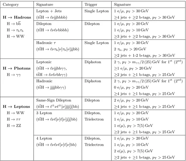
The experimental searches for ttH production presented here can be divided into three broad categories based on the Higgs boson signatures: H → hadrons, H → photons, and H → leptons. There are two main Higgs boson decay modes that contribute to the H → hadrons searches: H → bb and H → τ τ , where both τ leptons decay hadronically. Note that events with τ pairs include both direct H → τ τ decays and those where the τ leptons are produced by the decays of W or Z bosons from H → WW and H → ZZ decays. Events used in the H → hadrons searches have one or more isolated charged lepton from the W boson decays from the top quarks, which means these searches focus on the lepton + jets and dilepton tt final states, using single-lepton or dilepton triggers, respectively. Multivariate analysis (MVA) techniques are employed to tag the jets coming from b-quark or τ -lepton decays and to separate ttH events from the large tt+jets backgrounds.

In contrast, the H → photons search focuses exclusively on the H → γγ decay mode. In this case, the photons provide the trigger, and all three tt decay topologies are included in the analysis. The CMS detector’s excellent γγ invariant mass resolution [31] is used to separate the ttH signal from the background, and the background model is entirely based on data.

Finally, in the H → leptons search, the leptons arise as secondary decay products from H → WW, H → ZZ, and H → τ τ decays, as well as from the W bosons produced in the top quark decays. To optimize the signal-to-background ratio, events are required to have either a pair of same-sign charged leptons, or three or more charged leptons. The events are required to pass the dilepton or trilepton triggers. Multivariate analysis techniques are used to separate leptons arising from W-boson, Z-boson and τ -lepton decays, referred to as signal leptons, from background leptons, which come from b-quark or c-quark decays, or misiden-tified jets. MVA techniques are also used to distinguish ttH signal events from background events that are modeled using a mixture of control samples in data and Monte Carlo (MC) simulation. Table 1summarizes the main features of each search channel described above. To characterize the strength of the ttH signal relative to the SM cross section (µ = σ/σSM) a fit is performed simultaneously in all channels. The fit uses specific discriminating

distributions in each channel, either a kinematic variable like the diphoton invariant mass in the H → photons channel or an MVA discriminant as in the H → hadrons and H →

(5)

JHEP09(2014)087

Category Signature Trigger Signature

Lepton + Jets Single Lepton 1 e/µ, pT> 30 GeV

H → Hadrons (ttH → `νjjbbbb) ≥4 jets + ≥2 b-tags, pT> 30 GeV

H → bb Dilepton Dilepton 1 e/µ, pT> 20 GeV

H → τhτh (ttH → `ν`νbbbb) 1 e/µ, pT> 10 GeV

H → WW ≥3 jets + ≥2 b-tags, pT> 30 GeV

Hadronic τ Single Lepton 1 e/µ, pT> 30 GeV

(ttH → `ντh[ν]τh[ν]jjbb) 2 τh, pT> 20 GeV

≥2 jets + 1-2 b-tags, pT> 30 GeV

Leptonic Diphoton 2 γ, pT> mγγ/2 (25) GeV for 1st(2nd)

H → Photons (ttH → `νjjbbγγ, ≥1 e/µ, pT> 20 GeV

H → γγ ttH → `ν`νbbγγ) ≥2 jets + ≥1 b-tags, pT> 25 GeV

Hadronic Diphoton 2 γ, pT> mγγ/2 (25) GeV for 1st(2nd)

(ttH → jjjjbbγγ) 0 e/µ, pT> 20 GeV

≥4 jets + ≥1 b-tags, pT> 25 GeV

Same-Sign Dilepton Dilepton 2 e/µ, pT> 20 GeV

H → Leptons (ttH → `±ν`±[ν]jjj[j]bb) ≥4 jets + ≥1 b-tags, pT> 25 GeV

H → WW 3 Lepton Dilepton, 1 e/µ, pT> 20 GeV

H → τ τ (ttH → `ν`[ν]`[ν]j[j]bb) Trielectron 1 e/µ, pT> 10 GeV

H → ZZ 1 e(µ), pT> 7(5) GeV

4 Lepton Dilepton, 1 e/µ, pT> 20 GeV

(ttH → `ν`ν`[ν]`[ν]bb) Trielectron 1 e/µ, pT> 10 GeV

2 e(µ), pT> 7(5) GeV

Table 1. Summary of the search channels used in the ttH analysis. In the description of the signatures, an ` refers to any electron or muon in the final state (including those coming from leptonic τ decays). A hadronic τ decay is indicated by τh. Finally, j represents a jet coming from

any quark or gluon, or an unidentified hadronic τ decay, while b represents a b-quark jet. Any element in the signature enclosed in square brackets indicates that the element may not be present, depending on the specific decay mode of the top quark or Higgs boson. The minimum transverse momentum pT of various objects is given to convey some sense of the acceptance of each search

channel; however, additional requirements are also applied. Jets labeled as b-tagged jets have been selected using the algorithm described in section4. More details on the triggers used to collect data for each search channel are given in section3. Selection of final-state objects (leptons, photons, jets, etc.) is described in general in section4, with further channel-specific details included in sections5–

7. In this table and the rest of the paper, the number of b-tagged jets is always included in the jet count. For example, the notation 4 jets + 2 b-tags means four jets of which two jets are b-tagged.

(6)

JHEP09(2014)087

leptons cases. The uncertainties involved in the background modeling are introduced in the fit as nuisance parameters, so that the best-fit parameters provide an improved description of the background.

This paper is structured as follows. Sections 2 and 3 describe the CMS detector, and the data and simulation samples, respectively. Section 4 discusses the common ob-ject reconstruction and identification details shared among the different search channels. Sections 5, 6, and 7 outline the selection, background modeling, and signal extraction techniques for the H → hadrons, H → photons, and H → leptons analyses, respectively. Section8details the impact of systematic uncertainties on the searches. Finally, the combi-nation procedure and results are presented in section9, followed by a summary in section10.

2 The CMS detector

The central feature of the CMS apparatus is a superconducting solenoid of 6 m internal diameter, providing an axial magnetic field of 3.8 T parallel to the beam direction. Within the superconducting solenoid volume, there are a silicon pixel and strip tracker, a lead tungstate crystal electromagnetic calorimeter (ECAL), and a brass/scintillator hadron cal-orimeter (HCAL). The tracking detectors provide coverage for charged particles within |η| < 2.5. The ECAL and HCAL calorimeters provide coverage up to |η| < 3.0. The ECAL is divided into two distinct regions: the barrel region, which covers |η| < 1.48, and the end-cap region, which covers 1.48 < |η| < 3.0. A quartz-fiber forward calorimeter extends the coverage further up to |η| < 5.0. Muons are measured in gas-ionization detectors embedded in the steel flux-return yoke outside the solenoid. The first level (L1) of the CMS trigger system, composed of custom hardware processors, uses information from the calorimeters and muon detectors to select the most interesting events in a fixed time interval of less than 4 µs. The high-level trigger (HLT) processor farm further decreases the event rate from around 100 kHz to less than 1 kHz, before data storage. A more detailed description of the CMS detector, together with a definition of the coordinate system used and the relevant kinematic variables, can be found in ref. [18].

3 Data and simulation samples

This search is performed with samples of proton-proton collisions at√s = 7 TeV, collected with the CMS detector in 2011 (referred to as the 7 TeV dataset), and at √s = 8 TeV, collected in 2012 (referred to as the 8 TeV dataset). All of the search channels make use of the full CMS 8 TeV dataset, corresponding to an integrated luminosity that ranges from 19.3 fb−1 to 19.7 fb−1, with a 2.6% uncertainty [32]. The luminosity used varies slightly because the different search channels have slightly different data quality requirements, de-pending on the reconstructed objects and triggers used. In addition, the H → photons anal-ysis makes use of data collected at√s = 7 TeV, corresponding to an integrated luminosity of 5.1 fb−1. Finally, the ttH search in the H → bb final state based on the 7 TeV dataset with an integrated luminosity of 5.0 fb−1, described in ref. [33], is combined with the 8 TeV analysis to obtain the final ttH result. The uncertainty on the 7 TeV luminosity is 2.2% [34].

(7)

JHEP09(2014)087

In the H → hadrons and H → leptons analyses, events are selected by triggering on the presence of one or more leptons. For the H → photons analysis, diphoton triggers are used. Single-lepton triggers are used for channels with one lepton in the final state. The single-electron trigger requires the presence of an isolated, good-quality electron with trans-verse momentum pT > 27 GeV. The single-muon trigger requires a muon candidate isolated

from other activity in the event with pT> 24 GeV. Dilepton triggers are used for channels

with two or more leptons in the final state. The dilepton triggers require any combination of electrons and muons, one lepton with pT > 17 GeV and another with pT > 8 GeV. In

the H → leptons analysis, a trielectron trigger is used, with minimum pT thresholds of

15 GeV, 8 GeV, and 5 GeV. The H → photons analysis uses diphoton triggers with two different photon identification schemes. One requires calorimetric identification based on the electromagnetic shower shape and isolation of the photon candidate. The other re-quires only that the photon has a high value of the R9 shower shape variable, where R9 is

calculated as the ratio of the energy contained in a 3×3 array of ECAL crystals centered on the most energetic deposit in the supercluster to the energy of the whole supercluster. The superclustering algorithm for photon reconstruction is explained in more detail in sec-tion4. The ET thresholds at trigger level are 26 (18) GeV and 36 (22) GeV on the leading

(trailing) photon depending on the running period. To maintain high trigger efficiency, all four combinations of thresholds and selection criteria are used.

Expected signal events and, depending on the analysis channel, some background pro-cesses are modeled with MC simulation. The ttH signal is modeled using the pythia gen-erator [35] (version 6.4.24 for the 7 TeV dataset and version 6.4.26 for the 8 TeV dataset). Separate samples were produced at nine different values of mH: 110, 115, 120, 122.5, 125,

127.5, 130, 135, and 140 GeV, and are used to interpolate for intermediate mass values. The background processes ttW, ttZ, tt+jets, Drell-Yan+jets, W+jets, ZZ+jets, WW+jets, and WZ+jets are all generated with the MadGraph 5.1.3 [36] tree-level matrix element generator, combined with pythia for the parton shower and hadronization. For the H → leptons analysis, the rare WWZ, WWW, tt + γ+jets, and ttWW processes are generated similarly. Single top quark production (t+q, t+b, and t+W) is modeled with the next-to-leading-order (NLO) generator powheg 1.0 [37–42] combined with pythia. Samples that include top quarks in the final state are generated with a top quark mass of 172.5 GeV. For the H → photons analysis, the gluon fusion (gg → H) and vector boson fusion (qq → qqH) production modes are generated with powheg at NLO, and combined with pythia for the parton shower and hadronization. Higgs boson production in association with weak bosons (qq → WH/ZH) is simulated with pythia. Samples generated with a leading order generator use the CTEQ6L1 parton distribution function (PDF) [43] set, while samples generated with NLO generators use the CTEQ6.6M PDF set [44].

The CMS detector response is simulated using the Geant4 software package [45]. All events from data and simulated samples are required to pass the same trigger conditions and are reconstructed with identical algorithms to those used for collision data. Effects from additional pp interactions in the same bunch crossing (pileup) are modeled by adding simulated minimum bias events (generated with pythia) to the generated hard interac-tions. The pileup interaction multiplicity distribution in simulation reflects the luminosity

(8)

JHEP09(2014)087

profile observed in pp collision data. Additional correction factors are applied to individual object efficiencies and energy scales to bring the MC simulation into better agreement with data, as described in section4.

4 Object reconstruction and identification

A global event description is obtained with the CMS particle-flow (PF) algorithm [46,47], which optimally combines the information from all CMS sub-detectors to reconstruct and identify each individual particle in the pp collision event. The particles are classified into mutually exclusive categories: charged hadrons, neutral hadrons, photons, muons, and elec-trons. The primary collision vertex is identified as the reconstructed vertex with the highest value ofP p2

T, where the summation includes all particles used to reconstruct the vertex.

Although the separate ttH search channels share the same overall object reconstruction and identification approach, there are differences in some of the selection requirements. Generally speaking, the requirements in the H → hadrons channel are more stringent than in the H → photons or leptons because of the larger backgrounds in the first channel and the smaller amount of signal in the other ones.

Photon candidates are reconstructed from the energy deposits in the ECAL, grouping the individual clusters into a supercluster. The superclustering algorithms achieve an almost complete reconstruction of the energy of photons (and electrons) that convert into electron-positron pairs (emit bremsstrahlung) in the material in front of the ECAL. In the barrel region, superclusters are formed from five-crystal-wide strips in η, centered on the locally most energetic crystal (seed), and have a variable extension in φ. In the endcaps, where the crystals are arranged according to an x-y rather than an η-φ geometry, matrices of 5×5 crystals (which may partially overlap) around the most energetic crystals are merged if they lie within a narrow φ road. The photon candidates are collected within the ECAL fiducial region |η| < 2.5, excluding the barrel-endcap transition region 1.44 < |η| < 1.57 where photon reconstruction is sub-optimal. Isolation requirements are applied to photon candidates by looking at neighboring particle candidates reconstructed with the PF event reconstruction technique [46]. Additional details on photon reconstruction and identification can be found in ref. [30].

Electrons with pT > 7 GeV are reconstructed within the geometrical acceptance of the

tracker, |η| < 2.5. The reconstruction combines information from clusters of energy deposits in the ECAL and the electron trajectory reconstructed in the inner tracker [48–51]. The track-cluster matching is initiated either “outside-in” from ECAL clusters, or “inside-out” from track candidates. Trajectories in the tracker volume are reconstructed using a dedi-cated modeling of the electron energy loss and fitted with a Gaussian sum filter [48]. The electron momentum is determined from the combination of ECAL and tracker measure-ments. Electron identification relies on a multivariate technique that combines observables sensitive to the amount of bremsstrahlung along the electron trajectory, the spatial and momentum matching between the electron trajectory and associated clusters, and shower shape observables. In order to increase the lepton efficiency, the H → leptons analysis uses a looser cut on the multivariate discriminant than do the other analysis channels.

(9)

Al-JHEP09(2014)087

though the minimum pT requirement on electrons is pT > 7 GeV, the different ttH search

channels, particularly the H → hadrons channel, use a higher threshold on some of the selected electrons depending on the trigger requirements and to help control backgrounds (see sections 5–7 for more details).

Muons are reconstructed within |η| < 2.4 and for pT> 5 GeV [52]. The reconstruction

combines information from both the silicon tracker and the muon spectrometer. The matching between the inner and outer tracks is initiated either “outside-in”, starting from a track in the muon system, or “inside-out”, starting from a track in the silicon tracker. The PF muons are selected among the reconstructed muon track candidates by applying minimal requirements on the track components in the muon and tracker systems and taking into account matching with energy deposits in the calorimeters [53]. Depending on the level of backgrounds in a given analysis channel, different requirements can be placed on the distance of closest approach for the muon to the collision vertex — referred to as the impact parameter (IP)—in both the z−direction (dz) and the x − y plane (dxy) to reject

background muons. As in the electron case, the pT threshold for some or all of the muons

is set higher than the 5 GeV default, depending on the trigger requirements used by a particular search channel and to control backgrounds.

An important quantity for distinguishing signal and background leptons is isolation. Although conceptually similar, isolation is defined slightly differently for muons and elec-trons depending on the analysis channel. Muon isolation is assessed by calculating the sum of the transverse energy of the other particles in a cone of ∆R = p(∆η)2_{+ (∆φ)}2 _{= 0.4}

around the muon direction, excluding the muon itself, where ∆η and ∆φ are the angular differences between the muon and the other particles in the η and φ directions. To correct for the effects of pileup, charged contributions not originating from the primary collision vertex are explicitly removed from the isolation sum, and the neutral contribution is cor-rected assuming a ratio of 0.5 for the contribution of neutral to charged objects to the pileup activity. The ratio of the corrected isolation sum to the muon pT is the relative

isolation of the muon. For the H → leptons search, electron isolation is calculated identi-cally to muon isolation. For the H → hadrons and H → photons searches, there are two differences. The first is that the electron isolation sum only takes into account charged and neutral particles in a cone of ∆R = 0.3. Second, the correction for pileup effects to the neutral contribution in the isolation sum is made using the average pT density calculated

from neutral particles multiplied by the effective area of the isolation cone. The relative isolation is the ratio of this corrected isolation sum to the electron pT.

Jets are reconstructed by clustering the charged and neutral PF particles using the anti-kT algorithm with a distance parameter of 0.5 [54,55]. For the H → hadrons search,

particles identified as isolated muons and electrons are expected to come from W-boson decays and are excluded from the clustering. Non-isolated muons and electrons are expected to come from b-quark decays and are included in the clustering. The H → leptons and H → photons searches do not exclude the isolated leptons from the jet clustering, but require selected jets to be separated by ∆R > 0.5 from the selected leptons. The choice not to exclude leptons from the clustered jets in the H → leptons search is an integral part of the non-prompt lepton rejection strategy. When a lepton is clustered into a jet, that

(10)

JHEP09(2014)087

information is used to help determine whether the lepton originated from a semileptonic decay of a heavy (bottom or charm) quark (see section 7for more details).

Jets are required to have at least two PF constituents and more than 1% of their energy in both the electromagnetic and hadronic components to reject jets arising from instru-mental effects. For the H → leptons and H → photons searches, additional requirements are applied to remove jets coming from pileup vertices [56]. For the H → hadrons and H → leptons analyses, charged PF particles not associated with the primary event vertex are ignored when clustering the jets to reduce the contribution from pileup. The momentum of the clustered jet is corrected for a variety of effects [57]. The component coming from pileup activity — in the case of H → hadrons or leptons, just the neutral part — is removed by applying a residual energy correction following the area-based procedure described in refs. [58,59]. Further corrections based on simulation, γ/Z+jets data, and dijet data are then applied, as well as a correction to account for residual differences between data and simulation [57]. Selected jets are required to have |η| < 2.4, and pT> 25 GeV (H → leptons

and H → photons) or pT > 30 GeV (H → hadrons). The higher pT requirement in the

latter case arises from the larger amount of background in that sample.

Jets are identified as originating from a b-quark using the combined secondary vertex (CSV) algorithm [60, 61] that utilizes information about the impact parameter of tracks and reconstructed secondary vertices within the jets in a multivariate algorithm. The CSV algorithm provides a continuous output ranging from 0 to 1; high values of the CSV discriminant indicate that the jet likely originates from a b quark, while low values indicate the jet is more consistent with light-flavor quarks or gluons. The efficiency to tag b-quark jets and the rate of misidentification of non-b-quark jets depend on the working point chosen. For the medium working point of the CSV algorithm, the b-tagging efficiency is around 70% (20%) for jets originating from a b (c) quark and the probability of mistagging for jets originating from light quarks or gluons is approximately 2%. For the loose working point, the efficiency to tag jets from b (c) quarks is approximately 85% (40%) and the probability to tag jets from light quarks or gluons is about 10%. These efficiencies and mistag probabilities vary with the pTand η of the jets, and the values quoted are indicative

of the predominant jets in this analysis.

The hadronic decay of a τ lepton (τh) produces a narrow jet of charged and

neu-tral hadrons — almost all pions. Each neuneu-tral pion subsequently decays into a pair of photons. The identification of τh jets begins with the formation of PF jets by clustering

charged hadron and photon objects via the anti-kTalgorithm. Then, the hadron-plus-strips

(HPS) [62,63] algorithm tests each of the most common τh decay mode hypotheses using

the electromagnetic objects found within rectangular bands along the azimuthal direc-tion. In the general algorithm, combinations of charged hadrons and photons (one charged hadron, one charged hadron + photons, and three charged hadrons) must lead to invariant masses consistent with the appropriate intermediate resonances [63]. For this analysis, only the decays involving exactly one charged hadron are used.

The missing transverse energy vector is calculated as the negative vector pT sum of all

PF candidates identified in the event. The magnitude of this vector is denoted as Emiss_T . Since pileup interactions degrade the performance of the Emiss_T variable, the H → leptons

(11)

JHEP09(2014)087

search also uses the H_Tmiss variable. This variable is computed in the same way as the E_Tmiss, but uses only the selected jets and leptons. The H_Tmiss variable has worse resolution than E_Tmiss but it is more robust as it does not rely on soft objects in the event. A linear discriminator is computed based on the two variables,

LD= 0.60ETmiss+ 0.40HTmiss, (4.1)

exploiting the fact that E_Tmissand H_Tmissare less correlated in events with missing transverse energy from instrumental mismeasurement than in events with genuine missing transverse energy. The linear discriminant is constructed to optimize separation between ttH and Z+jets in simulation.

To match the performance of reconstructed objects between data and simulation, the latter is corrected with the following data-MC scale factors: leptons are corrected for the difference in trigger efficiency, as well as in lepton identification and isolation efficiency. For the H → leptons channel, corrections accounting for residual differences between data and simulation are applied to the muon momentum, as well as to the ECAL energy before combining with the tracking momentum for electrons. All lepton corrections are derived using tag-and-probe techniques [64] based on samples with Z boson and J/ψ decays into two leptons. Jet energy corrections as described above are applied as a function of the jet pT and η [57]. Standard efficiency scale factors for the medium and loose b-tagging

working points [60,61] are applied for light- and heavy-flavor jets in the H → leptons and H → photons searches, while the H → hadrons search uses a more sophisticated correction to the CSV shape (see section5 for more details).

5 H → hadrons

5.1 Event selection

Events in the H → hadrons analysis are split into three different channels based on the decay modes of the top-quark pair and the Higgs boson: the lepton+jets channel (tt → `νqq0bb, H → bb), the dilepton channel (tt → `+ν`−νbb, H → bb), and the τh channel

(tt → `νqq0bb, H → τhτh), where a lepton is an electron or a muon. For the lepton+jets

channel, events containing an energetic, isolated lepton, and at least four energetic jets, two or more of these jets must be b-tagged, are selected. For the dilepton channel, a pair of oppositely charged leptons and three or more jets, with at least two of the jets being b-tagged, are required. For the τhchannel, beyond the two identified hadronically decaying

τ leptons, at least two jets, one or two of which must be b-tagged, are required. The event selections are designed to be mutually exclusive. For all figures (figures 2–7) and tables (tables 2–4) of the H → hadrons analysis, the b-tagged jets are included in the jet count.

In addition to the baseline selection detailed in section4, two additional sets of selection criteria are applied to leptons in the H → hadrons analysis: tight and loose, described below. All events are required to contain at least one tight electron or muon. Loose requirements are only applied to the second lepton in the dilepton channel.

Tight and loose muons differ both in the identification and kinematic requirements. For events in the lepton+jets and τh channels, tight muons are required to have pT > 30 GeV

(12)

JHEP09(2014)087

and |η| < 2.1 to ensure that the trigger is fully efficient with respect to the offline selection. Tight muons in the dilepton channel have a lower pT threshold at 20 GeV. Loose muons

must have pT > 10 GeV and |η| < 2.4. For tight (loose) muons, the relative isolation is

required to be less than 0.12 (0.2). Tight muons must also satisfy additional quality criteria based on the number of hits associated with the muon candidate in the pixel, strip, and muon detectors. To ensure the muon is from a W decay, it is required to be consistent with originating from the primary vertex with an impact parameter in the x − y plane dxy < 0.2 cm and distance from the primary vertex in the z-direction dz < 0.5 cm. For

loose muons, no additional requirements beyond the baseline selection are applied.

Tight electrons in the lepton+jets and τh channels are required to have pT > 30 GeV,

while the dilepton channel requires pT > 20 GeV. Loose electrons are required to have

pT > 10 GeV. All electrons must have |η| < 2.5, and those that fall into the transition

region between the barrel and endcap of the ECAL (1.44 < |η| < 1.57) are rejected. Tight electrons must have a relative isolation less than 0.1, while loose electrons must have a rela-tive isolation less than 0.2. In a manner similar to tight muons, tight electrons are required to have dxy < 0.02 cm and dz < 1 cm, while loose electrons must have dxy < 0.04 cm.

For τ leptons decaying hadronically, only candidates with well-reconstructed decay modes [63] that contain exactly one charged pion are accepted. Candidates must have pT > 20 GeV and |η| < 2.1, and the pT of the charged pion must be greater than 5 GeV.

Candidates are additionally required to fulfill criteria that reject electrons and muons mimicking hadronic τ -lepton decays. These include requirements on the consistency of information from the tracker, calorimeters, and muon detectors, including the absence of large energy deposits in the calorimeters for muons and bremsstrahlung pattern recognition for electrons. A multivariate discriminant, which takes into account the effects of pileup, is used to select loosely isolated τh candidates [65]. Finally, the τh candidates must be

separated from the single tight muon or electron in the event by a distance ∆R > 0.25. Events are required to contain at least one pair of oppositely charged τhcandidates. In the

case that multiple valid pairs exist, the pair with the most isolated τh signatures, based on

the aforementioned MVA discriminant, is chosen.

While the basic jet pT threshold is 30 GeV, in the lepton+jets channel, the leading

three jets must have pT > 40 GeV. Jets originating from b quarks are identified using the

CSV medium working point.

5.2 Background modeling

All the backgrounds in the H → hadrons analysis are normalized using NLO or better inclusive cross section calculations [66–71]. To determine the contribution of individual physics processes to exclusive final states as well as to model the kinematics, the MC simulations described in section 3 are used. The main background, tt+ jets, is generated using MadGraph inclusively, with tree-level diagrams for up to tt+3 extra partons. These extra partons include both b and c quarks. However, as there are significantly different uncertainties in the production of additional light-flavor (lf) jets compared to heavy-flavor (hf), the tt+jets sample is separated into subsamples based on the quark flavor associated with the reconstructed jets in the event. Events where at least two reconstructed jets are

(13)

JHEP09(2014)087

matched at the generator level to extra b quarks (that is b quarks not originating from a top-quark decay) are labeled as tt + bb events. If only a single jet is matched to a b quark, the event is classed as tt+b. These cases typically arise because the second extra b quark in the event is either too far forward or too soft to be reconstructed as a jet, or the two extra b quarks have merged into a single jet. Finally, if at least one reconstructed jet is matched to a c quark at the generator level, the event is labeled as tt + cc. Different systematic uncertainties affecting both rates and shapes are applied to each of the separate subsets of the tt+jets sample, as described in section 8.

Besides the common corrections to MC samples described in section 4, additional cor-rection factors are applied for samples modeling the backgrounds for this analysis channel. A correction factor to tt+jets MC samples is applied so that the top-quark pT spectrum

from MadGraph agrees with the distribution observed in data and predicted by higher-order calculations. These scale factors, which range from roughly 0.75 to 1.2, were derived from a fully corrected measurement of the tt differential cross section as function of the top-quark pT using the

√

s = 8 TeV dataset obtained using the same techniques as described in ref. [72].

Furthermore, a dedicated correction to the CSV b-tagging rates is applied to all the MC samples. The CSV discriminant is used to identify b-quark jets, and the CSV dis-criminant shape is used in the signal extraction technique to distinguish between events with additional genuine b-quark jets and those with mistags. Therefore, a correction for the efficiency difference between data and simulation over the whole range of discriminator values is applied. The scale factors — which are between 0.7 and 1.3 for the bulk of the jets — are derived separately for light-flavor (including gluons) and b-quark jets using two independent samples of 8 TeV data in the dilepton channel. Both control samples are also orthogonal to the events used in the signal extraction. The light-flavor scale factor deriva-tion uses a control sample enriched in events with a Z boson, selected by requiring a pair of opposite-charge, same-flavor leptons and exactly two jets. The b-quark scale factor is de-rived in a sample dominated by dileptonic tt, a signature that includes exactly two b-quark jets, by selecting events with two leptons that are not consistent with a Z boson decay and exactly two jets. Using these control samples, a tag-and-probe approach is employed where one jet (“tag”) passes the appropriate b-tagging requirement for a light-flavor or b-quark jet. The CSV discriminant of the other jet (“probe”) is compared between the data and simulation, and the ratio gives a scale factor for each jet as a function of CSV discriminant value, pT and η. Each light-flavor or b-quark jet is then assigned an appropriate individual

scale factor. The CSV output shape for c-quark jets is dissimilar to that of both light-flavor and b-quark jets; hence, in the absence of a control sample of c-quark jets in data, a scale factor of 1 is applied, with twice the relative uncertainty ascertained from b-quark jets (see section 8). These CSV scale factors are applied to simulation on an event-by-event basis where the overall scale factor is the product of the individual scale factors for each jet in the event. This procedure was checked using control samples.

Tables2,3, and 4show the predicted event yields compared to data after the selection in the lepton+jets, dilepton, and τh channels, respectively. The tables are sub-divided into

(14)

JHEP09(2014)087

≥6 jets + 4 jets + 5 jets + ≥6 jets + 4 jets + 5 jets + ≥6 jets +

2 b-tags 3 b-tags 3 b-tags 3 b-tags 4 b-tags ≥4 b-tags ≥4 b-tags ttH(125.6 GeV) 28.5 ± 2.5 12.4 ± 1.0 18.1 ± 1.5 18.9 ± 1.5 1.5 ± 0.2 4.4 ± 0.4 6.7 ± 0.6 tt+lf 7140 ± 310 4280 ± 150 2450 ± 130 1076 ± 74 48.4 ± 10.0 54 ± 12 44 ± 11 tt+b 570 ± 170 364 ± 94 367 ± 98 289 ± 87 20.0 ± 5.5 28.6 ± 8.0 33 ± 10 tt + bb 264 ± 59 123 ± 29 193 ± 42 232 ± 49 15.8 ± 3.6 45.2 ± 9.7 86 ± 18 tt + cc 2420 ± 300 690 ± 130 800 ± 130 720 ± 110 29.7 ± 5.6 55 ± 11 81 ± 13 tt+W/Z 85 ± 11 15.0 ± 2.0 20.9 ± 2.8 24.7 ± 3.3 1.0 ± 0.2 2.1 ± 0.4 4.7 ± 0.8 Single t 236 ± 18 213 ± 17 101.7 ± 10.0 47.7 ± 6.7 2.8 ± 1.4 7.5 ± 3.8 6.7 ± 2.6 W/Z+jets 75 ± 27 46 ± 30 13 ± 12 7.7 ± 8.8 1.1 ± 1.2 0.9 ± 1.0 0.3 ± 0.8 Diboson 4.5 ± 1.0 5.4 ± 0.9 2.0 ± 0.5 1.0 ± 0.4 0.2 ± 0.2 0.1 ± 0.1 0.2 ± 0.1 Total bkg 10790 ± 200 5730 ± 110 3935 ± 74 2394 ± 65 119.0 ± 8.2 193.4 ± 10.0 256 ± 16 Data 10724 5667 3983 2426 122 219 260

Table 2. Expected event yields for signal (mH= 125.6 GeV) and backgrounds in the lepton+jets

channel. Signal and background normalizations used for this table are described in the text.

prediction (µ fixed to 1). In these tables, background yields and uncertainties use the best-fit value of all nuisance parameters, with µ fixed at 1. For more details about the statistical treatment and the definition of µ, see section 9. The expected and observed yields agree well in all final states across the different jet and b-tag categories.

Figures2,3, and4 show the data-to-simulation comparisons of variables that give the best signal-background separation in each of the lepton+jets, dilepton, and τh channels,

respectively. In these plots, the background is normalized to the SM expectation; the uncertainty band (shown as a hatched band in the stack plot and a green band in the ratio plot) includes statistical and systematic uncertainties that affect both the rate and shape of the background distributions. For the ratio plots shown below each distribution, only the background expectation (and not the signal) is included in the denominator of the ratio. The contribution labeled “EWK” is the sum of the diboson and W/Z+jets backgrounds. The ttH signal (mH= 125.6 GeV) is not included in the stacked histogram, but is shown

as a separate open histogram normalized to 30 times the SM expectation (µ = 30). To calculate the variable second m(jj,H), the invariant masses of all jet pairs with at least one b-tagged jet are calculated and the jet pair whose mass is the second closest to the Higgs boson mass is chosen. Within the uncertainties, the simulation reproduces well the shape and the normalization of the distributions.

5.3 Signal extraction

Boosted decision trees (BDTs) [73] are used to further improve signal sensitivity. In the lepton+jets and dilepton channels, BDTs are trained separately for each category, using the ttH sample with mH= 125 GeV. The three dilepton categories use a single BDT. Of

the seven lepton+jets categories, four categories use a single BDT, while three categories each use two BDTs in a tiered configuration. The tiered configuration includes one BDT that is trained specifically to discriminate between ttH and ttbb events, the output of which

(15)

JHEP09(2014)087

(lepton,jets,MET) (GeV) T Sum p 0 200 400 600 800 1000 1200 1400 1600 Events 500 1000 1500 2000 2500 3000 -1 = 8 TeV, L = 19.3 fb s b CMS ttH b

Lepton + 4 jets + 3 b-tags

(lepton,jets,MET) (GeV) T Sum p 0 200 400 600 800 1000 1200 1400 1600 Data/MC 0 1 2

highest CSV output of b-tagged jets

rd 3 0.7 0.75 0.8 0.85 0.9 0.95 1 Events 10 20 30 40 50 -1 = 8 TeV, L = 19.3 fb s b CMS ttH b

rd 3 0.7 0.75 0.8 0.85 0.9 0.95 1 Data/MC 0 1 2 H(125.6) x 30 t t + lf t t c + c t t + b t t b + b t t Single t + W,Z t t EWK Bkg. Unc. Data (lepton,jets,MET) (GeV) T Sum p 0 200 400 600 800 1000 1200 1400 Events 200 400 600 800 1000 1200 1400 1600 1800 -1 = 8 TeV, L = 19.3 fb s b CMS ttH b

(lepton,jets,MET) (GeV) T Sum p 0 200 400 600 800 1000 1200 1400 Data/MC 0 1

2 0.75 0.8 0.85 _{Average CSV output (b-tags)}0.9 0.95 1

Events 10 20 30 40 50 60 -1 = 8 TeV, L = 19.3 fb s b CMS ttH b 4 b-tags ≥ Lepton + 5 jets +

Average CSV output (b-tags)

0.75 0.8 0.85 0.9 0.95 1

Data/MC

0 1 2

rd 3 0 0.2 0.4 0.6 0.8 1 Events 200 400 600 800 1000 1200 1400 1600 1800 2000 -1 = 8 TeV, L = 19.3 fb s b CMS ttH b 6 jets + 2 b-tags ≥ Lepton +

rd 3 0 0.2 0.4 0.6 0.8 1 Data/MC 0 1

2 0.75 0.8 0.85_{Average CSV output (b-tags)}0.9 0.95 1

Events 100 200 300 400 500 -1 = 8 TeV, L = 19.3 fb s b CMS ttH b 6 jets + 3 b-tags ≥ Lepton +

0.75 0.8 0.85 0.9 0.95 1

Data/MC

0 1

2 0.75 0.8 0.85 _{Average CSV output (b-tags)}0.9 0.95 1

Events 10 20 30 40 50 60 70 -1 = 8 TeV, L = 19.3 fb s b CMS ttH b 4 b-tags ≥ 6 jets + ≥ Lepton +

0.75 0.8 0.85 0.9 0.95 1

Data/MC

0 1 2

Figure 2. Input variables that give the best signal-background separation for each of the lep-ton+jets categories used in the analysis at √s = 8 TeV. The top, middle, and bottom rows show the events with 4, 5, and ≥6 jets, respectively, while the left, middle, and right columns are events with 2, 3, and ≥4 b-tags, respectively. More details regarding these plots are found in the text.

(16)

JHEP09(2014)087

+ lf t

t tt + cc tt + b tt + bb

Single t tt + W,Z EWK Bkg. Unc.

Data ttH(125.6) x 30 200 300 400 500 600 700 Events 500 1000 1500 2000 2500

3000 Dilepton + 3 jets + 2 b-tags

-1 = 8 TeV, L = 19.3 fb s b CMS ttH b

(lepton, jets) (GeV)

T Sum p 200 300 400 500 600 700 Data/MC 0 1 2 4 4.5 5 5.5 6 6.5 7 7.5 8 Events 500 1000 1500 2000 2500 3000 3500

4000 Dilepton + ≥4 jets + 2 b-tags

-1 = 8 TeV, L = 19.3 fb s b CMS ttH b Number of jets 4 4.5 5 5.5 6 6.5 7 7.5 8 Data/MC 0 1 2 60 80 100 120 140 160 180 200 220 240 Events 20 40 60 80 100 120 140 160 180 200 3 b-tags ≥ 3 jets + ≥ Dilepton + -1 = 8 TeV, L = 19.3 fb s b CMS ttH b Second m(jj,H) (GeV) 60 80 100 120 140 160 180 200 220 240 Data/MC 0 1 2

Figure 3. Input variables that give the best signal-background separation for each of the dilepton categories used in the analysis at √s = 8 TeV. The left, middle, and right panels show the events with 3 jets and 2 b-tags, ≥4 jets and 2 b-tags, and ≥3 b-tags, respectively. More details regarding these plots are found in the text.

H(125.6) x 30 t t t t Single t + W,Z t t EWK Bkg. Unc. Data (GeV) T p h τ More energetic 20 30 40 50 60 70 80 90 100 Events 20 40 60 80 100 2 jets + 1-2 b-tags ≥ + h τ h τ Lep + CMS ttHτhτh s = 8 TeV, L = 19.3 fb-1 (GeV) T p h τ More energetic 20 30 40 50 60 70 80 90 100 Data/MC 0 0.5 1 1.5 2 Mvis (GeV) 0 20 40 60 80 100 120 140 160 180 200 Events 10 20 30 40 50 60 70 80

90 Lep + τhτh + ≥ 2 jets + 1-2 b-tags

CMS ttHτhτh s = 8 TeV, L = 19.3 fb-1 (GeV) vis M 0 20 40 60 80 100 120 140 160 180 200 Data/MC 0 0.5 1 1.5 2

Figure 4. Examples of input variables that give the best signal-background separation in the analysis of the τh channels at

√

s = 8 TeV. The left plot shows the pT of the more energetic τh,

while the right plot displays Mvis, the mass of the visible τhdecay products. Events of all categories

(17)

JHEP09(2014)087

3 jets + 2 b-tags ≥4 jets + 2 b-tags ≥3 b-tags

ttH(125.6 GeV) 7.4 ± 0.6 14.5 ± 1.2 10.0 ± 0.8 tt+lf 7650 ± 170 3200 ± 120 227 ± 35 tt+b 210 ± 55 198 ± 57 160 ± 43 tt + bb 50 ± 13 76 ± 17 101 ± 21 tt + cc 690 ± 110 761 ± 97 258 ± 46 tt+W/Z 29.5 ± 3.8 50.5 ± 6.4 10.9 ± 1.5 Single t 218 ± 16 95.2 ± 8.8 14.6 ± 3.6 W/Z+jets 217 ± 52 98 ± 28 21 ± 15 Diboson 9.5 ± 0.9 2.9 ± 0.4 0.6 ± 0.1 Total bkg 9060 ± 130 4475 ± 82 793 ± 28 Data 9060 4616 774

Table 3. Expected event yields for signal (mH = 125.6 GeV) and backgrounds in the dilepton

channel. Signal and background normalizations used for this table are described in the text.

2 jets + 3 jets + ≥4 jets + 2 jets + 3 jets + ≥4 jets +

1 b-tag 1 b-tag 1 b-tag 2 b-tags 2 b-tags 2 b-tags

ttH(125.6 GeV) 0.4 ± 0.1 0.6 ± 0.1 0.5 ± 0.1 0.1 ± 0.0 0.2 ± 0.0 0.3 ± 0.0 tt+lf 266 ± 12 144.7 ± 7.1 72.1 ± 4.1 55.0 ± 3.4 45.2 ± 2.8 28.8 ± 2.1 tt+W/Z 1.1 ± 0.2 1.3 ± 0.2 1.3 ± 0.3 0.5 ± 0.1 0.6 ± 0.1 0.9 ± 0.2 Single t 12.9 ± 2.1 3.5 ± 1.2 0.7 ± 0.6 2.2 ± 0.9 1.2 ± 0.5 0.4 ± 0.7 W/Z+jets 22.9 ± 6.3 7.7 ± 2.8 2.1 ± 1.2 1.0 ± 0.6 0.3 ± 0.2 0.2 ± 0.4 Diboson 0.9 ± 0.2 0.7 ± 0.2 0.1 ± 0.0 0.0 ± 0.0 0.1 ± 0.0 0.0 ± 0.1 Total bkg 304 ± 14 158.0 ± 7.5 76.4 ± 4.2 58.7 ± 3.6 47.3 ± 2.9 30.4 ± 2.3 Data 292 171 92 41 48 35

Table 4. Expected event yields for signal (mH = 125.6 GeV) and backgrounds in the τhchannel.

Signal and background normalizations used for this table are described in the text.

is then used as an input variable in the second, more general, ttH versus tt+jets BDT. This tiered approach allows better discrimination between the ttH process and the difficult ttbb component of tt+jets production, resulting in better control of tt+hf systematics and a lower expected limit on µ. In the τh channel, due to the low event counts, a single BDT

is used for all categories, using an event selection equivalent to the union of all categories with more than one untagged jet.

All BDTs utilize variables involving the kinematics of the reconstructed objects, the event shape, and the CSV b-tag discriminant. Ten variables are used as inputs to the final BDTs in all lepton+jets categories, while 10 or 15 variables are used in the first BDT in

(18)

JHEP09(2014)087

categories employing the tiered-BDT system (the ≥6 jets + ≥4 b-tags and ≥6 jets + 3 b-tags categories use 15 variables, and the 5 jets + ≥4 b-tags category uses ten variables due to lower available training statistics in that category). The dilepton channel uses four variables for the 3 jets + 2 b-tags category and six in each of the other categories. In the τh channel, almost all variables used to train the BDT are related to the τh system, such

as the mass of the visible τ decay products, the pT, the isolation, and the decay mode of

both τh, and the |η| and distance to the lepton of the more energetic τh. In addition, the

pT of the most energetic jet, regardless of the b-tagging status, is used in the BDT.

To train the BDTs, the τh channel uses simulated ttH, H → τ τ (mH = 125 GeV)

events with generator-level matched τh pairs as the signal, whereas both the lepton+jets

and dilepton channels use ttH (mH= 125 GeV) events, with inclusive Higgs boson decays.

All three channels use tt+jets events as background when training. An equal number of signal and background events are used for a given category and channel. The signal and background events are evenly divided into two subsamples: one set of events is used to do the actual training, and the other is used as a test sample to monitor against overtraining. The specific BDT method used is a “gradient boost”, available as part of the TMVA package [74] in ROOT [75]. The tree architecture consists of five nodes, a few hundred trees form a forest, and the learning rate is set to 0.1.

Figures5,6, and7show the final BDT output distributions for the lepton+jets, dilep-ton, and τh channels, respectively. Background-like events have a low BDT output value,

while signal-like events have a high BDT output value. The background distributions use the best-fit values of all nuisance parameters, with µ fixed at 1, and the uncertainty bands are constructed using the post-fit nuisance parameter uncertainties. The fit is described in section 9. The ttH signal (mH = 125.6 GeV) is not included in the stacked histogram,

but is shown as a separate open histogram normalized to 30 times the SM expectation (µ = 30). For the ratio plots shown below each BDT distribution, only the background expectation (and not the signal) is included in the denominator of the ratio. The final BDT outputs provide better discrimination between signal and background than any of the input variables individually. The BDT output distributions are used to set limits on the Higgs boson production cross section, as described in section9.

6 H → photons

The diphoton analysis selects events using the diphoton system to identify the presence of a Higgs boson, and a loose selection on the remaining objects to accept all possible tt decays, while rejecting other Higgs boson production modes that are not directly sensitive to the top-quark Yukawa coupling. The background is extracted directly from the diphoton invariant mass distribution mγγ, exploiting the fact that a signal around 125 GeV will be

characterized by a narrow peak.

The event selection starts from the requirement of two photons, where the leading photon is required to have a pT > mγγ/2 and the second photon to have a pT > 25 GeV.

The variable threshold on the leading photon pT increases the efficiency while minimizing

(19)

JHEP09(2014)087

-0.6 -0.4 -0.2 0 0.2 0.4 0.6 0.8 Events 50 100 150 200 250 300 350 400 450 CMS ttH

b b _s_{= 8 TeV, L = 19.3 fb}-1 BDT output -0.6 -0.4 -0.2 0 0.2 0.4 0.6 0.8 Data/MC 0 1 2 Fit ±1σ Fit ±2σ -0.8 -0.6 -0.4 -0.2 0 0.2 0.4 0.6 0.8 Events 5 10 15 20 25 CMS ttH

b b _s_{= 8 TeV, L = 19.3 fb}-1 BDT output -0.8 -0.6 -0.4 -0.2 0 0.2 0.4 0.6 0.8 Data/MC 0 1 2 Fit ±1σ Fit ±2σ H(125.6) x 30 t t + lf t t c + c t t + b t t b + b t t Single t + W,Z t t EWK Bkg. Unc. Data -0.8 -0.6 -0.4 -0.2 0 0.2 0.4 0.6 Events 50 100 150 200 250 300 350 400 CMS ttH

b b _s_{= 8 TeV, L = 19.3 fb}-1 BDT output -0.8 -0.6 -0.4 -0.2 0 0.2 0.4 0.6 Data/MC 0 1 2 Fit ±1σ Fit ±2σ -0.8 -0.6 -0.4 -0.2 0 0.2 0.4 0.6 0.8 Events 10 20 30 40 50 CMS ttH 4 b-tags ≥ Lepton + 5 jets + b b _s_{= 8 TeV, L = 19.3 fb}-1 BDT output -0.8 -0.6 -0.4 -0.2 0 0.2 0.4 0.6 0.8 Data/MC 0 1 2 Fit ±1σ Fit ±2σ -0.8 -0.6 -0.4 -0.2 0 0.2 0.4 0.6 Events 200 400 600 800 1000 CMS ttH 6 jets + 2 b-tags ≥ Lepton + b b _s_{= 8 TeV, L = 19.3 fb}-1 BDT output -0.8 -0.6 -0.4 -0.2 0 0.2 0.4 0.6 Data/MC 0 1 2 Fit ±1σ Fit ±2σ -0.8 -0.6 -0.4 -0.2 0 0.2 0.4 0.6 Events 50 100 150 200 250 CMS ttH 6 jets + 3 b-tags ≥ Lepton + b b _s_{= 8 TeV, L = 19.3 fb}-1 BDT output -0.8 -0.6 -0.4 -0.2 0 0.2 0.4 0.6 Data/MC 0 1 2 Fit ±1σ Fit ±2σ -0.8 -0.6 -0.4 -0.2 0 0.2 0.4 0.6 Events 5 10 15 20 25 30 35 40 45 CMS ttH 4 b-tags ≥ 6 jets + ≥ Lepton + b b _s_{= 8 TeV, L = 19.3 fb}-1 BDT output -0.8 -0.6 -0.4 -0.2 0 0.2 0.4 0.6 Data/MC 0 1 2 Fit ±1σ Fit ±2σ

Figure 5. Final BDT output for lepton+jets events. The top, middle and, bottom rows are events with 4, 5, and ≥6 jets, respectively, while the left, middle, and right columns are events with 2, 3, and ≥4 b-tags, respectively. Details regarding signal and background normalizations are described in the text.

(20)

JHEP09(2014)087

-0.8 -0.6 -0.4 -0.2 0 0.2 0.4 0.6 0.8 Events 200 400 600 800 1000 1200 1400 1600 CMS ttH

Dilepton + 3 jets + 2 b-tags

b b _s_{= 8 TeV, L = 19.3 fb}-1 BDT output -0.8 -0.6 -0.4 -0.2 0 0.2 0.4 0.6 0.8 Data/MC 0 1 2 Fit ±1σ Fit ±2σ -0.8 -0.6 -0.4 -0.2 0 0.2 0.4 0.6 Events 100 200 300 400 500 600 700 800 900 CMS ttH 4 jets + 2 b-tags ≥ Dilepton + b b _s_{= 8 TeV, L = 19.3 fb}-1 BDT output -0.8 -0.6 -0.4 -0.2 0 0.2 0.4 0.6 Data/MC 0 1 2 Fit ±1σ Fit ±2σ -0.8 -0.6 -0.4 -0.2 0 0.2 0.4 0.6 0.8 Events 20 40 60 80 100 120 CMS ttH 3 b-tags ≥ Dilepton + b b _s_{= 8 TeV, L = 19.3 fb}-1 BDT output -0.8 -0.6 -0.4 -0.2 0 0.2 0.4 0.6 0.8 Data/MC 0 1 2 Fit ±1σ Fit ±2σ H(125.6) x 30 t t + lf t t c + c t t + b t t b + b t t Single t + W,Z t t EWK Bkg. Unc. Data

Figure 6. Final BDT output for dilepton events. The upper left, upper right, and lower left plots are events with 3 jets + 2 b-tags, ≥4 jets + 2 b-tags, and ≥3 b-tags, respectively. Details regarding signal and background normalizations are described in the text.

that used in ref. [30] with the only exception being that the primary vertex selection is done as described in section 4 of this paper. The presence of at least one b-tagged jet according to the medium working point of the CSV algorithm is required, consistent with the presence of b jets from top quark decays in the final state. Muons must lie in the pseudorapidity range |η| < 2.4, and electrons within |η| < 2.5. Both muons and electrons are required to have pT greater than 20 GeV.

Events are categorized in two subsamples: the leptonic and hadronic channels. The hadronic channel requires, in addition to the two photons in the event, at least four jets of which at least one is b-tagged and no identified high-pT charged leptons, whereas the

leptonic channel requires at least two jets of which at least one is b-tagged and at least one charged lepton, where ` = e, µ, with pT > 20 GeV. The 7 TeV dataset is too small to

perform an optimization on each signal decay mode; thus events passing the hadronic and leptonic selections are combined in a single category.

(21)

JHEP09(2014)087

-1 -0.8 -0.6 -0.4 -0.2 0 0.2 0.4 0.6 0.8 1 Events 20 40 60 80 100 120 140 160 180 CMS ttH + 2 jets + 1 b-tag h τ h τ Lep + h τ h τ _s_{= 8 TeV, L = 19.3 fb}-1 BDT output -1 -0.8 -0.6 -0.4 -0.2 0 0.2 0.4 0.6 0.8 1 Data/MC 0 1 2 Fit ±1σ Fit ±2σ -1 -0.8 -0.6 -0.4 -0.2 0 0.2 0.4 0.6 0.8 1 Events 5 10 15 20 25 30 35 40 CMS ttH _{+ 2 jets + 2 b-tags} h τ h τ Lep + h τ h τ _s_{= 8 TeV, L = 19.3 fb}-1 BDT output -1 -0.8 -0.6 -0.4 -0.2 0 0.2 0.4 0.6 0.8 1 Data/MC 0 1 2 Fit ±1σ Fit ±2σ -1 -0.8 -0.6 -0.4 -0.2 0 0.2 0.4 0.6 0.8 1 Events 20 40 60 80 100 120 140 CMS ttH + 3 jets + 1 b-tag h τ h τ Lep + h τ h τ _s_{= 8 TeV, L = 19.3 fb}-1 BDT output -1 -0.8 -0.6 -0.4 -0.2 0 0.2 0.4 0.6 0.8 1 Data/MC 0 1 2 Fit ±1σ Fit ±2σ -1 -0.8 -0.6 -0.4 -0.2 0 0.2 0.4 0.6 0.8 1 Events 5 10 15 20 25 30 35 CMS ttH + 3 jets + 2 b-tags h τ h τ Lep + h τ h τ _s_{= 8 TeV, L = 19.3 fb}-1 BDT output -1 -0.8 -0.6 -0.4 -0.2 0 0.2 0.4 0.6 0.8 1 Data/MC 0 1 2 Fit ±1σ Fit ±2σ H(125.6) x 30 t t t t Single t + W,Z t t EWK Bkg. Unc. Data -1 -0.8 -0.6 -0.4 -0.2 0 0.2 0.4 0.6 0.8 1 Events 10 20 30 40 50 60 CMS ttH ₊_≥_{4 jets + 1 b-tag} h τ h τ Lep + h τ h τ _s_{= 8 TeV, L = 19.3 fb}-1 BDT output -1 -0.8 -0.6 -0.4 -0.2 0 0.2 0.4 0.6 0.8 1 Data/MC 0 1 2 Fit ±1σ Fit ±2σ -1 -0.8 -0.6 -0.4 -0.2 0 0.2 0.4 0.6 0.8 1 Events 5 10 15 20 25 CMS ttH ₊_≥_{4 jets + 2 b-tags} h τ h τ Lep + h τ h τ _s_{= 8 TeV, L = 19.3 fb}-1 BDT output -1 -0.8 -0.6 -0.4 -0.2 0 0.2 0.4 0.6 0.8 1 Data/MC 0 1 2 Fit ±1σ Fit ±2σ

Figure 7. Final BDT output for events in the τh channel. The top row is the 2 jet categories,

while the second and third rows are for the categories with 3 jets and ≥4 jets, respectively. In each row, the columns are for the categories with 1 b-tag (left) and 2 b-tags (right). Details regarding signal and background normalizations are described in the text.

(22)

JHEP09(2014)087

Unlike the H → hadrons and H → leptons channels, the contribution from Higgs boson production modes other than ttH must be treated with care for this channel. This is because this analysis is designed to have very loose requirements on the jet and lepton activity, and the other Higgs boson production modes will peak at the same location in the diphoton invariant mass distribution as the ttH signal. This is in contrast with the situation for the H → hadrons and H → leptons analyses, where the non-ttH production modes tend to populate the most background-rich region of the phase space investigated, thus a very small contamination of non-ttH Higgs boson production has almost no impact on those analyses. The event selection for the ttH, H → photons channel is thus designed to minimize the contribution from other Higgs boson production modes. The expected signal yields for the various production processes for the SM Higgs boson of mass 125.6 GeV in this channel are shown in table5, after selection in the 100 ≤ mγγ ≤ 180 GeV range. As can

be seen, the contribution of production modes other than ttH is minor. The contribution of single-top-quark-plus-Higgs-boson production has not been explicitly estimated but its cross section is expected to be only about 1/10 of the ttH cross section and the events have different kinematics [76], so its contribution to the sample is expected to be small.

The main backgrounds are the production of top quarks and either genuine or misiden-tified photons in the final state, and the production of high-pT photons in association with

many jets, including heavy-flavor jets. Because the background will be estimated by fitting the data which is a mixture of these processes, it is useful to test the background mod-eling in an independent control sample defined using collision data. The control sample is constructed using events that have been recorded with the single-photon trigger paths, and inverting the photon identification requirements on one of the two photons used to reconstruct the Higgs boson signal. To take into account the fact that the efficiency of the photon isolation requirement is not constant as a function of the photon pT and η,

a two-dimensional reweighting procedure is applied to the leading and subleading photon candidates in such events. The reweighting is performed so as to match the photon pT

and η spectra to the ones of photons populating the signal region. A control sample with similar kinematic properties as the data, yet statistically independent, is thus obtained.

The extent to which the control sample is well-modeled is tested using events passing the photon selections, and the requirement of at least two high-pT jets. The sample is

further split into events with and without charged leptons, to test the kinematic properties of the model against data. A few key kinematic distributions are shown in figure8, where the black markers show the signal sample, the green histogram is the control sample data, and the red line displays the signal kinematics. All distributions are normalized to the number of events observed in data.

Even after the dedicated event selection, the dataset is still largely dominated by backgrounds. The strategy adopted in this analysis is to fit for the amount of signal in the diphoton mass spectrum, as this provides a powerful discriminating variable due to the excellent photon energy resolution, in the region surrounding the Higgs boson mass. The background is obtained by fitting this distribution in each channel (hadronic or leptonic) over the range 100 GeV < mγγ < 180 GeV. The actual functional form used to fit the

(23)

JHEP09(2014)087

Number of b-Jets 0 1 2 3 4 5 Entries 0 5000 10000 15000 20000 Data sidebands Control sample =125.6GeV H m -1 = 8 TeV, L = 19.7 fb s hadronic γ γ CMS ttH Number of b-Jets 0 1 2 3 4 5 Entries 0 5 10 15 20 25 30 35 40 Data sidebands Control sample =125.6GeV H m -1 = 8 TeV, L = 19.7 fb s leptonic γ γ CMS ttH Number of Jets 2 3 4 5 6 7 8 Entries 0 5000 10000 15000 Data sidebands Control sample =125.6GeV H m -1 = 8 TeV, L = 19.7 fb s hadronic γ γ CMS ttH Number of Jets 2 3 4 5 6 7 8 Entries 0 5 10 15 20 25 30 35 Data sidebands Control sample =125.6GeV H m -1 = 8 TeV, L = 19.7 fb s leptonic γ γ CMS ttH Data sidebands Control sample =125.6GeV H m

Figure 8. Distributions of the b-tagged jet multiplicity (top row) and jet multiplicity (bottom row) for events passing a relaxed selection in the hadronic (left) and leptonic (right) channels, but removing events where the diphoton invariant mass is consistent with the Higgs boson mass within a 10 GeV window. The relaxed selection applies the standard photon and lepton requirements but allows events with any number of jets. The plots compare the data events with two photons and at least two jets (black markers) and the data from the control sample (green filled histogram) to simulated ttH events (red open histogram). Both signal and background histograms are normalized to the total number of data events observed in this region to allow for a shape comparison.

likelihood functions used to extract the results; exponentials, power-law functions, polyno-mials (in the Bernstein basis), and Laurent series are considered for this analysis. When fitting the background by minimizing the value of twice the negative logarithm of the like-lihood (2NLL), all functions in these families are tried, with a penalty term added to 2NLL to account for the number of free parameters in the fitted function. Pseudoexperiments have shown that this “envelope” method provides good coverage of the uncertainty asso-ciated with the choice of the function, for all the functions considered for the background, and provides an estimate of the signal strength with negligible bias [30].

(24)

JHEP09(2014)087

7 TeV 8 TeV

All decays Hadronic channel Leptonic channel

ttH 0.21 0.51 0.45 gg → H 0.01 0.02 0 VBF H 0 0 0 WH/ZH 0.01 0.01 0.01 Total H 0.23 0.54 0.46 Data 9 32 11

Table 5. Expected signal yields after event selections in the 100 GeV < mγγ< 180 GeV diphoton

mass window. Different Higgs boson production processes are shown separately. The total number of data events present in each channel is displayed at the bottom of the table. A Higgs boson mass of 125.6 GeV is assumed. (GeV) γ γ m 100 120 140 160 180 Events 0 1 2 3 4 Data Bkg fit σ 1 ± σ 2 ± =125.6GeV H m -1 = 7 TeV, L = 5.1 fb s γ γ CMS ttH (GeV) γ γ m 100 120 140 160 180 Events 0 1 2 3 4 5 6 (GeV) γ γ m 100 120 140 160 180 Events 0 2 4 6 (GeV) γ γ m 100 120 140 160 180 Events 0 2 4 6 _Data Bkg fit σ 1 ± σ 2 ± =125.6GeV H m -1 = 8 TeV, L = 19.7fb s hadronic γ γ CMS ttH (GeV) γ γ m 100 120 140 160 180 Events 0 1 2 3 4 5 6 (GeV) γ γ m 100 120 140 160 180 Events 0 2 4 6 (GeV) γ γ m 100 120 140 160 180 Events 0 2 4 6 Data Bkg fit σ 1 ± σ 2 ± =125.6GeV H m -1 = 8 TeV, L = 19.7 fb s leptonic γ γ CMS ttH

Figure 9. Diphoton invariant mass distribution for √s = 7 TeV data events for the combined hadronic and leptonic selections on the left, and for√s = 8 TeV data events passing the hadronic (middle), and leptonic (right) selections. The red line represents the fit to the data, while the green (yellow) band show the 1σ (2σ) uncertainty band. The theoretical prediction for the signal contribution (in blue) includes the main Higgs boson production modes.

The diphoton invariant mass spectra for data, the expected signal contribution, and the background estimate from data are shown in figure9 for the combination of hadronic and leptonic selections on the√s = 7 TeV data (left), the hadronic (middle) and leptonic (right) channels separately using √s = 8 TeV data. The expected signal contribution of the dominant SM Higgs boson production modes is shown as a blue histogram. The result of the fit is shown in the plots as a red line, together with the uncertainty bands corre-sponding to 1σ (green) and 2σ (yellow) coverage. The observed diphoton mass spectra agree well with the background estimates.