UNIVERSITÀDEGLI STUDIDI SALERNO
DIPARTIMENTODI INGEGNERIA INDUSTRIALE VIAPONTEDON MELILLO 84084, FISCIANO
SALERNO
DOTTORATOIN SCIENZE MATEMATICHE, FISICHEE INFORMATICHE CURRICULUM FISICADEI SISTEMI COMPLESSIE DELL'AMBIENTE
CICLO XI NUOVA SERIE
PhD Thesis in
Quantumness
of Gaussian and non-Gaussian states
in the optical domain
CANDIDATE:
Daniela Buono SUPERVISOR:
Prof. Silvio De Siena
COORDINATOR:
Prof. Patrizia Longobardi 2012-2013
An 'Active': "I want to be free, free as a man. As evolved man over which rises up with the intellect that defies nature by undisputed force of the science wearing the excitement of spacing without limits in the cosmos and convinced that the power of thought is the only freedom " An 'He does not know': "Freedom is not to be on a tree, not even a action or an invention, freedom is not free space, Freedom is participation." [Un 'Impegnato': "Vorrei essere libero, libero come un uomo. Come l'uomo più evoluto che si innalza con la propria intelligenza e che sfida la natura con la forza incontrastata della scienza, con addosso l'entusiasmo di spaziare senza limiti nel cosmo e convinto che la forza del pensiero sia la sola libertà" Un 'Non so': "La libertà non è star sopra un albero, non è neanche un gesto o un'invenzione, la libertà non è uno spazio libero, libertà è partecipazione."] Giorgio Gaber, Libertà è partecipazione, Dialogo tra un impegnato ed un non so.
Acknowledgments
I want to thank my supervisor Prof. Silvio de Siena for his support in the realization of this thesis work. I am grateful to him, to Prof. Fabrizio Illuminati and to Dr. Fabio Dell'Anno for the stimulating group discussions that allowed me to develop, with a due critical sense, all the issues addressed in this Dissertation. I thank Dr. Alberto Porzio and Prof. Salvatore Solimeno for giving me the opportunity to extend my theoretical studies to the experimental Physics.
I am grateful to all them for giving me the opportunity to participate in an ongoing dialogue that allowed me to have an complete overview on all the topics covered in these three years of study. Of course, I am grateful to Gaetano, my partner in life and studies, my truth.
CONTENTS
LIST OF TABLES vi
LIST OF FIGURES xii
I
Preamble
xiii
0.1 Introduction . . . xiv
1 PRELIMINARIES 1 1.1 Observables and States . . . 1
1.1.1 Observables . . . 1
1.1.2 The quantum state . . . 2
1.1.2.1 Bipartite Gaussian State . . . 3
1.1.2.2 Non-Gaussian States . . . 4 1.2 Dynamical law . . . 6 1.3 Uncertainty priciple . . . 7 1.3.1 Squeezed states . . . 9 2 STATES AS RESOURCES 11 2.1 Non classicality . . . 12 2.2 Mutual Information . . . 13 2.3 Quantum Discord . . . 14 2.4 Entanglement . . . 14 2.4.1 Entanglement criteria . . . 18 2.5 Entanglement Swapping . . . 21
2.6 EPR correlation, entanglement and Bell’s inequality . . . 24
2.6.1 EPR-Reid Criterion . . . 26
2.6.2 Distinct forms of non-locality: Bell’s inequality, Entangle-ment, EPR-Steering correlation . . . 27
2.7 Bell’s Inequality . . . 30
2.7.1 Continuous variable Bell-CHSH inequality . . . 31
2.7.2 Pseudo-spin approach . . . 32
2.7.3 Homodyne approach . . . 33
2.7.4 Space phase approach. Non locality in the Wigner repre-sentation . . . 34
2.8 cv QuantumTeleportation protocol . . . 34
2.8.1 Check the success of teleportation: fidelity . . . 36
2.8.2 Teleportation protocol in the formalism of characteristic function . . . 36
2.8.3 Teleportation protocol for Gaussian resources . . . 37 iii
CONTENTS iv
II
Gaussian Resources
43
3 GAUSSIAN STATES 44
3.1 Are Gaussian states extremals? . . . 44
3.2 Quantum Markers . . . 45
3.2.1 Mutual Information and Quantum Discord for Gaussian States 45 3.2.2 Entanglement Criteria for Gaussian states . . . 46
3.2.3 Entanglement Witness . . . 48
3.2.4 An extra marker: the purity . . . 49
3.2.5 Teleportation fidelity with Gaussian resources . . . 49
3.3 Teleportation fidelity and Entanglement . . . 50
3.4 Quantum markers evolution . . . 53
3.5 The Experiment . . . 54
3.5.1 The cv entangled state source . . . 54
3.5.2 The state characterization stage . . . 55
3.6 Experimental results in the range 0.01≤ T ≤ 0.63 . . . . 56
3.7 Experimental results in the range 0.01≤ T < 0.25 . . . . 63
4 BELL’S INEQUALITY VERSUS PURITY AND ENTANGLEMENT FOR GAUSSIAN STATES 69 4.1 CHSH inequality in the space phace for Gaussian states . . . 69
4.1.1 Bell’s inequality violation for pure Gaussian states . . . 70
4.1.2 Bell’s inequality violation for mixed Gaussian states . . . . 72
4.2 Gaussian noise breaks Bell’s nonlocality, but not entanglement . . 72
III
Non-Gaussian Resources
75
5 DEGAUSSIFIED STATES 76 5.1 The Squeezed Bell states . . . 775.2 Bell-CHSH’s inequality for Squeezed Bell states . . . 78
5.2.1 Pseudospin approach for the Squeezed Bell states . . . 79
5.3 Appropriate non-Gaussianity for cv quantum teleportation . . . . 82
5.4 cv quantum teleportation with non-Gaussian resources . . . 82
6 ENTANGLEMENT SWAPPING OF THE SQUEEZED BELL STATES 84 6.0.1 Teleportation fidelity with swapped resources . . . 85
6.0.2 Results. Ideal swapping protocol:plots . . . 87
6.0.3 Results. Realistic swapping protocol:plots . . . 89
CONTENTS v
7 ENGINEERING OF THE SQUEEZED BELL STATES 94
7.1 Scheme of generation of the new resources . . . 94
7.1.1 Single-photon conditional measurements . . . 96
7.1.2 Tunable states similar to Squeezed Bell states . . . 97
7.1.3 Realistic generation . . . 99
7.2 The tunable resources for the teleportation protocol . . . 101
7.2.1 Ideal case of the single-photon measurement . . . 104
7.2.2 Realistic lossy scenario . . . 106
7.3 Conclusions . . . 108
8 NON LINEARITIES INDUCED BY FLUCTUATIONS IN THE OPTI-CAL PARAMETRIC OSCILLATOR 111 8.1 Graham-Haken-Langevin system . . . 112
8.2 Integration of the GHL system . . . 114
8.3 Teleportation fidelity . . . 117
9 CONCLUSIONS 120 10 APPENDIX A 123 10.1 PHS criterion and distillability . . . 123
10.2 Signatures of Entanglement . . . 123
11 APPENDIX B 125
LIST OF TABLES
5.1 Theoretical (operatorial) definition of some Gaussian and degaus-sified states included in the SB class. . . 78 7.1 Values of s corresponding to the maximum performance of the
states generated by our scheme (in the ideal instance) for the con-sidered values of r. . . 106
LIST OF FIGURES
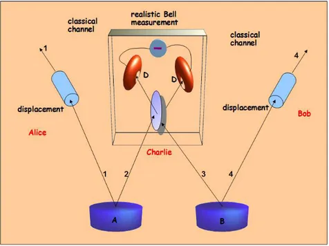
2.1 (Color online) Schematic picture of the non-ideal cv entanglement swapping protocol, in which two indipendent couples, A and B, of two-mode entanlged states (1− 2 shared by Alice and Charlie, 3− 4 shared by Bob and Charlie) are used for producing the final swapped entangled state (composed by 1 and 4 modes), shared by the two final users Alice and Bob. See text for more details. . . . 39 2.2 Pictorial representation (color online) of the scenario describing
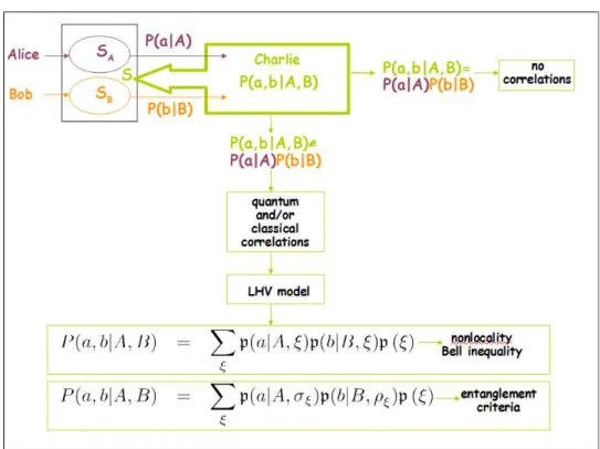
two possible test of nonlocality: Bell inequality and entanglement criteria. Alice makes a measurement on the subystem SA, while
Bob, indipendently, realizes a measurement on the subystem SB.
Charlie is the only acting on the joint system S. He compares the quantum expectation value (obtained considering whole system) with the product of the Alice’s and Bob’s results. If there isn’t coincidence the system is correlated. To discriminate the quan-tum correlations from the classical ones Charlie applies the hidden variables theory LHV. For more details see text. . . 40 2.3 Pictorial representation (color online) of the scenario describing a
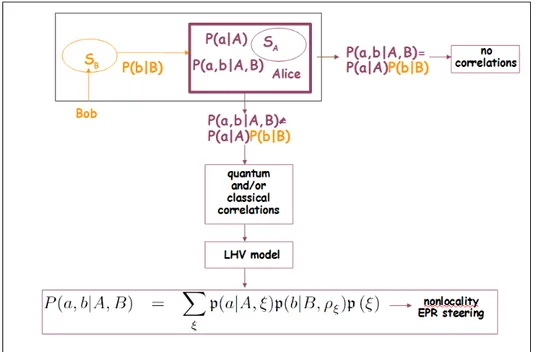
possible test of nonlocality: EPR-steering. Alice prepares the whole bipartite state. Then she gives the subpart SB to Bob. If two
sub-systems are correlated, then Alice can infer the Bob’s quantum
state by measurements made on SA. To discriminate the
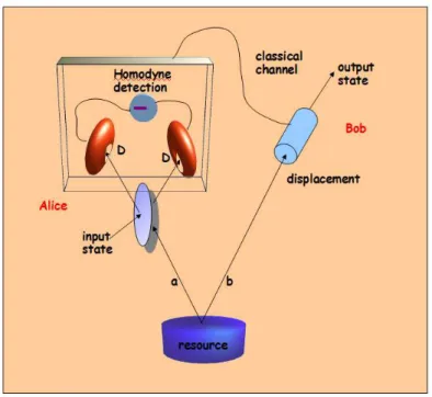
quan-tum correlations from the classical ones Alice applies the hidden variables theory LHV. For more details see text. . . 41 2.4 Schematic picture (color online) of the teleportation protocol, in
which the resource (a two-mode entanlged state a-b), shared by Alice and Bob, is used for teleporting the input state from Alice’s position to Bob’s position. See text for more details. . . 42 3.1 Region plot (color online) of the different entaglement witnesses
of Eqs. (3.12) and teleportation fidelity (Eq. (3.21)) as an entan-glement marker. The light gray (labelled with (VI)) areas indicate un-physical CMs (i.e. violating inequality (1.16). The different criteria show different regions of entanglement (see text for details). 51 3.2 (color online) Block diagram of the experimental setup, able to
implement the Eq. (3.23). The details on the OPO source are given §3.5.1 [54], while the characterization stage, based on a single homodyne detector, is fully described in Ref. [56, 58]. . . 55
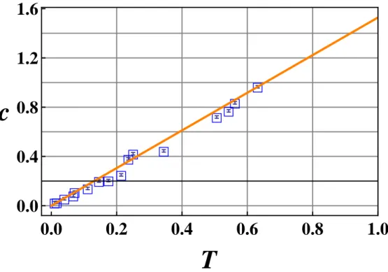
LIST OF FIGURES viii 3.3 (color online) Behavior of c =|c1,T|+|c2,T| /2 in Eq. (3.24). The full
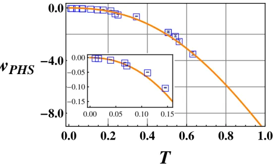
(dark orange) line represents the theoretical behaviour calculated starting from the first experimental point we have measured (T = 0.63); the experimental points (blue color) follow the theoretical line, i.e., as expected, the correlation reduces linearly with T . . . . 57 3.4 (color online) wP HS vs.T . The full (dark orange) line represents the
theoretical behavior, calculated starting from the first experimen-tal point at T = 0.63. Error bars are obtained by propagating the experimental uncertainty on the CM elements in the expression of wP HS in Eq. (3.12). The inset is a magnification of the plot in the
high loss regime (T < 0.15). We see that the un—separability per-sists, as witnessed by wP HS, even in presence of strong decoherence. 58
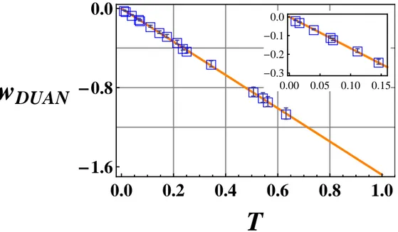
3.5 (color online) wDU AN vs.T . The full (dark orange) line represents
the expected behavior calculated starting from the first experimen-tal point we have measured (T = 0.63). Error bars on the exper-imental points (blue) are obtained by propagating the uncertainty on the measured CM elements in Eq. (3.12). The inset is a mag-nification of the plot in the high loss regime (T < 0.15) in order to stress the persistence of entanglement, as witnessed by wDU AN,
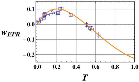
even in presence of strong decoherence. . . 59 3.6 (color online) wEP R vs.T . The full (dark orange) line represents the
expected behaviour calculated starting from the first experimental point we have measured (T = 0.63). Error bars are obtained by propagating the uncertainty on the CM elements in Eq. (3.12). They are considerably larger for point at low loss. . . 60 3.7 (color online) F vs.T . The full (dark orange) line represents the
expected behavior calculated starting from the first experimental point we have measured (T = 0.63). The inset is a magnification of the plot in the high loss regime (T < 0.15) in order to underline the persistence of a quantum teleportation regime even in presence of strong decoherence (high loss). . . 61 3.8 (color online) I and D vs.T . The full (dark orange) and dashed
(blue) lines represent the expected behaviors calculated starting from the first experimental point we have measured (T = 0.63) for I and D respectively. The inset is a magnification of the plot of D in the high loss regime (T < 0.15). We note the persistence of a true quantum correlation even in presence of strong decoherence (high loss). . . 62
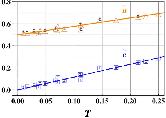
LIST OF FIGURES ix 3.9 (color online) Behaviour of the averaged correlation term |c1,T| +
|c2,T| /2 and of the averaged diagonal element nT = (nT + mT) /2
in Eq. (3.24). As expected the first reduces linearly with T . The straight (full and dashed) lines represent the expected behaviours calculated setting the less absorbed CM as the reference state. Error bars are smaller than data points and amount to ±0.01. . . 64 3.10 (color online) wP HSand wDU AN vs. T . The full dark orange (lower)
and the blue (upper) lines represent the expected behaviour of wP HS
and wDU AN respectively. Error bars range between 10−4 and 0.1. . 65
3.11 (color online) F vs. T . The full (dark orange) line represents the expected behaviour. Error bars, obtained by propagating the experimental indeterminacies in Eq. (3.21), range between 10−5
and 0.01. It si worth noting that even for T = 0.99 the experimental point lies inside the quantum region (F = 0.5023 ± .0.0002). . . . 66 3.12 (color online) I and D vs.T . The full (dark orange) and dashed
(blue) lines represent the respective expected behaviours. Error bars respectively, range between 3× 10⁻³ and 0.02 for I and 10−4
and 0.03 for D. Note that the data for I scatters more from the expected behaviour may be signalling extra classical correlations. 67 4.1 (color online) Behaviour ofBpureI as a function of wDU AN,
through-out the range of values identified by the codomain [−1, 0] of wDU AN. 71
4.2 (color online) Region plot of different nonlocality markers. The region I includes not entangled states, identified by the condition µs< µD; the region II includes entangled states that are local for
Bell (2.35), identified by the condition µD < µs < µB; The region III represents the entangled states that are also nonlocal, bordered by µB < µs < µF. See text for more details . . . 73
4.3 (color online) Behaviour ofBI as a function of transmission coeffi-cient T, simulanting decoherence. We note that decoherence heavily affecst the Bell’s nonlocality. In fact BI violates Bell’s inequality for a very little range of values of T . . . 74 5.1 (color online)−Plot of the Bell function for the optimized state
(blue solid line), for the P S state (green dot-dashed line), for the T B state (orange dashed line), and for the P A state (purple dotted line) for r ranging from 0 to 2. The inset is a magnification of the trends for r ∈ [0.2, 1.0]. . . . 81
LIST OF FIGURES x 6.1 (Color online) Optimized fidelity of teleportationFA(opt)swT B with A =
SB (full line), P S (dashed line), and T B (dotted line), as a func-tion of the squeezing parameter r12of the swapped input state, and
at fixed r34 = 1.5 of the swapping T B resource. For comparison,
we also report the plots of the teleportation fidelities associated with the corresponding non-swapped resources (same plot style, but with tinier and lighter lines). While the fidelities associated with non-swapped resources saturate to one, the fidelities associ-ated with swapped resources saturate to a lower level, depending on the swapping squeezing parameter r34. . . 87
6.2 (Color online) Relative teleportation fidelities ∆FSB(BswswT B)T B with B =
T B (full line) and B = P S (dashed line), as a function of the squeezing parameter r12 of the swapped input state, and at fixed
r34= 1.5 of the swapping TB resource. For comparison, we also
re-port the relative fidelities ∆FSB(A) associated with the corresponding
non-swapped resources (same plot style, but with tinier and lighter lines). . . 89 6.3 (Color online) Three-dimensional relative teleportation fidelity ∆FSB(T BswswT BT B)
as a function of the squeezing parameter r12 of the swapped input
resource, and of the squeezing parameter r34 of the swapping TB
resource. ∆FSB(T BswswT BT B) is monotone in r12 and r34. . . 90
6.4 (Color online) Three-dimensional relative teleportation fidelity ∆FSB(P SswswT BT B)
as a function of the squeezing parameter r12 of the swapped input
resource, and of the squeezing parameter r34 of the swapping TB
resource. . . 91 6.5 (Color online) Optimized fidelity of teleportationFA(opt)swA with A =
SB (full line) A = P S (dashed line) and A = T B (dotted line), as a function of the squeezing parameter r12of the swapped input state,
and at fixed r34 = 1.5 of the swapping resource. For comparison,
we also report the plots of the teleportation fidelities associated with the corresponding non-swapped resources (same plot style, but with tinier and lighter lines). The swapped SB resources show a sensibly higher saturation level with respect to the swapped PS and TB resources. . . 91 6.6 (Color online) Relative teleportation fidelities ∆FSB(AswswA)SB with A =
T B (full line) and A = P S (dashed line), as a function of the squeezing parameter r12 of the swapped input state, and at fixed
r34 = 1.5 of the swapping resource. ∆F(P S
swP S)
SBswSB never vanishes for
LIST OF FIGURES xi 6.7 (Color online) Optimized fidelity of teleportation FA(opt)swB with A =
B = SB (full line), A = B = P S (dashed line), A = SB, B = T B (dot dashed line), A = P S, B = T B (double-dot dashed line), and A = B = T B (dotted line), as a function of the squeezing para-meter r12 of the swapped input state, and at fixed r34= 1.5 of the
swapping resource. The parameters of the experimental apparatus are fixed as: τ1 = 0.1, nth,1 = 0, τ4 = 0.2, nth,4 = 0, R2 =
√ 0.05, R3 =
√
0.05. The swapped SB resources show a sensibly higher saturation level with respect to the swapped P S and T B resources. 92 6.8 (Color online) Relative teleportation fidelities ∆FSB(BswswC)A with A =
SB, B = C = P S (full line), A = SB, B = C = T B (dotted line), A = C = T B, B = P S (dashed line), A = B = C = T B (dot-dashed line), as a function of the squeezing parameter r12 of
the swapped input state, and at fixed r34 = 1.5 of the swapping
resource. The parameters of the experimental apparatus are fixed as in Fig. 6.7. . . 93 7.1 (Color online) the block-scheme of ideal setup for generating the
class of states Eq. (7.4). Two indipendent twin beam |ζ 12 and |ξ 34, are mixed into two beam splitters BSI and BSII of
transmit-tivity T1 and T2, respectively. Two single photon detectors D3 and
D4 realize simultaneous ddetections. . . 95
7.2 Realistic scheme (color online).(color online). At the ideal scheme (Fig. (7.1)), four fictitious beam splitters of transmittivity Tℓare
in-troduced to mimic dechoerence mechanisms. Moreover, the single-photon detectors are replaced by POVMs (Π(on)3 and Π(on)4 ) with quantum efficiencies η < 1. . . 100 7.3 (Color on line) Fidelity of teleportation of the state generated from
our scheme in the ideal instance (single-photon conditional mea-surements) plotted vs. the ancillary squeezing parameter s (≤ r) for different values of the main squeezing parameter r: (a) r = 0.6 (brown full line); (b) r = 0.8 (purple dashed line); (c) r = 1 (red large—dashed line); (d) r = 1.2 (blue dotted line); (e) r = 1.4 (green large—dotted line); (f) r = 1.6 (black dotted—dashed line); (g) r = 1.8 (magenta double dotted—dashed line); (h) r = 2 (or-ange triple dotted—dashed line). The point at s = 0 corresponds to the fidelity achieved with a PS squezed state generated in ideal conditions, while at s = r we obtain the fidelity achieved with a TB, generated as well in ideal conditions. . . 105
LIST OF FIGURES xii 7.4 (Color online) Comparison among: the optimized fidelity on the
class of generated states in the ideal instance of generation (red dashed), the fidelity of the PS squeezed state generated in the ideal instance (green large—dashed), the optimized fidelity of the theo-retical SB states (cyan continuous), the fidelity of the theotheo-retical PS squeezed states (purple dotted—dashed), and the fidelity of the theoretical TB (black dotted). . . 107 7.5 (Color online) Details of Fig. 7.4 in the range 1≤ r ≤ 2 for: the
op-timized fidelity on the class of generated states in the ideal instance of generation (red dashed), the fidelity of the PS squeezed state generated in the ideal instance (green large—dashed), the optimized fidelity of the theoretical SB states (cyan continuous) the fidelity of the theoretical PS squeezed states (purple dotted—dashed), and the fidelity of the theoretical TB (black dotted). . . 108 7.6 (Color online) Fidelity of teleportation in a realistic lossy scenario
(level of losses equal to 0.15, i. e. Tℓ = 0.85, and η = 0.15). The
fidelity depends on the squeezing parameters s, r, and has been plotted vs. s (≤ r) for the same values of r used in Fig. 7.3: (a) r = 0.6 (brown full line); (b) r = 0.8 (purple dashed line); (c) r = 1 (red large—dashed line); (d) r = 1.2 (blue dotted line); (e) r = 1.4 (green large—dotted line); (f) r = 1.6 (black dotted—dashed line); (g) r = 1.8 (magenta double dotted—dashed line); (h) r = 2 (orange triple dotted—dashed line). . . 109 7.7 (Color online) Optimized fidelity of the states generated in realistic
conditions (with η = 0.15) plotted as a function of the loss parame-ter ℓ, for r = 1.6 (blue full line). The plot is compared with those relative to the fidelity of the PS squezed states (s = 0, dark line)) and to the fidelity of the TB (s = r, green large—dashed line), when both are generated in realistic conditions with η = 0.15. . . 110
Part I
Preamble
0.1. INTRODUCTION xiv
0.1 Introduction
It is now ascertained that quantum mechanics is a powerful tool in the In-formation and Communication theory. The quantum properties of light radiation allow to implement, relatively easily and with high efficiency, large part of Quan-tum Information protocols, developed to make possible the transfer of information to a point arbitrarily far away. Many of the properties, which make the quantum theory an instrument so precious, are related to the linear nature of the theory. It is this linear nature the main cause of the existence of most of the quantum paradoxes, included the celebrated EPR paradox. As is well known, this paradox arises, in 1935, with the interrogative-paper [1] of Einstein-Podolsky and Rosen EPR Can Quantum-Mechanical Description of Physical Reality Be Considered Complete? Authors’ aim was to demonstrate the incompleteness of Quantum Theory. The scientific history of the last seventy-eight years shows that EPR did not reach their goal, but they paved the way for the discovery of genuinely quan-tum correlations, which Schrodinger [2] called entanglement. Such correlations are the basis of most efficient protocols developed to date in the field of quantum mechanics. An entangled state is such that it cannot be factorized into pure local states of which it is composed. This is because the subsystems share quantum correlations. The Quantum Information theory exploits such nonclassical corre-lations to encode, to process and to distribute information by techniques that are impossible to implement, or that give very inefficient results, in the context of classical physics. For this reason, in the last decades, many efforts have been aimed at the production of entangled quantum states and at the study of the quantum properties that take a quantum state to become a efficient resource in the Quantum Information protocols. What is the best quantum resource to use depends on the protocol that we choose and on the purpose we want to achieve.
A protocol widely studied in Quantum Information is arguably the quantum teleportation. As is known, the no-cloning theorem, which is a direct consequence of the postulates of quantum mechanics, forbids, in agreement with the theorem of quantum non-discrimination, to create an exact duplicate of an unknown quan-tum state. However, it is possible to transfer the quanquan-tum state from a system to another system, provided, of course, the no-cloning theorem is respected.This im-plies that the information in the original system must be destroyed. The quantum teleportation is a technique that allows, under certain restrictions, to transfer a quantum state from one system to another one arbitrarily far away. This protocol is based on the fact that the two parts, called Alice and Bob, between which it must take place the transfer of the state, share an entangled state, that is the resource of the protocol.
Quantum states can be divided into two main categories: Gaussian states and non-Gaussian states. The state describing a system belongs to one either category depending on the statistical distribution of the observable of the state. Gaussian states play an exceptional role in Quantum Information theory. They are easy to
0.1. INTRODUCTION xv produce and control in the laboratory. Indeed they can be obtained in nonlinear processes such as parametric amplifiers, in which a nonlinear medium is allocated in an optical cavity providing an optical parametric oscillator OPO. Such systems, in a semiclassical approach, are described by bilinear Hamiltonians, thus realize the paradigm for the Gaussian state generation. In particular, below threshold a single continuous-wave OPO, generating squeezing in a fully degenerate operation can give rise to a pair of bright cv entangled beams in the nondegenerate case. It leads to states that represent robust resources for implementing different Quantum Information and Communication tasks. These states, however, also suffer from some limitations, both technical (which occurs if we try to generate states with very high degree of entanglement) and intrinsic properties of the quantum theory (Extremality of Gaussian Quantum States [3]). In this context, a appropriately sculptured non-Gaussianity can become a resource for the efficient implementa-tion of the quantum protocols. All quantum states that can not be described by a Gaussian distribution function are non-Gaussian states. To identify the special features that bring a non-Gaussianity to be a resource in Quantum Information is not easy. In recent years many efforts have been made in the analysis of quantum properties of classes of non-Gaussian states and in the engineering of experimental schemes, making it possible to easily prepare and control non-Gaussian states in the laboratory. Many advances have been made both in terms of experimental and theoretical aspects. In the theoretical framework the features, whose must enjoy a quantum state to be an optimal resource of quantum teleportation, have been identified [4], in the context of continuous variables. A new class of states, the Squeezed Bell states [4], has been proposed. It is able to offer a probability of success of the teleportation protocol BKV greater than that provided by the main known Gaussian and non-Gaussian resources [4], [5]. In the experimental framework, some non-Gaussian quantum states have been implemented and, in parallel, some techniques which avoid the use of optical active means (such the OPO) have been developed. The crucial point of the experimental reality, at least with regard to the continuous variables cv quantum optics, is the impossibility to produce, realistically speaking, pure states. This occurrence leads to the new interpretations of many physical concepts and opens many questions in Quantum Information. For example, the definition of an entangled state is conceptually connected to pure states. The properties of these states are described by wave functions. All the gedanken experiments that we can think to realize for testing the different theoretical aspects of the entanglement lead to a same entanglement measure, but the pure entangled states, discussed in such experiments, are an idealization. The states we can prepare and manipulate in the laboratory are not pure but mixed, so we cannot expect to observe precisely the phenomenon intro-duced by the theory. The experimental entanglement tests, especially in the cv regime, are described in terms of density matrices rather than wave functions. It is necessary becouse the systems interact with the environment and/or observers,
0.1. INTRODUCTION xvi therefore they undergo decoherence phenomena departing far from the ideal con-cept of pure states. In optics the most common process leading to decoherence is the phase-insensitive loss of photons through diffusion and absorption mecha-nisms. This process is described by a Lindblad equation for the evolution of the field operators that translates into a Master equation for the state density matrix. This Dissertation collects my personal both theoretical and experimental con-tributions, in the context of the Quantum Information theory and, more generally, of the Quantum Optics in continuous variables. In this context, I have dealt with various issues related to the efficiency of realization of quantum information pro-tocols. Much of the research has been aimed at identifying the resources that allow to realize quantum teleportation with a highest probability of success. For this reason we proceeded to the study of quantum quantities that influence the success rate of teleportation of a quantum state, in the protocol BKV.
The quantum resources, as we said so far, can be divided in two main classes: Gaussian resources and non-Gaussian ones. My research activity has been struc-tured in which way to be able to proceed, in parallel, to the analysis of both classes.
This Dissertation is organized as follows.
After describing some basic concepts of the quantum theory (chapter 1) in order to clarify the context in which it was carried out the results of the re-search, in the chapter 2 we explore the concept of quantum state as resource. We investigate the properties that allow to distinguish between classical states and non-classical ones (§ 2.1). Then we analyze, in more detail, the features that define the quantumness of a state as, for example, the mutual information (§ 2.2) and the quantum discord (§ 2.3). We clarify the difference between entanglement measure and entanglement criteria. Then we describe, in the formalism of the characteristic function, the protocol of entanglement swapping, through which it is possible to transfer the entanglement from two couples of entangled modes to one couple of unentangled modes. Quantumness and nonlocality are two closely related concepts. So we try to clarify some aspects of this relationship. We com-plete the chapter with a description of the protocol of quantum teleportation. In the first two chapters we lay the foundations in order to proceed to the description of the original findings. We can divide such description into two main parts.
The first part (chapters 3 and 4) is dedicated to the results carried out on the pure and mixed Gaussian resources.
To date there isn’t a single measure that quantifies the entanglement of mixed states and various measures have been suggested in the literature, they are not easy to apply and provide sometimes conflicting results. To assess the presence of entanglement in a quantum system it is possible to refer to the many crite-ria proposed in the literature. The critecrite-ria are often the most used tool, in the experimental Quantum Optics field, to evaluate the quality of entanglement of a
0.1. INTRODUCTION xvii quantum-optical system. In chapter 3 we study some of the main criteria generally used for Gaussian bipartite mixed states. This study has allowed us to establish a hierarchy very useful for the evaluation of the entanglement [6]. Then we have discussed and experimentally analyzed the effects of the transmission over a lossy channel on the quantumness of bipartite Gaussian cv optical entangled states, focusing our analysis on the states generated by a type-II OPO [7]. The obtained results are reported in [6], [8]. Eventually, in chapter 4, it is reported the study of the Bell’s inequality in terms of purity and entanglement for a bipartite Gaussian state. The need to begin such a study comes two considerations: the deterio-ration of the purity of a quantum state greatly affects the performance of the system associated with that state; the entanglement is not the only type of gen-uinely quantum correlation present in quantum systems. It becomes necessary, therefore, to investigate how the "quantumness" owned by a state, established by the violation of Bell’s inequality, is related to the purity of the state and to the entanglement. The obtained results are reported in [9].
The second part (chapters 5, 6, 7 and 8) is dedicated to the results carried out on non-Gaussian resources. The study of non-Gaussian resources mainly related to a particular class of states: the squeezed Bell states. All the analysis carried out to date show that these states are one of the best possible resources for efficient cv quantum teleportation protocol BKV. We proceed as described below. In order to assess which quantum resource allows to have a higher probability of success in the quantum teleportation of a coherent state, have processed the following two theoretical tests:
1. In chapter 5 we report the study of the behavior of the Bell’s inequality for the whole class of states obtained by the squeezed Bell states. Such study makes possible to determine what is the quantum resource that maximizes the violation of the inequality, i.e. which is the most "non-local resource" among all those considered. The results are collected in a paper of next submission [10].
2. In the chapter 6, we analyze the performances of teleportation provided by Bell squeezed resource, when it is subjected to two cascade protocols: at first the squeezed Bell undergoes a swapping process; then the swapped state is used as resource in a quantum teleportation protocol. The result is compared with that provided by the other main quantum swapped resources. The results are collected in a paper of next submission [11].
to understand how a resource behaves after undergoing a process of swapping is very useful becouse error probability, in a transmission channel, scales with the length of the channel. However it is possible to divide the channel into segments of shorter length and applying a protocol of entanglement swapping to restore the lost entanglement. This test is particularly useful to reconfirm
0.1. INTRODUCTION xviii the squeezed Bell states as one of the best resources suitable in quentum Information, implemented within quantum theory quantum information. As a consequence of the positive results of the two studies conducted to in-vestigate the "quantum qualities" of the class of the squeezed Bell states, we have proceeded (chapter 7) to the design of an experimental scheme of engineering, that is capable to produce bimodal state, similar to squeezed Bell one. The analysis of the ideal scheme has been expanded to the realistic case by introducing all pos-sible contributions of losses, decoherence effects and detection for evaluating the actual "experimental feasibility" of the sculptured resource and to provide, with good approximation, the desired squeezed Bell state.The results are reported in a paper of next submission [12].
In the chapter 8 it is reported the study of different types of non-Gaussian states. In fact, the investigation of the technical limitations, that afflict the OPOs sources, for the generation of Gaussian states with a high degree of entanglement, has allowed us to understand that these "inconveniences", under appropriate con-ditions, can become a resource for the generation of non-Gaussian states . These considerations have led to the study of non-Gaussianity produced by fluctuations of pump beam in a sub-threshold OPO. We have assumed to use this particular non-Gaussian state as a resource for the teleportation of a coherent state. The obtained fidelity, i.e. the probability of success of the teleportation, is greater than that of a Gaussian resource. This result has allowed to discover a new type of non-Gaussian resource, capable of realizing quantum teleportation with a high probability of success.
CHAPTER 1
PRELIMINARIES
In a outlook, that can be called positivistic, because it coincides with the attitude at first adopted by logical positivists, we can divide any physical theory into the following constituents: (a) the formalism, expressed in terms of primitive con-cepts; (b) the rules of deduction, enabling us to derive theorems by manipulating the symbols associated to the formalism; (c) the dynamical law, imposing addi-tional restrictions on values which can be taken by some primitive concepts; (d) the correspondence rules, establishing the link between experience and theory [13]. In this chapter, we present some of these constituents in the context of the Quantum Theory. They are preliminaries and allow us to introduce concepts as continuous variables (see § 1.1.1), pure and mixed states (§ 1.1.2), Gaussian and non-Gaussian states (in § 1.1.2.1 and 1.1.2.2), and notations that will be frequently used throughout the Dissertation.
1.1 Observables and States
In this section we introduce the primitive quantum concepts of observable and state, by establishing the link between the mathematical formalism and the physical meaning [14].
1.1.1 Observables
An observable is rappresented by a self-adjoint operator on a Hilbert space with spectral representation
O =
n
onPn,
where Pn are orthogonal projectors of O,
Pn= a
|a, on a, on| ,
with on eigenvalues of O and the parameter a labels the degenerate eigenvectors
belonging to the same eigenvalue of O. An observable has a complete orthogonal set of eigenvectors. An observable is a theoretical construct, whose domain of definition is a subset of a set of the real numbers, called spectrum of the observable, and which is associated, by means of given correspondence rules, with one or more measurable quantities.
The sums become integrals in the case of continuous spectra. 1
1.1. OBSERVABLES AND STATES 2 So the observables of quantum systems can posses either a discrete or a con-tinuous spectra. The quantum electromagnetic fields have both the concon-tinuous and discrete degrees of freedom. For example, the photon number of the field gives discrete outcomes whereas measurements of the field’s quadrature provide continuous outcomes. A physical model that takes advantage of both the degrees of freedom is called hybrid. In this dissertation we’ll refers mainly to the continuos degrees of freedom of the quantum electromagnetic field.
1.1.2 The quantum state
The state of a physical system is the mathematical description of the knowl-edge one has of it. It is represented by a self-adjoint, non-negative definite, and of unit trace operator. This implies that any state operator, called also density matrix ρ, may be diagonalized in terms of its eingenvalues and eigenvectors,
ρ =
n
ρn|φn φn| , (1.1)
with 0 ≤ ρn ≤ 1 and nρn = 1. For a pure state, the statistical operator ρ is idempotent, ρ2 = ρ, so there is exactly one non zero eigenvalue of ρ, i. e. ρ
n= 1,
ρn′ = 0 for n = n′. A pure state may be represented by wave vector |φ in the
Hilbert space such as ρ = |φ φ| . A generic state, which is not pure, is called mixed. Density matrix formalism encopasses the possibility of describing both pure and mixed states. In this context it becomes very important to introduce the parameter purity µ,
µ = T r[ρ2], (1.2)
such as
1
N ≤ µ ≤ 1 (1.3)
with N dimension of the Hilbert space, µ = 1 only for pure states. In the context of the continuous variables 0 ≤ µ ≤ 1. The purity assumes a relevant role in quantum information protocols, indeed the fidelity, i.e. the rate of success of the protocol, depends critically on the purity of the all involved states.
An description, alternative to operatorial one, of the state is given in terms of the characteristic function χ(λ) = T r[ρD(λ)], where D(λ) is the displacement operator, that for n bosons is defined by
D(λ) =
n
k=1
Dk(λk),
where λ is the column vector λ = (λ1, ..., λn)T, λk ∈ C, k = 1, ..., n and Dk(λk) =
1.1. OBSERVABLES AND STATES 3 The characteristic function is also known as the moment-generating function, since its derivatives in the origin of the complex plane generate symmetrically ordered moments of the mode operators,
(−)q ∂p+q
∂λpk∂λ∗pl χ(λ)λ=0
= T r[ρ[(a†k)paql]S], (1.4)
where, for the first non trivial moments we have a†a S = 1 2(a†a + aa†), aa†2 S = 1 3(a†2a + aa†2+ a†aa†), a†a 2 S = 1 3(a 2a†+ a†a2+ a†a) [15].
The Fourier transform of the characteristic function is called Wigner distrib-ution, W (α) = Cn d2nλ π2n exp{λ †α+ α†λ}χ(λ). (1.5)
1.1.2.1 Bipartite Gaussian State
A continuous-variable Gaussian bipartite state ρab is two-mode state, on the
Hilbert space H = Ha ⊗ Hb, that has a representation in terms of Gaussian
characteristic function or, equivalently, Gaussian Wigner function
W (K) = exp{−
1 2K
Tσ−1K}
2π Det[σ]
where σ is the covariance matrix and K≡ (Xa, Ya, Xb, Yb) is the vector of the
amplitude and phase field quadratures for mode a and b respectively. We have considered null the first moments. In quantum optics, the quadrature operator assumes the role of the dimensionless variables position q and momentum p. It is defined as follow:
Xϑ≡
aeiϑ+ a†e−iϑ
√
2 . (1.6)
For ϑ = 0, X0 = X, called amplitude quadrature, is identical to adimensional
position operator q, whereas, for ϑ = π/2, Xπ/2 = Y , called phase quadrature, is
identical to the adimensional momentum operator p. From commutation relation ak, a†l = δkl results that [X, Y ] = i.
All the quantum features of a Gaussian state can be retrieved experimentally by measuring the first and second order statistical momenta of the field quadra-tures, i.e. the covariance matrix (CM) σ
σ = α γ
γ⊤ β , (1.7)
with elements σhk ≡ 12 {Kk, Kh} − Kk Kh , where{Kk, Kh} ≡ KkKh+ KhKk
1.1. OBSERVABLES AND STATES 4 reduced state of the subsystems a and b, while γ describes the correlation between the two subsystems. For this reason they are of great practical relevance, being feasible to produce and control with linear optical elements. Moreover this state appears naturally in every quantum system which can be described or approxi-mated by a quadratic Bosonic Hamiltonian. Important examples include vacua, coherent, squeezed, thermal, and squeezed-thermal states of the electromagnetic field.
To study the correlation between the two modes of the system it is convenient, at first, to transform the Gaussian state into some standard forms through local symplectic operations, that is transformations preserving canonical commutation relations of the quadratures. Any Gaussian state ρG can be trasformed, through symplectic transformations, into the standard form
σ = n 0 c1 0 0 n 0 c2 c1 0 m 0 0 c2 0 m . (1.8)
The quantities n, m, c1 and c2 are determined by the four local symplectic
invari-ants I1 ≡ det(α) = n2, I2 ≡ det(β) = m2, I3 ≡ det(γ) = c1c2, I4 ≡ det(σ) =
(nm− c2
1) (nm− c22). Hereafter, whenever we refer to CM we will intend the
standard form covariance matrix (1.8) if not differently specified. As we men-tioned above the purity of the state, and so also the condition Eq.(1.3), becomes a essential constraint to establish the physicity of the state under investigation.
For a Gaussian state Eq. (1.2) reads
µ (σ) = 1
4 Det [σ]. (1.9)
From Eq. (1.3) we obtain the following constraint on the symplectic invariant I4:
I4 ≥
1
4. (1.10)
1.1.2.2 Non-Gaussian States
All states that do not have a Gaussian Wigner function are called non-Gaussian nG states. As we will see in the following of Dissertation, non-Gaussianity is re-vealing itself as a resource for continuous variable Quantum Information. For this reason there needs a measure able to quantify the non-Gaussian character of a quantum state.
Departures from Gaussian statistics may be noted by the observation of the higher moments than the second one. It is possible, for example, to measure the kurtosis, i. e. the fourth moment X4 and to evaluate the kurtosys excess
1.1. OBSERVABLES AND STATES 5 K = XX2 24 − 3. The "minus 3", at the end of this formula, is added as a
cor-rection to make the kurtosis of the normal distribution equal to zero, so K is zero for a Gaussian random variable, while for most (but not all) non-Gaussian random variables it takes values different from zero. Moreover, random variables with negative kurtosis are called sub-Gaussian variables, while random variables with positive kurtosis are called super-Gaussian variables. Unfortunately, to use kurtosis as nG measure presents some drawbacks. Indeed, although it is easy to evaluate by a known probability density function, it becomes more complicated to estimate it by a measured sample, becouse kurtosys may strongly depend on only a few observations in the tails of the distribution. For this reason K is not considered a robust measure of nG [16].
Different nG measures have been proposed to quantify the non-Gaussian char-acter of a state, as the Hilbert-Schmidt distance DHS and the quantum relative
entropy S. Although DHS and S are based on different quantities, they share the
same basic idea: to quantify the nG of a state ρNG in terms of its distinguishability from a reference Gaussian state τ , where τ is chosen in which way that it exhibits the same covariance matrix and the same vector K of the non-Gaussian state ρN G[16]. In the following we describe the main measures, introduced in leterature [17] ,[16], for evaluating the non-Gaussianity of ρNG:
nG using Hilbert-Schmidt distance [17]. Let δHS[ρNG]≡
D2HS[ρNG, τ ]
µ (ρN G) , (1.11)
with D2
HS[ρNG, τ ] the Hilbert distance between ρNG and τ ,
D2HS[ρNG, τ ] = 1 2T r (ρN G− τ) 2 = µ (ρNG) + µ (τ )− 2κ [ρNG, τ ] 2 ,
where µ denotes the purity of the corresponding state and κ [ρN G, τ ] is the overlap between ρNG and τ , κ [ρNG, τ ] = T r[ρNGτ ].
nG using quantum relative entropy. Let
δS[ρNG]≡ S(ρNG||τ) = T r[ρNGln ρNG]− T r[ρNGln τ ] = S(τ )− S(ρNG), (1.12)
where S(ρNG||τ) ≡ T r[ρNG(ln ρNG − ln τ] is the quantum relative entropy, i. e.
the quantum entropy relative to the Gaussian reference τ , and S(ρ) is the von Neumann entropy of the state ρ, S(ρ) =−T rS[ρSLogρS].
Although the two measures δHS[ρNG] and δS[ρNG] capture, in general, the
same qualitative non-Gaussian behavior [16], they induce different ordering on the set of quantum states; that is, it is possible to obtain δHS[ρNG1] > δHS[ρN G2] and
δS[ρNG1] < δS[ρNG2], or viceversa, with ρNG1and ρNG2two different non-Gaussian
states. This is probably due to the fact that different measures correspond to dif-ferent operational meanings of non-Gaussianity: δHS takes in account the higher
1.2. DYNAMICAL LAW 6 moments of the distribution, while δS is based upon the fact that Gaussian
dis-tributions maximize the von Neumann entropy at fixed covariance matrix. However, the two measures are connected one to each other by means of the inequality S(ρNG||τ) ≥ D2
HS[ρNG, τ ], i.e. δS[ρN G] ≥ δHS[ρNG1]µ (ρNG), that for
pure states becomes δS[ρNG]≥ δHS[ρNG1].
1.2 Dynamical law
In this Section we review the suitable formalism [18], [19] to describe the transmission of an arbitrary quantum state between regions spatially separated.
Any physical operation that reflects the time evolution of the state of a quan-tum system can be regarded as a channel. In particular, the study of quanquan-tum channels is useful to understand how quantum states are modified when subjected to noisy quantum communication lines.
The evolution of an arbitrary two-mode state is an irreversible process, the study of which requires the use of the open systems theory. In this context, we can postulate an weak coupling gj of the considered system S with a reservoir
(bath) R made of large number of external modes. In particular we assume: ◦ Born approximation - the coupling between system and environment is so weak that the density matrix ρR of the environment is negligibly influenced by the interaction. This approximation allows to write the state ρSR(t) of the global
system as ρSR(t)≈ ρS(t)⊗ ρR;
◦ Markov approximation - the time development of the state of the system at time t only depends on the present state ρS(t). This approximation is justified
if the time scale τ over which ρS(t) varies appreciably under the influence of the bath is large compared to the time scale τRover which the bath forgets about its
past, τ ≫ τR.
◦ Secular approximation (rotating wave approximation)- the typical time scale τS of the intrinsic evolution of the system S is small compared to the relaxation
time τ .
These assumptions are typically satisfied for quantum optical systems and allow to obtain the equation of the Kossakowski-Lindblad, that describes the time evolution in noisy channel of the bipartite quantum state ρS in the interaction
picture ˙ρS = k=1,2 Γk 2 (Nk+ 1)L [ak] + NkL a † k − Mk∗D [ak]− MkD a†k ρS ,
where Γk denotes the damping rate of the k−mode, Nk ∈ R and Mk ∈ C
are, respectively, the effective photons number and the squeezing parameter of the reservoir b. L [O] is the Lindblad superatoroperator defined by L [O] ρ ≡ 2OρO† − O†Oρ− ρO†O describing losses and linear, phase insensitive,
de-1.3. UNCERTAINTY PRICIPLE 7 pendent fluctuations. We have considered that each mode evolves independently in its channel and there aren’t correlations among noises in different channels.
In the chapter 3 we describe the our experimental implementation [6], [8] of a quantum channel. In such case, we had a thermal reservoir, i. e. Mk = 0. So,
at the room temperature, i. e. Nk ≃ 0, the evolution of system S is described by
the equation of motion
˙ρ =
k=1,2
Γk
2 L [ak] ρ, (1.13)
where Γkis the damping rate of the trasmission channel of the k−mode (k = 1, 2).
From now on, we consider that the damping rates don’t depend of the channel, Γk = Γ (for k = 1, 2).
In the formalism of the Wigner function Eq.(1.5), the Eq. (1.13) becomes the Fokker-Planck equation, ∂tW (R, t) = Γ 2 ∂ ⊤ RR+ 1 2∂ ⊤ R∂R W (R) (1.14) = Γ 2 ∂ ⊤ RR+ 1 2∇ 2 R W (R) , where ∂⊤ R = (∂X1, ∂Y1, ∂X2, ∂Y2) and ∇ 2 R= ∂R⊤∂R = ∂X2 1 + ∂ 2 Y1 + ∂ 2 X2 + ∂ 2 Y2.
1.3 Uncertainty priciple
Let A and B be two hermitian, not compatible operators, i.e such that their commutator is not null. The condition [A, B] = 0 prevents the two operators have simultaneous eigenvectors. However, we can estimate how much the eigenvector of A is far from that of B. When |ψ is eigenvector of A, the variance is zero, i.e. ψ| A2|ψ = ψ| A |ψ 2
. So the variance is a measure of how close we are to
an eigenvector. We can define the following operators: a ≡ ∆A = A − A and
b ≡ ∆B = B − B . They allow us to neglect the mean value without loss of
generality1,
∆J = 0
(∆J)2 = J2 − J 2 = j2 ,
with J = A, B and j = a, b. We obtain
∆A∆B ≡ ψ| A2|ψ ψ| B2|ψ
= Aψ|Aψ Bψ |Bψ
≥ | Aψ |Bψ | . 1the variances don’t change.
1.3. UNCERTAINTY PRICIPLE 8 In the last line, we have invoked the Cauchy-Schwarz inequality, in view of the which we obtain
∆A∆B ≥ | ψ| AB |ψ | .
Now, we consider the following operators O1 ≡ 12[a, b] and O2 ≡ 12{a, b}, where the
braces {...} refer to the anti-commutator. They are antihermitian and hermitian, respectively, O1 ≡ 1 2[a, b] =− 1 2(ba− ab) = − 1 2(ab) †− 1 2(ba) †=−O† 1, O2 ≡ 1 2{a, b} = O † 2,
so it is clear that the eigenvalue of O1+O2 = ab is the sums of an pure immaginary
number and pure real one. Since the magnitude of a complex number is greater than or equal to the magnitude of its imaginary part, we can write
(∆A)2 (∆B)2 ≥ 1
4 [A, B]
2
+ 1
4 {a, b} with {a, b} ≥ 0. From which we obtain the following inequality
(∆A)2 (∆B)2 ≥ 1
4 [A, B]
2
, (1.15)
that is the uncertainty Heisenberg’s principle. Physically realizable quantum states must comply with this inequality. It then provides information on the physicality of the analyzed quantum state.
We note that the inequality Eq.(1.15) was obtained for pure states [20],[21]. It has been demonstrated to be valid also for mixed states [22]. However, in the case of pure states it is able to provide useful informations about the nature of the state under consideration. For example it can be shown that the state that minimizes the uncertainty, i. e. the state in which the inequality Eq. (1.15) is verified with the sign of equality, has Gaussian distribution. For mixed states, however, the inequality is, in general, strongly violated, so that it is not possible to extract useful information on the distribution. Moreover, in the mixed state case, also the purity Eq.(1.3) contributes to the physicality.
We have seen that the uncertainty principle is a direct consequence of the com-mutation relations for non-compatible observables. As a consequence, the inequal-ity (1.15), applied to the quadrature operators, provides (∆X)2 (∆Y )2 ≥ 1
4.
Uncertainty relations among canonical operators impose a constraint on the covariance matrix, in according to which σ represents a physical state iff
σ+ i
1.3. UNCERTAINTY PRICIPLE 9
where Ω = ω ⊕ ω is the two-mode symplectic matrix, with ω ≡ 0 1
−1 0 .
Moreover the Heisemberg uncertainty (1.16) can be written in terms of the four symplectic invariants
I1+ I2+ 2I3 ≤ 4I4 +
1
4. (1.17)
The inequalities (1.16),( 1.17) ensure that σ is a bona fide CM, i. e. it describes a physical state.
However, every covariance matrix is, by definition, real symmetric positive definite. These information are stored in the constraints (1.16), (1.3), but not in the (1.17). Therefore, the use of (1.17) requires more caution. It alone does not ensure the physicality. It must be accompanied by the condition of positivity of the density matrix, expressed, for example, by (1.3).
1.3.1 Squeezed states
A state is squeezed in respect to the observable A if (∆A)2 < 1
2 [A, B] 2
. So the squeezing is the reduction of quantum fluctuations in one observable below the standard quantum limit (vacuum fluctuation) at the expense of an increased uncertainty of the conjugate variable.
Squeezed states are an example of advantageous interchange between exper-iment and theory in quantum optics. To be able to discuss the characteristics it is not possible don’t consider the process that generates them (described briefly in the following). The squeezed states are produced through a process of Optical Parametric Generation OPG, in which the pump beam (typically a laser beam, which emits radiation in the coherent state |β ), at the frequency ωp,impinges
on a not center-symmetric crystal. At the output of the non linear crystal two signals a and b are produced, such that the pump energy is distributed between two output,
ωp = ωa+ ωb,
and the total momentum is preserved. When the outputs a and b are degenerate in frequency (degenerate OPG), and with the same wave vectors, the interacting Hamiltonian reads
Hint= i |ςβ| [eiφa†b†− e−iφab], (1.18)
where we have considered the average on the input coherent state|β , φ = arg(β)+ arg(ς) and ς is the coupling parameter.
In according to Hamiltonian Hint Eq. (1.18) the pure two-mode squeezed
vacuum state reads
|ψ ab ≡ e
i
1.3. UNCERTAINTY PRICIPLE 10 We note that putting |ςβ| eiφt = reiφ ≡ ξ, with ξ = reiφ arbitrary complex
number, we obtain the expression of |ψ , Eq. (1.19), in terms of the squeezing operator S(ξ),
|ψ ab = S(ξ)|00 12, (1.20)
with S(ξ) = e12(ξ ∗
ab−ξa†b†)
. We note the module r of ξ is linked to the intensity of the pump laser beam and the phase φ is manipulable through delay lines, so the parameter of squeezing ξ is completely under experimental control.
Tipically modes a and b generated by an OPG are weak, for this reason the active medium (nonlinear crystal) is put often into an optical cavity. Under appro-priate conditions the parametric interaction can overcome the effects of possible losses (i.e. absorption, diffraction...). In this case the system undergoes an oscil-lation and intense output beams are obtained. Such a device is called an Optical Parametric Oscillator (OPO). The modes at the output of the OPO are ther-mal modes, but their linear combination is squeezed. We express the two-mode squeezing operator Sab(−r) in terms of single-mode squeezing operators Sc(r) ,
Sd(−r). These are obtained by introducing the annichilation operators ˆc and ˆd
made by the superpositions
ˆ c = ˆa + ˆb√ 2 , ˆ d = −ˆa + ˆb√ 2 . We have Sab(−r) |00 >ab= Sc(−r) Sd(r)|00 >cd, (1.21)
where ˆSk(ξ) = exp −12ξˆk†2+12ξ∗ˆk2 , (k = c, d) is the single-mode squeezing
op-erator. Consequently, the characteristic function that describes the state |ψ >cd
results
χcd(βc; βd) = Tr ρcdDˆc(αc) ˆDd(αd) ,
where ρcd =|ψ >cd cd< ψ|. We compute the variance of the modes c and d by the
characteristic function ( moment-generating function). Indeed, from the relation Eq. (1.4) we obtain the following variances
∆2Xc = ∆2Yd= e2r 2 , (1.22) ∆2Xd = ∆2Yc= e−2r 2 . (1.23)
These relationships show that the squeezing operator acts attenuating the quan-tum noise in one direction and amplifying it in the orthogonal direction.
CHAPTER 2
STATES AS RESOURCES
In this chapter we describe the properties that allow us to evaluate the quality of a quantum resource. At first, we briefly make a distinction between classical states and non-classical ones (§ 2.1). Then, since the protocols of quantum informa-tion and communicainforma-tion exploit the correlainforma-tions between subsystems, we analyze the main types of correlations that may arise between subsystems of a bipartite system:
• the mutual information, which takes into account correlations of both clas-sical and quantum nature (§ 2.2);
• the quantum discord, by which we can evaluate all the genuinely quantum correlations (§ 2.3);
• The entanglement, that is a particular type of genuinely quantum correlation (§ 2.4).
The discussion on the entanglement is very long and complex and some issues are still under discussion in the scientific community. To date, it is still a very hot topic in the literature. In this chapter we will try to limit the description only to the special aspects useful for understanding of the topics discussed during the Dissertation. In particular, we describe some properties, of which should enjoy a good entanglement measure and some measures very considered in the literature. These concepts we will help us understand the bound to which Gaussian resources can be considered extremal compared to non-Gaussian ones (§ 3.1). Moreover the entanglement criteria (§ 2.4.1) are some of the quantum markers, used in (§ 3.2), to determine the advantages of the use of a quantum resource compared to classical one.
We describe also the entanglement swapping protocol (§ 2.5), which allows us to establish entanglement between two beams that share not any common past. We will analyze the consequences of the application of this protocol in chapter 6. The concept of entanglement inevitably deals to non locality (§ 2.6.2). This circumstance requires a brief discussion on different forms of non-locality in the quantum theory. Moreover, it allows us to introduce a particular example of Bell’s inequality (§ 2.7): the inequality CHSH (§ 2.7.1), used in Chapters 4 and 6 to investigate some quantum properties of some quantum resources.
All the features listed so far can be helpful in identifying resources actually useful quantum teleportation. It constitutes one of the central cores of the entire
2.1. NON CLASSICALITY 12 Dissertation. For this reason, we conclude this chapter by describing just the continuous variables teleportation protocol (§ 2.8).
2.1 Non classicality
To express the density operator in terms of c-number functions is very useful, because it makes possible to give a representation in phase space of all operators. This approach allows a direct comparison between the classical and quantum physics.
In classical statistical physics we evaluate the averages of functions Ocl(q, p)
that depending from the phase space variables q and p with the help of the classical probability distribution Wcl(q, p) through the relation
Ocl(q, p) = ∞ −∞ dq ∞ −∞ dpOcl(q, p)Wcl(q, p). (2.1)
The role of the probability distribution of the classical phase space is taken from the quasi-probability distributions, which allow to calculate the average of an operator O in the following way
O(X, Y ) = ∞ −∞ dX ∞ −∞ dY O(X, Y )W (X, Y ), (2.2)
where X and Y are the quadrature operators Eq. (1.6) and O(X, Y ) is the c-number representation of the operator O. Eq. (2.2) is similar to Eq. (2.1). In general, it isn’t trivial to find this representation. Indeed there exist many classical forms of the same operator depending on we choose to order the noncommuting operators X and Y , before we replace them by c-numbers. For the expectation values of simmetrically ordered operators in X and Y , the distribution function W (X, Y ) is precisely the Wigner function Eq. (1.5). The Wigner function allows to describe physical systems in the phase-space without referring to the density matrix. Quantum dynamics is described by the evolution of the phace-space quasi-distribution. The main difference between Wcl(q, p) and the Wigner function
W (X, Y ) is that the Wigner function is only a quasi-distribution, i. e. it is bounded and normalized just like a distribution function, but it may be at negative values. All of the above explains the statistical nature of operator ρ describing the quantum state.
This border between classical and quantum states is of high importance for the cv quantum information processing since it turns out that resource states that belong to the ”classical” regime are incapable of executing quantum protocols beating the performance of classical protocols [[23]].
It should establish a method to distinguish between classical and quantum correlations.
2.2. MUTUAL INFORMATION 13
2.2 Mutual Information
Both the classical and quantum correlations can give an effective contribution to the information theory.
The mutual information quantifies the amount of information that one random variable contains about another random variable. In classical regime, let X , Y two random variables associated to the probability distributions pX =x and pY=y respectively, where x and y are the possible values that X and Y can assume, the mutual information is given by [24]
J (X : Y) = H(X ) − H(X |Y), (2.3)
where H(X ) = − xpX =xLogpX =xis the classical Shannon entropy and H(X |Y), i.e. the entropy of X conditional on knowing Y is given by
H(X |Y) = − y pY=yH(X |Y = y) = − y pY=y x
pX |Y=ylog pX |Y=y
By Eq. (2.3) we deduce that the mutual information is the reduction in the uncertainty of one random variable due to the knowledge of the other.
Using the Bayes rule
pX |Y=y = pX ,Y=y pY=y
it is shown that H(X |Y) = H(X , Y) − H(Y), where H(X , Y) is joint entropy of the pair of random variables (X , Y) with a joint distribution p(x, y), so the Eq. (2.3) can be written as
I(X : Y) = H(X ) + H(Y) − H(X , Y). (2.4)
Now, we translate the concept of mutual information in the quantum context. We consider a quantum physical system S composed by the two subsystems S1 and
S2.
The mutual information I is obtained replacing the classical probability dis-tributions with the density matrices ρS1, ρS2, ρS1,S2, and the Shannon entropy with the von Neumann entropy
H(ρS) =−T rS[ρSLogρS].
In this way, we obtain
I(S1 :S2) = H(S1) + H(S2)− H(S1,S2), (2.5)
where H(S1) + H(S2) is the uncertainty of the two subsystems, each treated
2.3. QUANTUM DISCORD 14 We have generalized the concept of mutual informationI to quantum systems. However, the generalization of the expression J Eq. (2.3) is not as automatic, since the conditional entropy H(S1|S2) requires to specify the state ofS1given the
state ofS2, i. e. conditional information depends on the observer finding out about
one of the subsystems. This statement is ambiguous in quantum theory until the to—be—measured observables on S1 are selected so that the conditional state of
S2 can be defined. It necessarily involves the conditional state of a subsystem
after a measurement performed on the other one. Then the conditional entropy is non so trivial in the quantum context. Indeed, in general, in order to find out H(S1|S2) one must choose a set of projection operators ΠSj2 and define the
conditional density matrix given by the outcome corresponding to ΠS2
j through
ρS
1|ΠS2j = T rS2Π
S2
j ρS1S2. This leads to the following quantum generalization of J :
J (S1 :S2){ΠS2
j } = H(S1)− H(S1|{Π
S2
j }), (2.6)
that represents the information gained about the system S1 as a result of the
measurement {ΠS2
j }.
2.3 Quantum Discord
As we see in the previous section, the two classically identical expressions for the mutual information Eqs (2.3),(2.4) are profoundly different in the quantum case.
The amount of genuinely quantum correlations, called Quantum Discord D, is the difference D,
D = I(S1 :S2)− J (S1 :S2){ΠS2
j }. (2.7)
It depends both on ρS1S2 and on the projectors {ΠS2
j }, i.e. also by the choice of
which observable is measured onS2. In classical physics all observables commute,
so there is no such dependence. Thus, non-commutation of observables in quantum theory is a source of information. The obvious use for the discord is to employ it as a measure of how non-classical the underlying correlation of two quantum systems is. In particular, when there exists a set of states in one of the two systems in which the discord disappears, the state represented by ρS1S2 admits a classical interpretation of probabilities in that special basis. Moreover, unless the discord disappears for trivial reasons (which would happen in the absence of correlation, i.e., when ρS1S2 =ρS1 ρS2), the basis which minimizes the discord can be regarded as “the most classical”. For D = 0 the states of such preferred basis and their corresponding eigenvalues can be treated as effectively classical [25].
2.4 Entanglement
The pillar correlation of quantum mechanics is undoubtedly the entanglement. It was the first genuinely quantum correlation to be theorized [1], [2]. Its
discov-2.4. ENTANGLEMENT 15 ery involved an aglow debate about the nature of the quantum theory. To date, paraphrasing Horodechi [26], we can say that it is still difficult to understand fully what entanglement is: we know its manifestations like violation of Bell’s inequali-ties, teleportation or quantum computation and its mathematical description, but it is still more difficult to understand the phenomenon. Nevertheless, to date, entanglement is the primary tool of the main protocols in Quantum Information theory. For this reason it is necessary to establish unequivocally a method for quantifying the content of entanglement in a state.
From the mathematical definition we know that, given the bipartite density matrix ρAB acting on a composite Hilbert space HAB =HA⊗ HB, the state ρAB
is called separable if it can be represented as a convex sum of tensor products of single states,
ρAB separable ⇒ ρAB =
k
pkρkA⊗ ρkB, (2.8)
with pk ≥ 0, kpk = 1, ρAk ∈ HA and ρkB ∈ HB are density operators describing
the Alice’s and Bob’s subsystems. Conversely, the state is entangled.
The first papers about the entanglement were based on the pure states. How to quantify the entanglement of such states is also well established unequivocally [27]. However, in practice, the experimentally producted states are mixed: the [28] problem to quantify the entanglement becomes complicated for such states.
In general there exist different possible subdivisions:
1. finite/asymptotic regime. According to finite regime, we quantify the entanglement of a single system. In the second case (asymptotic) we are interested in entanglement of a sequence of systems, or quantum source. A quantum source is a family of compatible states ρn, i.e. such as T rHnρn =
ρn−1. The simplest example of source is memoryless, for which ρn = ρ⊗n. In
this case all the subsequently emitted systems are completely uncorrelated, and the state of each system is the same. Given the entanglement measure E in finite regime, we obtain its density E∞ for the source Q = {ρ
n} :
E∞(Q) = lim
n→∞
E (ρn)
n .
2. operational/abstract approach. The operational approach is based on the better achievement of some operational task. For example a faithful teleportation is possible using the state ψ+ = 1/
√
2 (|00 + |11 ) as re-source. A mixed state cannot achieve the same result. However, if we have many copies of the mixed state ρ, say n, it is possible, by use of local oper-ation and classical communicoper-ation (LOCC), to transform them in a smaller number, say m, of states ψ+ . The number
ED(ρ) = lim n→∞
m n,