U NIV
ERSITY OF SALERNO
DOTTORATO DI RICERCA IN RISCHIO E SOSTENIBILTA’ NEI SISTEMI DELL’INGEGNERIA CIVILE, EDILE E AMBIENTALE
XVI Ciclo - Nuova Serie (2014-2017)
DIPARTIMENTO DI INGEGNERIA CIVILE,UNIVERSITÀ DEGLI STUDI DI SALERNO
PROPAGATION ANALYSIS OF FLOW LIKE-MASS
MOVEMENTS TO EVALUATE THE
EFFECTIVENESS OF PASSIVE CONTROL WORKS
Analisi della propagazione dei movimenti di massa tipo flusso pervalutare l’efficacia degli interventi di tipo passivo
ING. ILARIA RENDINA
Supervisor:
PROF. ING. LEONARDO CASCINI
Co-supervisors:
PROF. ING. SABATINO CUOMO PROF. ING. MANUEL PASTOR PROF. ING. GIACOMO VICCIONE
Coordinator
PROF. ING. FERNANDO FRATERNALI
iii
In copertina: The Rainbow Mountain Vinicunca, Peru
PROPAGATION ANALYSIS OF FLOW LIKE-MASS MOVEMENTS TO EVALUATE THE EFFECTIVENESS OF PASSIVE CONTROL WORKS
__________________________________________________________________ Copyright © 2005 Università degli Studi di Salerno – via Ponte don Melillo, 1 – 84084 Fisciano (SA), Italy – web: www.unisa.it
Proprietà letteraria, tutti i diritti riservati. La struttura ed il contenuto del presente volume non possono essere riprodotti, neppure parzialmente, salvo espressa autorizzazione. Non ne è altresì consentita la memorizzazione su qualsiasi supporto (magnetico, magnetico-ottico, ottico, cartaceo, etc.).
Benché l’autore abbia curato con la massima attenzione la preparazione del presente volume, Egli declina ogni responsabilità per possibili errori ed omissioni, nonché per eventuali danni dall’uso delle informazione ivi contenute.
iv
5
INDEX
INDEX ... 5 FIGURE INDEX ... 9 TABLE INDEX... 19 ABSTRACT ... 21 ACKNOWLEDGENTS ... 23ABOUT THE AUTHOR ... 25
1 INTRODUCTION ... 27
2 FLOW-LIKE MASS MOVEMENTS ... 31
2.1 Classification ... 34
2.2 stages ... 41
2.3 Approaches for modeling ... 42
2.4 Discussion ... 47
3 PASSIVE CONTROL WORKS ... 51
3.1 Type of passive control works ... 53
3.1.1 The permeable rack ... 57
3.2 Design criteria ... 65
3.2.1 Input data ... 65
3.2.2 Considerations ... 71
3.3 Discussion ... 75
4 EVALUATING THE KINEMATIC CHARACTERISTICS OF FLOWS THROUGH FROUDE NUMBER ... 77
4.1 Experimental and analytical evidences ... 78
4.2 Numerical models insights ... 85
4.3 Discussion and proposed approach ... 91
5 KINEMATIC CHARACTERISTICS OF NEWTONIAN AND VISCOPLASTIC FLOWS THROUGH FV MODEL ... 93
5.1 Governing equations ... 93
5.1.1. The numerical solvers ... 98
5.2 Test cases ... 99
5.2.1 Newtonian flow analysis ... 100
5.2.2 Cross-Bingham flow analysis ... 103
6
6 KINEMATIC CHARACTERISTICS OF NEWTONIAN AND
FRICTIONAL FLOWS THROUGH SPH-FDM MODEL ... 116
6.1 SPH-FDM model ... 116
6.1.1 Rheological models ... 121
6.1.2 Numerical model ... 122
6.2 Model calibration and validation ... 125
6.2.1 Flume test of Iverson et al. (2010) ... 126
6.2.2 SPH-FDM numerical modeling ... 131
6.3 FLOWS REGIME ANALYSIS THROUGH SPH-FDM MODEL ... 138
6.3.1 Newtonian flow analysis ... 139
6.3.2 Frictional flow analysis ... 143
6.4 Discussion ... 147
7 EFFECTIVENESS OF THE PROPOSED APPROACH: THE CASE STUDY OF CANCIA ... 150
7.1 Case study ... 150
7.1.1 Site description and past events ... 150
7.1.2 The July 2009 events ... 156
7.2 Numerical modeling ... 159
7.2.1 The model ... 159
7.2.2 Methods and input data ... 160
7.3 Results ... 168
7.3.1 Model calibration ... 168
7.3.2 Modeling of the 2009 events ... 173
7.4 DISCUSSION ... 179
8 EXISTING STORAGE BASINS ... 183
8.1 Case study ... 183
8.1.1 Site description and the May 1998 events... 183
8.1.2 The control works ... 188
8.2 Numerical analysis ... 191
8.2.1 Model and input data ... 197
8.3 Results ... 204
8.3.1 Model calibrations ... 204
8.3.2 Modeling of the possible future events ... 206
8.4 Discussion ... 210
9 UPGRADING OF EXISTING CONTROL WORKS ... 213
9.1 Modeling of a control work based on a permeable rack in flume tests 215 9.1.1 Flume tests of Gonda (2009) ... 215
7 9.2 Modeling of a permeable rack in “Tuostolo” mountain basin
224
9.3 Discussion ... 226 10 REMARKS AND CONCLUSIONS ... 229 REFERENCES ... 233
9 Figure 2.1 Human life losses for different type of disaster (2015 versus
average 2005-2014) (source EM-DAT www.emdat.be). ... 32
Figure 2.2 Percentage of reported events, victims and economic damages in different continents for landslides and floods events in 2015 (source EM-DAT www.emdat.be)... 33
Figure 2.3 Slope movement type and processes (Varnes, 1978). ... 35
Figure 2.4 Landslide velocity scale (Cruden and Varnes, 1996). ... 36
Figure 2.5 Main type of flow-like phenomena (Hutchinson, 1988). ... 37
Figure 2.6 Continuous spectrum of sediment concentration. (Hutchinson, 1988)... 38
Figure 2.7 General Rheologic Classification of Water and Sediment Flows in Channels (Costa, 1988). ... 38
Figure 2.8 Classification of flow-like phenomena as a function of solid fraction and material type (Coussot and Meunier, 1996). ... 39
Figure 2.9 Classification of flow-like phenomena (Hungr et al., 2001). . 40
Figure 2.10 The proposed rheological models for each type of flow like mass-movements. MF: mudflows; EF: earthflows; FF: flash floods; WF: water flows; HF: hyper-concentrated flows; DF: debris flows; GF: granular flows and DA: debris avalanches. ... 50
Figure 3.1 Schematic diagram showing some passive control works (Lo, 2000). ... 52
Figure 3.2 An overview of open control works: a) unconfined deposition areas; b) baffles; c) check dams; d) lateral walls; e) deflection walls and f) terminal wall (VanDine, 1996). ... 55
Figure 3.3 An overview of closed control works: a) debris racks and debris barriers (or open dams) and storage basins (VanDine, 1996). ... 56
Figure 3.4 Structure of a permeable rack (ICHARM, 2008). ... 58
Figure 3.5 Structure of the rack in Kamikamihori Valley, Mt. Yakedake, Nagano Prefecture, Japana (Kiyono et al., 1986). ... 59
Figure 3.6 Hydrograph of the July 21, 1985 debris flow showing the gravel content and size parameters (Suwa et al., 2009). ... 60
Figure 3.7 Pictures of a permeable rack, before and after the occurrence of a debris flow in the Kamikamihori Valley, Mt. Yakedake, Nagano Prefecture, Japan (Cascini et al., 2016). ... 61
10
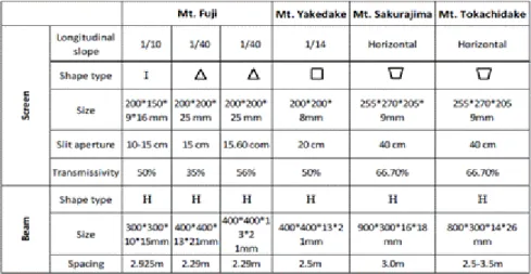
Figure 3.8 The debris flow run-out distance on the rack versus the size of openings of the rack under various material conditions (d is the median diameter size, is the density, s is the friction angle) (Gonda, 2009). ... 63 Figure 3.9 Reduction rate of run-out distance. The Cases (0-5) refer to different opening size of rack and A, B and C are the examined materials (Kim et al., 2012a). ... 64 Figure 3.10 Photos of representative flume test results (Brunkal, 2015).65 Figure 3.11 Estimated and recorded design volumes versus Catchment area in British Columbia (Lo, 2000)... 67 Figure 3.12 Peak discharge versus total debris flow (Lo, 2000). ... 68 Figure 3.13 Storage angle definition (A) and the relationship with storage basin capacity (B) (VanDine, 1996). ... 70 Figure 3.14 Components of a storage basin with an open check dam: (a) inlet structure: solid body dam; (b) scour protection; (c) basin; (d) lateral dikes; (e) maintenance access; (f) open check dam; (g) counter dam (Zollinger 1983, Piton and Pecking, 2015). ... 72 Figure 3.15 Plan and longitudinal sections of a storage basin with check dam downstream: (a) hydraulic control of the deposits: this condition is induced by an obstacle to the flow (narrower dam openings when compared to the natural channel section) (b) mechanical control of the deposits: boulders and driftwood jamming leading to open check dam clogging; (c) mixed controlled deposits: hydraulic control and mechanical control (Lange and Bezzola 2006, Piton and Pecking, 2015). ... 73 Figure 3.16 Determination of minimum spacing between dams (VanDine, 1996). ... 74 Figure 3.17 Characteristics of six racks installed in Japan (Brunkal, 2015). For the components of rack, see Figure 3.4. ... 75 Figure 4.1 Subcritical flow depths and Froude numbers near the channel exit (Campbell, 1985). ... 78 Figure 4.2 Froude numbers close to the channel exit as a function of channel geometry and material type (Campbell, 1985). ... 79 Figure 4.3 Froude numbers as a function of h/hstop a) for different channel
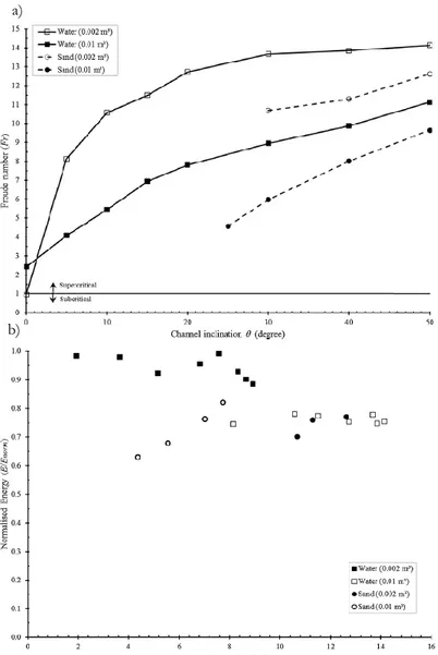
slope “” and b) for ascending rough surfaces “system 1-4” (Pouliquen, 1999). ... 80 Figure 4.4 a) Froude numbers as a function of channel slope and b) normalized energy (Choi et al., 2015). ... 82 Figure 4.5 Graphical interpretation to identify the critical height (red line) (Pudasaini et al., 2007). ... 83
11 (n). ... 84 Figure 4.7 Inclined channel used for the numerical modeling of granular material. The material enters into the channel at x = 0 with an inlet height equal to 15 cm and an average inlet velocity of 0.9 m/s (Domnik and Pudasaini 2012). ... 86 Figure 4.8 Flow depth and velocity for three different basal boundary conditions: a) no-slip; b) free-slip and c) Coulomb friction law with friction angle equal to 25° (Domnik and Pudasaini 2012). ... 87 Figure 4.9 Generalized Froude number for Coulomb friction law with friction angle equal to 25°(Domnik and Pudasaini 2012). ... 87 Figure 4.10 A possible domain decomposition: the 2D model supplies the velocities u, w, and the pressure p; the 1D model provides the flow depth h and the depth-averaged downslope velocity ū (Domnik et al., 2013). ... 88 Figure 4.11 Simulation of the velocity component in the flow depth direction (w) and shallowness parameter, in the vicinity of the silo inlet (located at x = 0) (Domnik et al., 2013). ... 89 Figure 4.12 Schematic vertical cross section of a debris flow (Iverson et al., 2010). ... 90 Figure 5.1 Channel and initial mass geometry (Rendina et al., 2017). ... 98 Figure 5.2 Lax-Friedrichs scheme (Rendina et al., 2017). ... 99 Figure 5.3 Height, velocity and Froude number of a water flow at t*=0.03 (Rendina et al., 2017). ... 101 Figure 5.4 Height, velocity and Froude number of a water flow at t*=0.05 (Rendina et al., 2017). ... 102 Figure 5.5 Froude numbers computed by FV model of a water flow on an horizontal channel with hin=1m for different dimensionless roughness index of the flow (Rendina et al., 2017). ... 103 Figure 5.6 Froude numbers of the flows computed by FV model with hin=10m for different channel slope and dimensionless dynamic viscosity
of the flow (Rendina et al., 2017). ... 104 Figure 5.7 Froude numbers of the flows computed by FV model with hin=5m for different channel slope and dimensionless dynamic viscosity
of the flow (Rendina et al., 2017). ... 105 Figure 5.8 Froude numbers of the flows computed by FV model with hin=1m for different channel slope and dimensionless dynamic viscosity
12
Figure 5.9 Trend of numerator and denominator of the Froude numbers computed by FV model for different dimensionless dynamic viscosities of the flow (Rendina et al., 2017). ... 108 Figure 5.10 Comparison of the Froude numbers computed by FV model and Flow-3D model for two different dimensionless dynamic viscosities of the flow. The legend refers to different channel slope and the colors refer to the different initial height of the flow. The hin=10m is represented in red, the hin=5m in green and hin=1m in blue (Rendina et
al., 2017). ... 109 Figure 5.11 Flow height and velocity computed by FV model in a section x’=0.05 for different dynamic viscosity of the flow and channel slope. The colors refer to the different initial height of the flow. The hin=10m is
represented in red, the hin=5m in green and hin=1m in blue (Rendina et
al., 2017). ... 112 Figure 5.12 Flow height and velocity computed by FV model in a section x’=0.10 for different dynamic viscosity of the flow and channel slope. The colors refer to the different initial height of the flow. The hin=10m is
represented in red, the hin=5m in green and hin=1m in blue (Rendina et
al., 2017). ... 113 Figure 5.13 Flow heights at a generic cross-section (x’1) for increasing dimensionless viscosities. The condition (1) corresponds to flow height with lower viscosity, while the condition (3) corresponds to flow height with higher viscosity (Rendina et al., 2017). ... 113 Figure 6.1 a) Schematic of a Digital Terrain Model (DTM), in black, over which a landslide mass is propagation, in red, (Pastor et al., 2014); b) initial and deformed configuration of a column of the landslide mass (Pastor et al., 2015a). ... 119 Figure 6.2 Numerical integration in a SPH model (Pastor et al., 2009).124 Figure 6.3 USGS flume geometry: longitudinal profile of the flume and geometry of static debris loaded behind the head-gate. The points in red indicate where the propagation heights and basal pore pressures were measured: A (x = 32 m) and B (x = 66 m) are inside the channel, while C (x = 90 m) is at the exit of the channel in a sub-horizontal open plain (Iverson et al., 2010)... 129 Figure 6.4 a) Aggregated time series data for SGM rough-bed experiments. Mean values (black lines) and standard deviations (gray shaded areas) are shown (Iverson et al., 2010); b) aggregated time series data for the flume experiment of 13 September 2001 (Iverson, 2003). 130
13 the indication of the mass at the early stages of the test before the opening of the gate. ... 134 Figure 6.6 Comparison of the flume test measurements and numerical simulations: evolution of flow depth (h) at the points A and B. ... 135 Figure 6.7 Comparison of the flume test measurements and numerical simulations: evolution of basal pore water pressure (Pwb) at the points A and B. ... 136 Figure 6.8 Comparison of the experimental measurements and the numerical simulations: a) peak of the propagation height (h); and b) peak of the basal pore water pressure (pb
w) at points A and B. The legend refers to the experimental of Figure 6.4a, b. The simulations with SPH model are represented with empty symbol, while the simulations with SPH-FDM model are represented with solid black and solid blue. The results are compared to the mean values and standard deviation (s) of the measurements at the point A (PA) and B (PB). ... 137 Figure 6.9 Computed height with SPH-FDM and FV methods of a water flow at t=0.3s and t=0.5s. ... 140 Figure 6.10 Computed velocity with SPH-FDM and FV methods of a water flow at t=0.3s and t=0.5s. ... 141 Figure 6.11 Computed Froude number with SPH-FDM and FV methods of a water flow at t=0.3s and t=0.5s. ... 142 Figure 6.12 Froude number of Frictional flow with hin=10 and 5m for
different channel slope and frictional angle of the flow. ... 144 Figure 6.13 Froude number of Frictional flow with hin=1m for different
channel slope and frictional angle of the flow. ... 145 Figure 6.14 Acceleration terms of a water flow in open channel (from Richardson and Julien, 1994). ... 146 Figure 7.1 Antelao Mountain and Cancia catchement (Borca di Cadore) located in the Northern Italian Dolomite Alps, N 46°25’30.22”, E 12°14’19.95” (Cascini, 2011). ... 151 Figure 7.2 Deposition zones of the debris flows occurred in 1868, 1994 and 1996 (Bacchini and Zannoni, 2003). ... 154 Figure 7.3 Frequency-Magnitude (F-M) curves computed for the Cancia catchment. ... 155 Figure 7.4 Some effects caused by the events dated 18th July 2009: a) buildings location; b) location of building 1 in storage basin; c), d), e) post-events traces on building 1; f), g) erosion zones and h) post-events traces on building 2. ... 158
14
Figure 7.5 DTM used for the numerical modelling of the flows occurred in 2009: a) topography pre-failure (storage basin empty) and, b) post-failure (storage basin filled) (data from LIDAR survey) and c) longitudinal and cross-sections of the DTMs pre- and post-failure. ... 163 Figure 7.6 a) DTM used for the numerical modelling of the flows occurred in 1994 and 1996 (data from LIDAR survey), b) DTM longitudinal section. ... 164 Figure 7.7 a) Plan-view extracted from DTM of Figure 7.5a of the deposition zone of the July 2009 flows, b) Longitudinal section and deposition slope. ... 165 Figure 7.8 a) Rainfall data recorded at rain gauge station of Rovina Bassa di Cancia, runoff computed at the catchment outlet b) water discharge (hydrograph) and c) cumulative volume of water. (data from Cascini, 2011). ... 168 Figure 7.9 a) Deposition thickness simulated for the 1994 events (DF and FF) with different rheological parameters; the black line represents the boundary of deposit observed in the field; b) frequency distribution of the Froude number computed within the SPH computational points (ntot = 5040) used for 1994 and 1996 events, at the time lapses when the flows reached the target run-out distances (i.e. cross-sections 1-6 of Figure 7.6). ... 172 Figure 7.10 a) Deposition thickness simulated for the 1996 event with different rheological parameters; the black line represents the boundary of deposit observed in the field; b) frequency distribution of the Froude number computed within the SPH computational points (ntot = 5040) used for 1994 and 1996, at the time lapses when the flows reached the target run-out distances (i.e. cross-sections 1-6 of Figure 7.6). ... 172 Figure 7.11 a) Final deposition thicknesses computed for the 30’000 m3 DF (scenarios 1, 2a, 2b of Table 7.2) propagating inside the Storage Basin Empty (SBE) and simulated through a frictional-type model. b) Scenario 8 of Table 7.2 propagating inside the Storage Basin Empty (SBE) and simulated through frictional-type model with internal pore water pressure. ... 175 Figure 7.12 Final deposition thicknesses computed for the 1,500 m3 FF scenarios 3-4 of Table 7.2 propagating inside the a) Storage Basin Empty (SBE) or b) Storage Basin Filled (SBF), both simulated through frictional-type model. c) Scenario 13 of Table 7.2 propagating inside the Storage Basin Filled (SBF) and simulated through Chezy-Manning model. ... 176
15 of Table 7.2) b) Longitudinal section and deposition height of FF (Case 4 of Table 7.2)... 177 Figure 7.14 Frequency distribution of the Froude number computed within the SPH computational points (ntot = 5040) used for DF and FF (2009 event), at the time lapses when the flows reached the target run-out distances (i.e. cross-sections 1-5 of Figure 7.5). ... 179 Figure 8.1 Overview of the 1998 Pizzo D’Alvano landslides and location of the selected area (modified from Cascini et al., 2011). ... 184 Figure 8.2 Geological map of Pizzo D’Alvano massif: 1) calcarenites and calcirudites (Upper Cretaceous), 2) calcarenites, calcilutites and dolomitized limestone (Middle-Upper Cretaceous), 3) marly limestone (Middle Cretaceous), 4) microcrystalline limestone partially dolomitized (Lower-MiddleCretaceous), 5) dolomized limestone (Lower Cretaceous) (Cascini et al., 2008). ... 185 Figure 8.3 Hydro-structural map of Pizzo D’Alvano massif (Cascini et al.,2008). ... 186 Figure 8.4 Overview of the “Tuostolo” mountain basin and 1998 landslides (Cascini et al. 2014). ... 187 Figure 8.5 Morphological zoning and some effects of 1998 landslides (modified from Cascini, 2006). ... 188 Figure 8.6 Overview of Pizzo D’Alvano massif just after the 1998 events (modified from Cascini, 2006). ... 189 Figure 8.7 Overview of Pizzo D’Alvano massif with control works in 2010. ... 190 Figure 8.8 Overview of control works in Tuostolo basin. ... 191 Figure 8.9 Map of pyroclastic deposits thickness: A) h=0 m, B) h<0.5 m, C) 0.5m<h<1m, D) 1m<h<2m, E) 2m<h<5m, F) h>5m) (modified from Cascini et al., 2006). ... 193 Figure 8.10 Overview of the in-situ investigations for the Tuostolo basin and stratigraphic characterization of the slope section (modified from Cascini et al., 2005). ... 194 Figure 8.11 a) Output of the SHALSTAB code with reference to the May 1998 events in Tuostolo basin: 1) ZOB areas of the sample basin, 2) observed source areas, 3) simulated source areas (modified from Cascini et al., 2005). b) Output of the TRIGRS code (Sica, 2008). ... 195 Figure 8.12 The landslide source areas and the final deposition thicknesses computed for the Tuostolo basin (modified from Cascini et al., 2014). ... 196
16
Figure 8.13 DTMs and source areas used for the numerical modelling of the flows. ... 199 Figure 8.14 Longitudinal sections of the DTMs. ... 200 Figure 8.15 Several combination of two DTMs (DTM and DTM CW) used for the numerical modelling of the flows. ... 202 Figure 8.16 Check dams, channel and storage basin filled by vegetation (photo taken in September 2017). ... 202 Figure 8.17 The obtained triggering masses. The location of source areas is shown in Figure 8.13. ... 203 Figure 8.18 a) Deposition thickness simulated by Cascini et al., 2014 for the 1998 event; b)simulated deposition thickness using the 11 DTM of Figure 8.13a and c) the 11 DTM of Figure 8.15a. The black line represents the boundary of deposit observed in the field. ... 205 Figure 8.19 Froude number along section “s” computed at the time lapses when the flows reached the cross-sections 1-5. ... 206 Figure 8.20 Final deposition thicknesses computed for the 75’000 m3 event: scenarios 1, 2, 3 and 4 of Table 8.1. ... 208 Figure 8.21 Final deposition thicknesses computed for the 145’000 m3 event: secenarios 4b and 5b of Table 8.1. ... 209 Figure 8.22 Froude number along section “s” computed at the time lapses when the flows of Figure 8.20 reached the cross-sections 1-5. .. 210 Figure 9.1 Structure of a debris-flow dewatering brake. ... 215 Figure 9.2 Experimental channel: longitudinal profile of the channel (wide 20 cm) and geometry of the initial mass. At the downstream end of the channel there is a (permeable) rack (Gonda, 2009). ... 215 Figure 9.3 The variation of the debris flow run-out measured by Gonda (2009), using the material “A” and different sizes of the openings of the rack (from Cascini et al., 2016a,b). ... 217 Figure 9.4 Vertical profiles of the computed relative pore water pressure (pwrel) without (a) and with (b) a draining boundary condition (i.e. p
wrel assigned equal to zero) in the horizontal terminal part of the channel where the rack is located (from Cascini et al., 2016a,b). ... 220 Figure 9.5 Comparison of the experimental measurements and the numerical simulations of the run-out distances on the rack for the tests of Table 9.1. The legend refers to the different material and channel slope and the numbers represent the experimental conditions of the Table 9.1 (from Cascini et al., 2016a,b). ... 221
17 within the SPH computational points (ntot = 1000) used for numerical modeling of Case 1 (a) and Case 2 (b), at the significant times. ... 223 Figure 9.7 Final deposition thicknesses computed for a saturated volume of 75’000 m3 without rack (a) and with rack in the first storage basin (b). ... 225 Figure 9.8 Froude number along section “s” a) without rack and b) with rack computed at the time lapses when the flows reached the cross-sections 1-5. ... 226
19 Table 2.1 Most common rheological models used to describe landslides behavior (modified from Quan Luna, 2012). ... 45 Table 2.2 Most common numerical models (Quan Luna, 2012)... 46 Table 2.3 The proposed rheological models for each type of flow like mass-movements. ... 49 Table 3.1 Design input data for passive control works. ... 71 Table 5.1 List of analyzed cases for viscoplastic flows with hin=10 m; in
bold the corresponding Froude numbers computed by FV model (Rendina et al., 2017). ... 106 Table 5.2 List of analyzed cases for viscoplastic flows with hin=5 m; in
bold the corresponding Froude numbers computed by FV model (Rendina et al., 2017). ... 107 Table 5.3 List of analyzed cases for viscoplastic flows with hin=1 m; in
bold the corresponding Froude numbers computed by FV model (Rendina et al., 2017). ... 107 Table 5.4 Percent Variation (PV) of flow height (PV(h)), velocity (PV(u) and Froude number (PV(Fr)) in the sections x’=0.05 and x’=0.10 (Rendina et al., 2017). ... 114 Table 6.1 Geotechnical properties of soils for the SGM rough bed experiment (Iverson et al., 2010). ... 128 Table 6.2 Rheological parameters for the numerical simulations of the flume tests performed by (Iverson et al., 2010). ... 138 Table 7.1 Past events at the Borca di Cadore cacthment. ... 153 Table 7.2 List of numerical cases analysed for the back-analysis of the 2009 events. ... 173 Table 8.1 List of numerical cases analysed for future events. ... 207 Table 9.1 Flume tests of Gonda (2009) selected for the numerical modelling. ... 217 Table 9.2 Rheological parameters for the numerical simulations of the flume tests performed by Gonda (2009). ... 219
21 Flow-like mass movements are catastrophic events occurring all over the world and may result in a great number of casualties and widespread damages. The analysis of the time-space evolution of the kinematic quantities is a useful tool to understand the propagation stage of these phenomena as well as for control works design.
The thesis deals with study of flow regime of Newtonian and non-Newtonian fluids and provides a contribution to this topic through the use of numerical procedures based on FV (finite volume) scheme and SPH (smoothed particle hydrodynamics) method. The FV model, developed by Rendina et al., 2017, is a single phase equivalent model, while the Geoflow-SPH, developed by Pastor et al.2009, considers the propagating mass with an average behavior of solid skeleton and pore water pressure.
The flow kinematics are analyzed through the Froude number, widely used in hydraulic engineering, discriminates two different kinematical features i.e. subcritical (slow) or supercritical (rapid) flows. The analysis concern a 1D/2D dam break of Newtonian (water flow) and non-Newtonian flows (in particular based on a viscoplastic and frictional laws).
The numerical results highlighted flows are supercritical even in areas far from trigger zones and Froude numbers of viscoplastic flows are higher than frictional flows.
Later, the Froude number is used as a quantitative descriptor of the control works response and, more generally, as an useful tool to estimate the efficiency of existing storage basins. The first case study regards Cancia, in the Dolomite Alps, where two storage basins dramatically failed on 2009 due to a short-time sequence of rainfall-induced debris flows and flash floods. The kinematic analysis highlighted that debris flow can be associated to a subcritical flow while flash flood is similar to a supercritical flow and for latter lower is the potential efficacy of control works.
The second case study regards Sarno, in the Campania region, where one of the most complex systems of passive control works was built after the 1998 events. The performance of the protection system is analyzed
22
referring to Froude number again which highlighted the importance of planning the emergency/ordinary maintenance of control works.
Finally, a new type of passive control work is described, i.e. the permeable rack that has the function of decrease the pore water pressures at the base and inside the propagating mass, thus causing the landslide body to brake and stop. The rack performance is tested as adaptation structure in existing protection systems also.
23
ACKNOWLEDGENTS
I would like to express my sincere gratitude to my supervisors, Leonardo Cascini, Sabatino Cuomo, Giacomo Viccione and Manuel Pastor for the guidance, encouragement and advice they have provided throughout my PhD studies and related research. It was a real privilege and an honour for me to share of their exceptional scientific knowledge but also of their extraordinary human qualities. I would like to thank you for allowing me to achieve this work.
Thanks to each member of Geotechnical Engineering Laboratory of Technical University of Madrid and a special thanks to Angel for our great friendship.
Thanks to each member of Geotechnical Engineering Laboratory of University of Salerno; I have been happy to share delights and worries with a friendly and cheerful group composed by Maria Rosaria, Maria Grazia, Mariagiovanna, Antonella, Antonio, Gaetano, Pooyan, Gianfranco and Luca.
A heartfelt thanks to Vittoria, I am extremely lucky to have a friend like her.
I must express my very profound gratitude to my parents for providing me with unfailing support and continuous encouragement throughout my years of study and throughout the process of researching and writing this thesis.
Last but not the least, I want to express my special thanks to Filippo, my better half, this accomplishment would not have been possible without you. Thank you.
25 Ilaria Rendina graduates in Environmental Engineering at the University of Salerno with 110/110 cum laude. During the PhD course she developed research topics about the propagation modeling of the flow-like mass movements with reference to the interaction of the flows with passive control works. She developed a 1D and single phase numerical model with the cooperation of a Hydraulic professor of University of Salerno (UniSa). She deepened the Geoflow-SPH model at the Technical University of Madrid (UPM). She attended several research meetings and workshops about flow-like phenomena, among which the international LARAM School on landslide risk assessment and mitigation (September 2016). In 2017 she presented part of current scientific research works at the Annual Meeting of Italian Geotechnical Researchers. She is co-author of scientific papers published in international journals, international and national conference.
Ilaria Rendina si laurea in Ingegneria per l’Ambiente ed il Territorio presso l’Università di Salerno con voto 110/110 e lode. Durante il corso di Dottorato si dedica a tematiche di ricerca connesse alla modellazione della fase di propagazione di frane tipo flusso con riferimento all’interazione di tali flussi con interventi di tipo passivo. Ha sviluppato un modello numerico monodimensionale e monofase in collaborazione con un professore di Idraulica dell’Università di Salerno (UniSa). Ha approfondito in modello Geoflow-SPH presso il Politecnico di Madrid (UPM). Partecipa a diversi incontri di ricerca e workshops riguardanti fenomeni franosi tipo flusso, tra cui la scuola internazionale LARAM sulla valutazione e la mitigazione del rischio da frana (Settembre 2016). Nel 2017 ha presentato lavori scientifici all’Incontro Annuale dei Ricercatori di Geotecnica. E’ co-autrice di articoli scientifici pubblicati su riviste internazionali e in atti di convegno internazionali.
27
1 INTRODUCTION
Flow-like mass movements cause numerous victims and huge amounts of economic damage around the world. The typical features of these flow-like landslides are strictly related to the mechanical and rheological properties of the involved materials. Depending on solid fraction in the water-solid flowing mixture it is possible distinguish “debris flow” with high solid fraction (47-77%), “hyperconcentrated flow”(20-47%) and “flash flood” (<20%).
These flows are usually characterized by different magnitude (e.g. volume), runout distance (up to tens of kilometres) and velocity (in the order of metres/second).
The prediction of both runout distances and velocity through numerical modelling of the propagation stage can notably reduce losses inferred by these phenomena, as it provides a means for working out the information for the identification and design of appropriate mitigation measures (Pastor et al., 2009).
The PhD thesis focuses on understanding the flows kinematic features during the propagation phase and evaluating the effectiveness of passive control works such as check dams, storage basins and “permeable” racks. This work provides a contribution on this topic through the Froude number (Fr) expressing the ratio of inertial and gravitational forces. The Fr discriminates two different kinematical features of flow i.e. subcritical or slow (Fr <1) and supercritical or rapid flow (Fr>1) and becomes a quantitative descriptor of the control works efficiency.
Particularly, Chapter 2 proposes a literature review with reference to the main classifications of flow-like mass movements, the main stages and approaches available for propagation modeling. Finally, the main rheological models associated with each type of flow like phenomena are introduced to describe the behavior of involved material during the propagation stage.
28
Chapter 3 concerns the description of different types of passive control works, the main characteristics and design criteria, paying specific attention to “permeable” racks.
Chapter 4 summarizes the literature about Froude number focusing on experimental, analytical and numerical models analyzing the regime of flow-like mass movements.
Chapter 5 describes a 1D single phase equivalent model proposed by Rendina et al., 2017, to estimate the regime of Newtonian and non-Newtonian fluids flowing in an open channel. In particular, the kinematic of viscoplastic fluids, such as hyperconcentrated flows or flash flood, is studied.
In Chapter 6 the SPH-FDM model (proposed by Pastor et al., 2015) is used to simulate well-documented flume tests performed in USA. The validated model is later used to estimate the regime of the non-Newtonian flows in an open channel. In particular, the kinematic of frictional flows, such as debris flows or granular flows, is studied.
Chapter 7 deals with the case study of Cancia (North Italy) where some storage basins dramatically failed on 2009 due to a short-time sequence of rainfall-induced debris flows and flash floods. This issue is tackled using SPH model and implementing the Froude number to estimate the kinematical characteristics of different flows and the efficiency of control works.
Chapter 8 deals with a second case study in Sarno town (South Italy) where, after the catastrophic events of ’98, some passive control works were built. Considering that no event occurred after the control works construction, the magnitude of future events was estimated on the basis of the available data. The numerical analysis are performed through SPH model implementing the Froude number to analyze the kinematic characteristics of the flows that interact with the control works.
In Chapter 9 the SPH-FDM model is used to simulate well-documented flume tests performed in Japan, equipped with a basal rack located at the end of the channel.
29 Once tested the reliability of the SPH-FDM model to describe the behavior of a debris flow on a permeable bottom boundary, the same model was used to simulate the potential upgrading of existing passive control works in the mountain basin described in Chapter 8 through the “permeable” rack.
Finally, Chapter 10 provides a general discussion and concluding remarks based on the results obtained for each section.
31
2 FLOW-LIKE MASS MOVEMENTS
Landslides are widespread catastrophic events around the world posing high risk to life and properties. Among natural disasters causing human life losses in the world, the floods and landslides are ranked as fourth and sixth place respectively, after earthquake, tsunami and extreme temperature (Fig. 2.1). Regarding to estimated economic losses caused by landslides and floods, a total of US $ 21.3 billion damages were reported in 29 countries out of 82 onc having experienced such disasters in 2015 (EM-DAT, 2016).
The events number, victims and economic damages are different in each continent, as testified by the global statistics on major events that have occurred in 2015 (Fig. 2.2). In terms of events number, Asia had the greatest percentage (45.1%), followed by the America, Africa, Europe and Oceania. The maximum number of deaths was recorded in Asia (86.9%), whereas this percentage was very low in the case of four other continents. Finally, in 2015 the reported damages were mainly widespread in three continents: Asia, America and Europe.
32
Figure 2.1 Human life losses for different type of disaster (2015 versus average 2005-2014) (source EM-DAT www.emdat.be).
33
Figure 2.2 Percentage of reported events, victims and economic damages in
different continents for landslides and floods events in 2015 (source EM-DAT www.emdat.be).
Of particular interest are flow-like mass movements systematically producing huge amounts of damage and numerous victims because of their high velocities and large run-out distances. Such phenomena involve different type of soil and, among these, pyroclastic soils originated in Campania region (Southern Italy) from the explosive phases
34
of the Somma Vesuvius volcano (Cascini et al., 2003) or granular materials in the Italian Dolomite Alps (Northern Italy).
In the following, the main features of flow-like mass movements are analyzed with referencing to to: i) classifications proposed by literature, ii) different stages, iii) rheological characteristics and approaches for proper modeling.
2.1 C
LASSIFICATIONThe flow type mass-movements are composed of mixtures of air, steam, water and solid fractions of various nature: such as fractured rocks, sands, silts including loess and volcanic ashes, sensitive and stiff fissured clays and organic soils (Hungr et al., 2001).
In order to frame the fundamental characteristics of flow-like movements, in the following the main scientific classifications are described.
The Varnes (1978) classification distinguishes different types of landslides on the basis of the movement typology and involved material (Fig. 2.3). As regards the involved material, Varnes (1978) separates rock and soil; the latter is divided into earth and debris: earth describes material in which 80% or more of the particles are smaller than 2 mm; debris contains a significant proportion of coarse material that is from 20% to 80 % of the particles are larger than 2 mm and the remainder are less than 2 mm. With reference to the typology of movement, the author distinguishes between falls, topples, slides, spread and flows. In particular for the flows the instability does not occur as a movement on one or more sliding surfaces, but rather as a viscous fluid in which the involved material are not able to resist the tangential stress variation produced by distortional deformations.
35
Figure 2.3 Slope movement type and processes (Varnes, 1978).
The Cruden and Varnes (1996) classification considers the velocity reached by the landslide during the propagation stage (Fig. 2.4). The flow-like mass movements are included in the classes 5, 6 and 7 in Figure 2.4.
36
Figure 2.4 Landslide velocity scale (Cruden and Varnes, 1996).
The Hutchinson (1988) classification focuses on flow-like phenomena identifying: mudslides (non periglacial), periglacial mudslides (gelifluction of clays), flowslides, debris flows and sturzstroms. These phenomena differ in terms of mechanisms: In the mudslides phenomena, the shear failure process prevails over flow process; in flow slides and debris flow phenomena the two processes coexist whereas in sturzstroms just the flow processes exclusively occur (Fig. 2.5). Furthermore, among flow-like phenomena, Hutchinson (1988) distinguishes the mass transport
37 phenomena and mass movement phenomena. This distinction is based on the water content value, the unit weight of the mixture and sediment concentration (Fig. 2.6). In 2003, Hutchinson proposed a review of flow-like mass movements and identified two main groups: flow-type landslides in granular materials (debris flows, flow slide and rock avalanche) and flow-type landslides in fine-grained material or cohesive material (mudslides).
38
Figure 2.6 Continuous spectrum of sediment concentration. (Hutchinson, 1988).
Costa (1988) classification distinguishes three types of flow: Water Flood (WF), Hyperconcentrated Flow (HF) and Debris Flow (DF) as function of sediment concentration, bulk density, shear strength and flow type (Fig. 2.7).
Figure 2.7 General Rheologic Classification of Water and Sediment Flows in Channels (Costa, 1988).
39 Coussot and Meunier (1996) propose a classification of flow-like phenomena as a function of solid fraction and material type (Fig. 2.8). Furthermore the authors distinguish the one-phase flow or two-phase flow, respectively if the relative velocity of water and solid is small so that it can be considered as a viscous fluid or if the mean velocity of the coarsest solid particles, which are on the bed (bed-load), significantly differ from that of the water-solid suspension which flows around it.
Figure 2.8 Classification of flow-like phenomena as a function of solid fraction and material type (Coussot and Meunier, 1996).
Hungr et al. (2001 and 2012) proposed a complete classification on the basis of: material type; water content; presence of excess pore-pressure or liquefaction potential at the source of the landslide, presence of a defined recurrent path (channel) and deposition area (fan); velocity and peak discharge of the event (Fig. 2.9).
40
41
2.2
STAGESIn flow-like phenomena it is possible to recognize three main stages: the triggering, the propagation and the deposition stages (Hungr et al., 2001). Flow-like mass movements induced by rainfall have different features whether originated by infiltration or runoff along slopes. The first process occurs in the flows where the water prevails in the water-solid flowing mixture that, depending on solid percentage, affects “hyperconcentrated flows” (HF) (Coussout and Meunier 1996), “water floods” (WF) (Costa, 1988) and also “flash floods” (FF) (Gaume et al., 2009). This triggering mechanism involves different stages: detachment of soil particles, transportation of sediment due to soil erosion induced by intense rainfall and deposition when the transport capacity of the flow is reduced below that required for the existing suspended load (Kavvas and Govindaraju, 1992).
The “debris flows” (DF) are originated from a variety of triggering mechanisms and they are mainly related to the reduction of soil shear strength caused by the increase in the pore water pressure as a result of several factors like (Cascini et al., 2005): surface runoff processes (Van Dine, 1985; Takahashi, 1991, van Ash et al., 2009; Berti et al., 1999); increase of the water table (Leroueil, 2004; Dietrich and Montgomery, 1998); groundwater supplies provided by artesian conditions or hidden springs (Mathewson et al., 1990; Onda et al., 2004; Lacerda, 2004); groundwater flow patterns caused by the stratigraphic setting and/or anthropogenic structures and roads (Wolle and Hachich, 1989; Ng and Shi, 1998; Crosta et al., 2003); increase of saturation degree in unsaturated soils (Futai et al., 2004); variations of hydraulic boundary conditions due to the formation of deep rills as a result of erosion processes related to intense rainfall (Deere and Patton, 1972); undrained loading as a result of first time slides triggered by rainfall, that impact on in-place soils (Hutchinson and Bhandari,1971) and soil liquefaction phenomena (Sassa, 1985; Hungr et al., 2001).
The propagation stage includes the movement of the unstable masses from the source area toward the deposition. During this phase it is possible to observe erosion processes in HF, WF and FF; while fluidization phenomena along the path in DF. The erosion can be extremely important since the result of this process is an increase of the
42
landslide volume (Costa and Williams, 1984; Jibson, 1989; Sassa et al., 1997; Wieczorek et al., 2000; Cascini, 2004). On the other hand, the fluidization can occur along the sliding surface or within the sliding zone during the rise in pore-water pressure and affects both the run-out distances and the kinematic characteristics of the propagating masses (Iverson and LaHusen, 1989; Iverson and Denlinger, 2001; Iverson et al., 2010; Iverson et al., 2011; Cascini et al., 2016).
The four types of flows (DF, HF, WF, FF) are usually characterized by different magnitude (e.g. volume), runout distance and maximum velocity at piedmont areas where urban centres are usually settled. The high discharge of debris flows, up to 40 times greater than those of extreme floods, (Hungr et al., 2001) is responsible for greater flow depth (up to 20 m), higher velocity (up to 30 m/s) and higher impact loads respect to hyperconcentrated flows.
When the flows reach the apex of the depositional fan, it is possible to recognize different deposit structures: in the HF, WF and FF the coarsest solid fraction generally deposits first whereas the fine suspension flows away as wash load before being deposited during flow; in the DF the concentration of big boulders is higher close to the surge front (Coussot and Meunier, 1996).
2.3 A
PPROACHES FOR MODELINGThe features of flow-like mass movements provide serious difficulties towards their complete modelling and several models are used to interpret separately the different stages.
Focusing on the propagation stage, it is usually deepened through empirical and analytical methods, small or large-scale laboratory tests and finally through numerical methods.
43 Empirical methods (e.g. Corominas, 1996) are usually based on extensive amounts of field observations and on the analysis of the relationships between the run-out distance and different landslide mechanisms, their morphometric parameters, the volume of the landslide mass and the physical and mechanicals characteristics of soils (Quan Luna, 2012). These methods are based on very simplified conditions and it is possible to use them only for conditions similar to those on which their development is based.
Analytical methods (e.g. Takahashi, 1991) include different formulations based on lumped mass approaches in which the mass is assumed as a single point (Quan Luna, 2012). These methods have an obvious limitations in being unable to account for internal deformation and the motion of the flow front; but they may provide reasonable approximations to the movement of the center of gravity of the landslide (Evans et al., 1994).
Small or large scale laboratory tests (e.g. Iverson et al., 2010) are used to measure the kinematic characteristics of the flows in order to understand the flow- like mass movements behavior. These tests provide a dataset in order to test the numerical models used to interpret and predict landslides.
Numerical methods (e.g. Pastor et al., 2009) have been developed either for distinct element or for continuum based models. Continuum fluid mechanics models, the most common approach, are based on the mass, momentum and energy conservation equations that describe the dynamic motion of flow and a rheological model to describe the landslide behavior (Quan Luna, 2012).
The numerical methods can be classified in three groups: model based on the solution dimension in 1D or 2D; models based on the solution reference frame and models based on the basal rheology.
44
Models based on the solution dimension in 1D or 2D: 1D models analyze the movement considering the topography as a cross-section of a single predefined width while 2D models make the analysis considering the topography in plan and cross-section (De Chiara, 2014);
Models based on the solution reference frame: the equation of motion can be formulated in two difference frames of reference: Eulerian or Lagrangian. An Eulerian reference frame is fixed in space, analogous to an observer standing still as a landslide passes, and require the solution of a governing equation using a dense, fixed computational grid. A Lagrangian reference frame moves with the local velocity, analogous to an observer riding on top of landslide (De Chiara, 2014);
Models based on the basal rheology: the rheology is defined as the study of the flow behavior (Irgens, 2014) and is expressed as resistance forces (τb) that interacts at the interface between the flow and the bed path (Quan Luna, 2012). The most common rheological models used to describe landslides behavior are: “Newtonian resistance”, “frictional or Coulomb resistance”, “frictional-turbulent or Voellmy resistance”, “visco-plastic or Bingham or Herschel-Bulkey resistance” and “Quadratic resistance” (Luna, 2012) (Table 2.1). The flow resistance term may be broadly separated into: one-phase models which describe the flow resistance behavior of either the slurry of water and fine material or the entire fluid-solid mixture and two-phase models which consider both a fluid phase and a solid phase (Naef et al., 2006). An overview of several numerical models as a function of rheology, solution approach and reference frame is represented in Table 2.2.
45
Table 2.1 Most common rheological models used to describe landslides behavior (modified from Quan Luna, 2012).
Reology Description Flow resistance term (τb)
Chezy-Manning (Newtonian -turbulent) Resistance that is a function of flow depth, velocity and turbulent coefficient (Manning coefficient) (m) (Pastor et al., 2009).
(2.1) With: ρ the flow density; g the gravitational acceleration; m’ the Manning coefficient that takes into account the turbulent and dispersive components of flow; u the flow velocity and h the flow height.
Frictional
(Coulomb) Resistance based on the relation of the effective bed and normal stress at the base and the pore fluide pressure (Pastor et al., 2009)
and
and
(2.2)
With: b the basal friction angle; the dynamic frictional angle and ru the
pore-pressure ratio.
Voellmy Resistance that
features a velocity squared resistance term (turbulent coefficient ξ) similar to the square value of the Chezy resistance for turbulent water flow in open channels and a Coulomb-like friction (apparent friction coefficient ε). (Voellmy, 1955).
(2.3) With: ε equal to Frictional resistance (2.2); u the flow velocity; ξ is the turbulent coefficient and h the flow height.
Bingham Resistance that is a
function of flow depth, velocity, constant yield strength (τy) and dynamic
viscosity (μ) (Coussot, 1997).
(2.4)
With: ρ the flow density; g the gravitational acceleration; h flow height; τy the constant yield
strength due to cohesion; μ dynamic viscosity and u flow velocity.
46
Quadratic Resistance that
incorporates a turbulent contribution to the yield and the viscous term already defined in the Bingham equation (O’Brien et al., 1993).
(2.5) With: τy the constant yield strength due to
cohesion; ρ the flow density; g the gravitational acceleration; h flow height; K the resistance parameter that equals for laminar flow in smooth, wide, rectangular channels, but increases with roughness and irregular cross sections; μ dynamic viscosity; u flow velocity and m’ Manning coefficient.
Table 2.2 Most common numerical models (Quan Luna, 2012).
Model Rheology Solution
approach Reference frame Variation of rheology MADFLOW
(Chen and Lee, 2007)
Frictional, Voellmy and
Bingham
Continuum
Integrated Lagrangian with mesh No
TOCHNOG
(Crosta et al., 2003) (elastoplastic Frictional model)
Continuum
Integrated Differential (adaptive mesh) Yes RAMMS (Christen et al., 2010) Voellmy Continuum
Integrated Eulerian Yes
DAN3D (Hungr and McDougall, 2009) Frictional, Voellmy and Bingham Continuum
Integrated Lagrangian Yes
FLATMODEL
(Medina et al., 2008)
Frictional and
Voellmy Continuum Integrated Eulerian No
SCIDDICA S3-hex
(D'Ambrosio et al., 2003)
Energy based Cellular
Automata Eulerian No
3dDMM
(Kwan and Sun, 2006)
Frictional and
Voellmy Continuum Integrated Eulerian Yes
SPH
47 Bingham MassMov2D (Begueria et al., 2009) Voellmy and
Bingham Continuum Integrated Eulerian Yes
RASH 3D (Pirulli and Mangeney, 2008) Frictional, Voellmy, Quadratic Continuum Integrated Eulerian No FLO-2D
(O' Brien et al., 1993)
Quadratic Continuum
Integrated Eulerian No
TITAN2D
(Pitman and Le, 2005)
Frictional Continuum
Integrated Lagrangian with mesh No
PFC
(Poisel and Preh, 2007)
Inter-particle and particle wall
interaction Solution of motion of particles Distinct element method No VolcFlow (Kelfoun and Druitt, 2005) Frictional and
Voellmy Continuum Integrated Eulerian No
2.4 D
ISCUSSIONThe proposed classifications in the literature introduce a framework for i) type of movement and type of material; ii) velocity class; iii) solid fraction and water content and iv) genesis mechanisms and evolution. However, different limits can be recognized in the classifications, mainly due to: i) different terminology used to identify the phenomenon; ii) difficulty to make distinction between different phenomena iii) not exhaustive description of triggering and evolution mechanisms.
An open issue for propagation modeling is the selection of suitable rheological model for each type of flow-like mass movements. The difficulties arise from variability of landslides composition (solid fraction and water content) that changes within the wave and along the flow
48
path. Another major difficulty is distinguishing between appropriate flow regimes, which may also change during the propagation phase. In order to choose the most appropriate rheological model it is important to understand if the fine or coarser particles dominate the flow behavior. According to Coussot and Meunier Classification, the “mudflows” (MF) and “landslides or earthflows” (EF) belong to the first group; while “debris flows” (DF) and “granular flows” (GF) to the second group. For both groups, during the propagation stage, solid particles and water move at the same velocity as a single visco-plastic body (one-phase flow) in a laminar flow, undergoing large homogeneous deformations without significant changes to its mechanical properties (Coussot and Meunier, 1996). Therefore, these flows exhibit a behavior well described by a visco-plastic rheological models such as the Bingham model or the Herschel-Bulkley model (Eq. 2.4).
Actually, in the case of high velocities of the flow, the DF and GF may show turbulent behavior, suggesting that laminar flow resistance relations may be inappropriate; indeed for these flows the grain collisions dominate the flow behavior. So, they may be described by Newtonian resistance (Eq. 2.1), frictional or Coulomb resistance (Eq.2.2) and frictional-turbulent or Voellmy resistance (Eq. 2.3).
The HF may be generalized as a turbulent, solid–liquid two-phase flow, gravity-driven flows of water and sediment in which the mean velocity of the coarsest solid particles, which are pushed and rolled on the bed (bed-load), significantly differ from that of the water-solid suspension which flows around it (Coussot and Meunier, 1996).
The WF and FF with low concentration of sediment, high percentages of fine material and low strain rates follow a Newtonian behaviour (Costa, 1988); since the increament of the sediment concentrations (HF) the flow mechanism begins to change: viscosity and shear strength as well as increasing particle collisions so that the flows exhibit a behaviour could be well described by a viscous-plastic rheological models such as
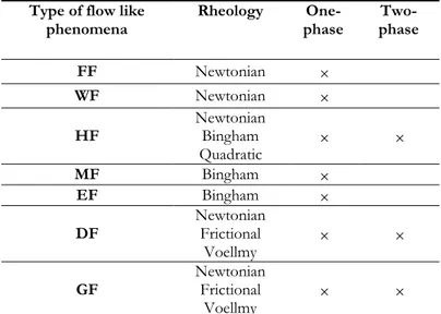
49 the Bingham model (Eq. 2.4) or a collisional-viscous-plastic rheological model like the quadratic shear stress model (Eq. 2.5). In the Table 2.3 or Figure 2.10 the main rheologies associated with each type of flow like phenomena are shown; the proposed rheological models are used in all modeling of the flow-like mass movements analyzed in this PhD thesis.
Table 2.3 The proposed rheological models for each type of flow like mass-movements.
Type of flow like
phenomena Rheology phase One- phase
Two-FF Newtonian WF Newtonian HF Newtonian Bingham Quadratic MF Bingham EF Bingham DF Newtonian Frictional Voellmy GF Newtonian Frictional Voellmy
MF: mudflows; EF: earthflows; FF: flash floods; WF: water flows; HF: hyper-concentrated flows; DF: debris flows and GF: granular flows.
50
DA
Frictional
WATER SOLID
Increasing solid fraction
Increasing water content
Stability GF Newtonian Frictional Voellmy EF Bingham Rapid motion DF Newtonian Frictional Voellmy FF -WF Newtonian HF Newtonian Bingham Quadratic Rockfalls MF Bingham
Figure 2.10 The proposed rheological models for each type of flow like mass-movements. MF: mudflows; EF: earthflows; FF: flash floods; WF: water flows; HF: hyper-concentrated flows; DF: debris flows; GF: granular flows and DA: debris avalanches.
51
3 PASSIVE CONTROL WORKS
Flow-like mass movements consequence can be reduced through landslide risk mitigation measures, which include non-structural and structural measures. Non-structural measures are based on early-warning and alarm systems or civil protection plans, both able to increase the awareness and the preparedness of the persons at risk. Structural measures include drainage, erosion protection, channelling, vegetation, ground improvement, barriers such as earth ramparts, walls, artificial elevated land, anchoring systems and retaining structures; buildings designed and/or placed in locations to withstand the impact forces of landslides and to provide safe dwellings for people, and escape routes (Vaciago, 2013). All these measures, Figure 3.1, can be broadly divided into two groups: active and passive control works. Their function is to avoid the landslide triggering or to stop/diverge the flows or to diminish their impact to the exposed structures.
52
53 The selection of the most appropriate mitigation measures depends on several aspects: the physical characteristics of the geosystem, including the stratigraphy and the mechanical characteristics of the materials, the hydrological (surface water) and the hydrogeological (groundwater) regime; the morphology of the area; the actual or potential causative processes affecting the geosystem, which can determine the occurrence of movement or landslides; the presence and vulnerability of elements at risk, either in the potentially unstable area or in areas which may be affected by the run-out; the phase and rate of movement at the time of implementation; the morphology of the area in relation to accessibility and safety of workers and the public; environmental constraints, such as the impact on the archeological, hystorical and visual/landscape value of the locale; preexisting structures and infrastructure that may be affected, directly or indirectly and capital and operating cost, including maintenance (Vaciago, 2003).
In the following the attention is focused on typologies and design criteria of passive control works.
3.1 T
YPE OF PASSIVE CONTROL WORKSThese control works can be divided into three basic types: open, closed and sediment control structures.
Open control works are designed to “constrain” the flow while closed control works are designed to “contain” the flow; finally, the sediment control structures to control the movement of fine-grained material across a debris fan or alluvial fan, thereby minimizing the amount of fine-grained sediment entering a neighbouring body of water (VanDine, 1996).
The open control works include: i) unconfined deposition areas, ii) impediments to flow (baffles), iii) check dams, iv) lateral walls (berms), v) deflection walls (berms) and vi) terminal walls, berms, or barriers.
54
The unconfined deposition area (Fig. 3.2 a) are designed to slow down and prepare the flow to the deposition phase through low slopes and extended cross-sections. This type of control works can be associated with impediment to flow or baffles to deflect the flow (Fig. 3.2 b). The check dams are usually built in series in the transportation/amplification zone of a flow like phenomenon or immediately upstream of a storage basin. In the first case are used to reduce the channel slope locally and the erosion process along the bottom and sides of the channel (Fig. 3.2 c); in the latter case, the dams are intended to be inlet control structures. The lateral walls and deflection walls are designed to constrain the lateral movement of flow and to protect buildings along the path of flow like phenomena (Fig. 3.2 d); while the terminal wall to encourage deposition by presenting obstruction to flow (Fig. 3.2 e).
55
Figure 3.2 An overview of open control works: a) unconfined deposition areas; b) baffles; c) check dams; d) lateral walls; e) deflection walls and f) terminal wall (VanDine, 1996).
56
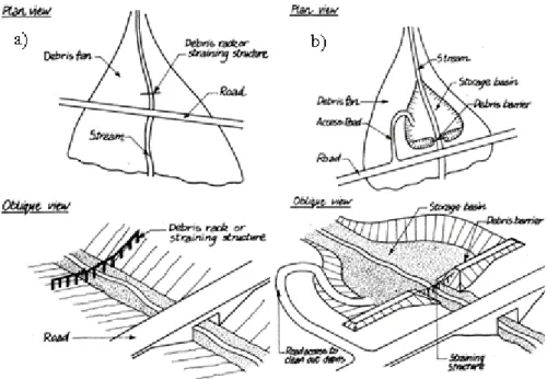
The closed control works include: debris racks, grizzlies, or some other form of debris-straining structure located in the channel; and debris barriers (or open dams) and storage basins (VanDine, 1996).
The debris racks and debris barriers are used to separate fine and coarser particles from water flows, (Figs. 3.3 a, b), while the storage basins are similar to terminal berm or barrier, in that both are located across the debris flow path and designed to encourage deposition (Fig. 3.3 b).
Figure 3.3 An overview of closed control works: a) debris racks and debris barriers (or open dams) and storage basins (VanDine, 1996).
The sediment control structures are designed to remove water from debris flow and thus to reduce flow energy. In the following, a particular sediment control work is described in detail considering that its use is analyzed in the following as a relevant measure to upgrade existing control works.
57 3.1.1 The permeable rack
The permeable rack or debris-flow brake is an old-new sediment control structure based on the dissipation of pore water pressures during the propagation of a debris flow. This control work can be located along the path of the landslide and is a unique sediment-control facility designed to reduce the run-out distance of debris flows. It consists of a “screen” which is a flat drain-like deck placed horizontally over the river channel (Fig. 3.4); when a debris flow crosses the drainage, the velocity of the debris flow decreases rapidly and then it stops (Cascini et al., 2016). The basic idea of this control work was proposed by Hashimoto and other Japanese scholars in the fifties (Kiyono et al., 1986). Debris-flow brakes were tested in three pilot projects in Japan to collect data and technical know-how regarding their construction and maintenance; then, a real-size experiment carried out in the Kamikamihori Valley, Mt. Yakedake, Nagano Prefecture, Japan (Gonda, 2009; ICHARM,2008). A permeable rack was installed in 1985 on a 4° slope parallel to the original stream channel slope. The board consisted of 25 prismatic steel pipes, each 20 m long with rectangular cross-sections of 0.2 × 0.2 m. The pipes were laid parallel to each other with 0.2-m spaces between them to drain off the watery slurry when subjected to debris flows (Fig. 3.5) (Suwa et al., 2009).
58
59
Figure 3.5 Structure of the rack in Kamikamihori Valley, Mt. Yakedake, Nagano Prefecture, Japana (Kiyono et al., 1986).
Six days after the completion of the rack construction ( July 21, 1985), a debris flow event occurred. The Figure 3.6 shows the characteristics of the event while the Figure 3.7 shows two screenshots before and after
60
the occurrence of the event. Only 5% of the total volume of 5500 m3 stopped, however the peak of the flow rate must have been effectively reduced and the flow converted to a less-harmful level because of the reduced size of the front grain (Suwa et al., 2009).
Figure 3.6 Hydrograph of the July 21, 1985 debris flow showing the gravel content and size parameters (Suwa et al., 2009).
61
Figure 3.7 Pictures of a permeable rack, before and after the occurrence of a debris flow in the Kamikamihori Valley, Mt. Yakedake, Nagano Prefecture, Japan (Cascini et al., 2016).
Since few years the efficacy and the efficiency of permeable racks have been experimentally tested by Gonda, 2009; Kim et al., 2012 a, b and Brunkal, 2015, through small channels with downstream racks.
Gonda, 2009 performed flume tests in a small channel equipped with a (permeable) rack; the experiments were performed varying the inclination of the channel, the material and the sizes of the openings of the rack. The experimental results showed the variation of the debris
62
flow run-out distance on the rack with changes in the size of openings of the rack under various material conditions. The run-out distance of the debris flow on the rack decreases as the size of the openings increases. When the size of the openings exceeds a certain value, the run-out remains constant independent of the opening size (Fig. 3.8). The threshold opening size increases with the diameter of the material. These tests will be largely described in Chapter 8, in which also numerical modeling has been performed.
63
Figure 3.8 The debris flow run-out distance on the rack versus the size of
openings of the rack under various material conditions (d is the median